Turbulence in Saturn’s Magnetosphere and Forward Modeling of Reduced Spectra from Three-Dimensional Wave Vector Space

Magnetosphere and Forward Modeling of Reduced Spectra from Three-Dimensional Wave

Vector Space

I n a u g u r a l - D i s s e r t a t i o n

zur

Erlangung des Doktorgrades

der Mathematisch-Naturwissenschaftlichen Fakultät der Universität zu Köln

vorgelegt von

Michael von Papen

aus Frechen

Köln 2014

Tag der mündlichen Prüfung: 13. Oktober 2014

But all of the people can’t be all right all of the time I think Abraham Lincoln said that

I’ll let you be in my dreams if I can be in yours I said that

Bob Dylan, Talkin’ World War III Blues

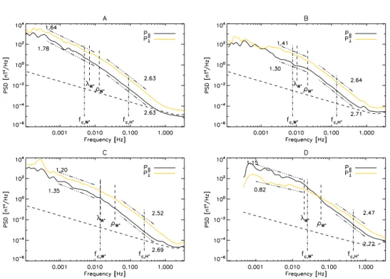
In the first part of this thesis, we analyze the statistical properties of magnetic field fluctuations measured by the Cassini spacecraft in- side Saturn’s magnetosphere. We introduce Saturn’s magnetosphere as a new laboratory for plasma turbulence, where the background magnetic field is strong (5 nT ≤ B ₀ ≤ 75 nT), fluctuations are weak ( h δB/B i = 0.07) and the ion plasma β _i is smaller than one. We conduct a case study of the second orbit of Cassini and find the statistics of the fluctuations on MHD scales to be characterized by large scale non-stationary processes. The spectral index on these scales varies between 0.8 and 1.7. At higher frequencies, we observe a steeper spectrum with nearly constant power-law exponent. A spectral break on ion scales separates the two frequency ranges.

We carry out a statistical study of the high frequency, kinetic range, fluctuations using the first seven orbits of Cassini. To account for the changing plasma conditions in the magnetosphere, we use power spectral densities transformed to wave number space normalized to ion scales. At radial distances greater than 9 R _s , we observe an av- erage slope of 2.6 on kinetic scales, but closer to Saturn the spectral indices tend to get shallower. Within error limits, these results are in accordance with a critically balanced cascade of kinetic Alfvén waves. Probability density functions of the fluctuations have in- creasingly non-Gaussian tails with increasing frequency. The flatness grows with frequency like a power-law indicating intermittency and formation of coherent structures.

We show that the dissipation of magnetic field fluctuations has im-

portant implications for Saturn’s magnetosphere. We estimate the

total energy flux along the turbulent cascade as 140 − 160 GW, which

is ultimately dissipated as heat. For Saturn’s magnetosphere, this

turbulent heating mechanism is introduced for the first time. It pro-

vides energy on the same order of magnitude as needed to explain

the large plasma temperatures measured at Saturn. In an extended

data set of 42 orbits, we further analyze the local time and longitude

asymmetries. We observe significantly stronger fluctuations in the

pre-noon sector of the outer magnetosphere and the midnight sector

close to the planet. The spectral energy and the turbulent heating

rate are enhanced in a longitude range that coincides with regions of

denser plasma.

evaluate one-dimensional reduced power spectral densities from ar- bitrary energy distributions in wave vector space. We assume ax- isymmetry and approximate the poloidal fluctuations to be passively cascaded by Alfvénic fluctuations. The diagonal elements of the spec- tral tensor can be calculated separately and we are able to analyze the implications of the measurement geometry. Based on a critically balanced turbulent cascade, we construct an energy distribution in three dimensional k-space from MHD to electron scales.

We investigate the power spectra in detail and focus on the spectral slope as a function of field-to-flow angle θ and of outer scale. We show for the first time that critically balanced turbulence develops toward a θ-independent cascade with a quasi-perpendicular spectral slope.

This occurs at a frequency f max , which is analytically estimated and is controlled by the outer scale, the critical balance exponent and the field-to-flow angle. We also discuss anisotropic damping terms acting on the k-space distribution of energy and their effects on the PSD. Here, the dominating parameter is the electron temperature, which controls the onset of damping.

We calculate synthetic spectra for given measurement geometries and plasma parameters in the solar wind and compare them to recent observations that are interpreted in terms of a critically balanced turbulent cascade. A qualitatively successful reproduction of the observations indicates that the results are indeed in agreement with a critically balanced cascade of (kinetic) Alfvén waves. However, we find that the addition of a damping term is substantial to obtain a smooth transition of spectral slopes from small to large field-to-flow angles.

In order to corroborate our interpretation of turbulence at Saturn, we

model magnetospheric power spectral densities using data presented

in the first part of this thesis. We qualitatively reproduce the location

of the spectral break and the spectral slopes on MHD and kinetic

scales for a selected spectrum discussed in the case study. Further,

we model the observed radial distribution of spectral indices and

find that damping on scales of the hot electrons might explain the

shallower spectral slopes inside 9 R _s . These results indicate that

the energy transferred along the turbulent cascade is predominantly

deposited into the hot electron population.

Der erste Teil dieser Dissertation befasst sich mit der Analyse sta- tistischer Eigenschaften von Magnetfeldfluktuationen in der Magne- tosphäre des Planeten Saturn. Dabei zeigen wir zum ersten Mal, dass sich auf kinetischen Skalen eine turbulente Kaskade ausbildet, welche innerhalb der mittleren Magnetosphäre einen konsistenten spektralen Index aufweist. Wir stellen damit die Magnetosphäre als ein - zusätzlich zum Sonnenwind - neues Labor für die Turbulenz- analyse vor, welches sich durch ein starkes Hintergrundmagnetfeld (5 nT ≤ B ₀ ≤ 75 nT), schwache Fluktuationen ( h δB/B ₀ i = 0.07) und ein Ionen-Plasma β _i kleiner Eins auszeichnet. Mittels einer Fallstudie des zweiten Orbits von Cassini zeigen wir, dass die statistischen Ei- genschaften von Fluktuationen auf MHD Skalen hauptsächlich durch großskalige magnetopshärische Prozesse bestimmt werden. Der spek- trale Index auf diesen Skalen variiert zwischen 0.8 und 1.7. In einem höheren Frequenzbereich, der durch einen spektralen Bruch auf Io- nenskalen eingeleitet wird, beobachten wir einen steileren Verlauf mit geringerer Variation des spektralen Indexes.

Wir führen eine statistische Studie der spektralen Dichten auf kineti- schen Skalen durch, wofür die ersten sieben Orbits von Cassini ver- wendet werden. Der mittlere spektrale Index beträgt 2.6 und verrin- gert sich innerhalb von 9 R _s zu ∼ 2.3. Innerhalb der Fehlergrenzen lassen sich diese Ergebnisse durch eine turbulente Kaskade von kine- tischen Alfvénwellen im kritischen Gleichgewicht erklären. Im Ver- hältnis zu einer Gaußverteilung sind extreme Fluktuationen häufiger anzutreffen. Dieser Effekt verstärkt sich mit ansteigender Frequenz und die Flatness steigt als Funktion der Frequenz einem Potenzgesetz gleich an. Letzteres ist ein deutliches Zeichen von Intermittenz.

Die Dissipation der magnetischen Fluktuationen hat starke Aus-

wirkung auf die Energiebilanz der Magnetosphäre und der gesam-

te Energiefluss entlang der Kaskade wird auf etwa 140 − 160 GW

abgeschätzt. Unter der Annahme, dass diese Energie in Form von

Wärme dissipiert wird, ließen sich die hohen Plasmatemperaturen in

der Magnetosphäre erklären. Es ist das erste Mal, dass eine solche

turbulente Heizungsrate für das Saturnsystem aufgestellt wird. Mit

einem erweiterten Datensatz von 42 Orbits untersuchen wir weiter-

hin die Abhängigkeit der gewonnenen Parameter von der Lokalzeit

insbesondere im Vormittagssektor der äußeren Magnetosphäre und im Mitternachtssektor auf kurzer Distanz zum Planeten auftreten.

Außerdem stellen wir erhöhte spektrale Dichten und Heizungsraten auf planetaren Längen fest, auf denen ebenfalls eine erhöhte Plasma- dichte beobachtet wurde.

Im zweiten Teil dieser Dissertation stellen wir ein numerisches Mo- dell vor, mit Hilfe dessen sich reduzierte eindimensionale spektrale Dichten aus einer gegebenen Energieverteilung im k-Raum berechnen lassen. Diese hängen ebenfalls von der Messgeometrie und den zu- grunde liegenden Plasmaparametern ab. Unsere Annahmen zur Her- leitung des Modells sind axialsymmetrische Fluktuationen und eine durch toroidale Fluktuationen kontrollierte passive Kaskade von po- loidalen Fluktuationen. Damit können wir die diagonalen Elemente des spektralen Tensors einzeln berechnen und untersuchen ausführ- lich die Eigenschaften einer turbulenten Kaskade von (kinetischen) Alfvénwellen im kritischen Gleichgewicht.

Zum ersten Mal kann gezeigt werden, dass sich der spektrale Index einer solchen Kaskade bei hohen Frequenzen verändert. Die spek- tralen Dichten werden quasi-senkrecht und bei entsprechend hohen Frequenzen letztendlich unabhängig vom Winkel θ zwischen Magnet- feld und Plasmageschwindigkeit. Die Frequenz, bei der dies geschieht, wird analytisch approximiert und wird hauptsächlich durch den Win- kel θ, den Exponenten des kritischen Gleichgewichts und die der Energieeinspeisung zugeordnete Länge bestimmt. Wir untersuchen außerdem den Einfluss von anisotropen Dämpfungstermen auf die spektrale Dichte. Hierbei stellt sich heraus, dass insbesondere die Elektronentemperatur maßgeblich für den Einsatz der Dämpfung ist.

Wir verwenden das Modell um zu überprüfen, ob bestimmte Beob- achtungen im Sonnenwind in Übereinstimmung mit einer turbulenten Kaskade im kritischen Gleichgewicht sind. Mittels unserer neuartigen Modellierungsmethode reproduzieren wir qualitativ den gemessenen spektralen Index als Funktion des Winkels θ auf MHD und kineti- schen Skalen und zeigen damit, dass die Ergebnisse tatsächlich in der verwendeten Form interpretiert werden können. Wir stellen fest, dass der Einfluss der Dämpfung erheblich dazu beiträgt einen langsamen Verlauf der spektralen Anisotropie zu erhalten.

Um unsere im ersten Teil getätigte Interpretation der Magnetfeld-

fluktuationen in Saturn’s Magnetosphäre zu erhärten, modellieren

wir eine spektrale Energiedichte, welche im Rahmen der Fallstudie

besprochen wurde. Die Form des Spektrums - sowohl spektrale Indi-

zes als auch der spektrale Bruch - kann qualitativ erfolgreich unter

Verwendung der im ersten Teil verwendeten Plasmaparameter repro-

Elektronenskalen erklären lässt. Diese Ergebnisse legen den Verdacht

Nahe, dass hauptsächlich die heiße Elektronenpopulation in Saturn’s

Magnetosphäre durch turbulente Fluktuationen geheizt wird.

1 Introduction 1

2 Turbulence Theory 5

2.1 Hydrodynamic Turbulence . . . . 5

2.1.1 Symmetries and Stationarity . . . . 6

2.1.2 Kolmogorov Spectrum of Hydrodynamic Turbulence . . . 8

2.1.3 Intermittency . . . . 10

2.2 Plasma Turbulence . . . . 12

2.2.1 MHD Waves . . . . 14

2.2.2 Weak Isotropic Alfvén Wave Turbulence . . . . 16

2.2.3 Weak Anisotropic Alfvén Wave Turbulence . . . . 18

2.2.4 Critically Balanced Turbulence . . . . 19

2.2.5 Turbulence on Kinetic Scales . . . . 22

2.2.6 Kinetic Alfvén Wave Turbulence . . . . 23

2.2.7 On the Ambiguity of Dimensional Analyses . . . . 25

2.2.8 Estimation of the Background Magnetic Field . . . . 26

2.2.9 Dissipation . . . . 28

2.3 Observations in the Solar Wind . . . . 29

2.3.1 Magnetic Power Spectral Densities . . . . 30

2.3.2 Observations of Intermittent Fluctuations . . . . 31

2.3.3 Spectral Anisotropy . . . . 32

3 Turbulence at Saturn 35 3.1 Planetary Properties of Saturn . . . . 35

3.1.1 Saturn’s Moons . . . . 37

3.1.2 Magnetospheric Structure . . . . 39

3.1.3 Rotation Period . . . . 44

3.2 Plasma Dynamics in Saturn’s Magnetosphere . . . . 48

3.3 Turbulent Magnetic Field Fluctuations . . . . 51

3.3.1 Basic Considerations for Magnetospheric Turbulence . . . 51

3.3.2 Processing of Magnetic Field Data . . . . 54

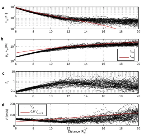
3.3.3 Measured Parameters of the Magnetic Field . . . . 55

3.3.4 On the Geometry of the Observations . . . . 59

3.3.5 Case Study of Cassini’s Second Orbit . . . . 60

3.4 Statistical Analysis of Kinetic Range Turbulent Cascade . . . . . 70

3.4.1 Spectral Index within the Kinetic Range . . . . 72

3.4.2 Intermittency of Fluctuations . . . . 77

3.4.3 Correlation of Spectral Indices with Field-to-Flow Angle . 78 3.4.4 Compressibility Level . . . . 79

3.4.5 Turbulent Plasma Heating Rates . . . . 80

3.5 Asymmetries of Magnetospheric Turbulence . . . . 83

3.5.1 Extended Data Set . . . . 84

3.5.2 Root Mean Square of Fluctuations . . . . 86

3.5.3 Relative Spectral Power on Kinetic Scales . . . . 89

3.5.4 Spectral Index . . . . 91

3.5.5 Turbulent Heating Rates . . . . 93

3.5.6 Discussion and Comparison with Recent Observations . . 99

3.6 Conclusion . . . 102

4 Modeling Turbulent Spectra 105 4.1 General Form of the Spectral Tensor . . . 106

4.1.1 Rotational Symmetry Along Mean Magnetic Field . . . . 107

4.1.2 Fourier Transform of the Correlation Tensor . . . 107

4.1.3 Diagonal Elements of the Spectral Tensor . . . 109

4.2 Numerical Results of Critical Balance Model . . . 111

4.2.1 Power Spectral Density in Frequency Space . . . 112

4.2.2 Transition from MHD to Kinetic Scales . . . 113

4.2.3 Anisotropic Damping . . . 122

4.3 Application to Solar Wind Observations . . . 125

4.3.1 MHD Turbulence . . . 125

4.3.2 Kinetic Range Turbulence . . . 127

4.4 Modeling Spectral Densities at Saturn . . . 129

4.4.2 Reproduction of Distribution of Spectral Indices . . . 135 4.5 Conclusion . . . 137

5 Summary 141

A Cassini: Mission and Instruments 147

A.1 Helium Magnetometer . . . 147

A.2 Fluxgate Magnetometer . . . 150

B Probability Density Functions of Measured Parameters 153

C Numerical Evaluation of Power Spectral Density 157

Introduction

Turbulence is an apparently chaotic flow of fluids that transfers energy from large to small scales. It stems from the Latin word for rotate, perturb, or entangle, all of which illustrate the flow patterns in a turbulent flow. Everyone has already seen or experienced the characteristic turbulent whirls or eddies, e.g., in water behind a bridge head, during a horrible transatlantic flight or - to cite the turbulence scientists’ most popular example - when you pour milk in your coffee. Because of such common presence in our daily lives, it is surprising that a renowned physicist such as Richard Feynman (1918-1988) called turbulence a central unsolved problem of physics (Feynman et al., 2010, Ch. 3). The problem that he is referring to is the inability to exactly describe the particle motions of the fluid when it behaves turbulent, even though we know the underlying equation of motion, namely the Navier-Stokes equation for hydrodynamic flow.

What we can do, however, is describe the motion of the fluid in a statistical sense. If we observe fully developed turbulence on the right scales, i.e., in the inertial range, we find that the averaged velocity fluctuation of the particles is constant in time and independent of location. More importantly, the statistical moments at different scales are related to each other in a way that is universal for all hydrodynamic fluids, regardless of how the energy is injected into the system on large scales. This important result was discovered by A. N. Kolmogorov (1907-1987) and is in detail explained in the book Turbulence by Frisch. This universal scale invariance of the statistical moments stems from the self-similar decay of large eddies to smaller ones. Nonlinear interactions between eddies of comparable size transfer energy along a so-called turbulent cascade from large to small scales. In this thesis, it is this turbulent cascade and the energy transfer along it that we are most interested in.

With the beginning of the space era and the ability to conduct in-situ mea- surements in the solar wind, it became clear that not only fluids on Earth are turbulent, but also the plasmas commonly found in space. Similar to velocity fluctuations in hydrodynamic turbulence, power spectral densities of magnetic fluctuations in the solar wind were found to scale with a power-law of slope 5/3.

However, there are important differences in the governing equations describ-

quasi-neutral ions and electrons is subject to far reaching electromagnetic forces, which leads to a complex collective behavior and the emergence of wave modes that change the energy transfer substantially. It also has characteristic ion and electron scales. On scales much larger than ion scales, the plasma can be de- scribed as a fluid in the framework of magnetohydrodynamics (MHD). However, on smaller scales, so-called kinetic scales, the characteristics of the turbulent cascade change considerably. Lastly, plasma turbulence is inherently anisotropic with regards to a background magnetic field. One approach to explain the ob- served Kolmogorov-like scaling in the presence of anisotropic plasma waves is the concept of a critically balanced turbulent cascade, which we follow in this thesis. It describes the nonlinear interactions of Alfvén waves and their kinetic counterparts, the kinetic Alfvén waves, as most important for the turbulent cas- cade of energy. The relevant turbulence theories - starting from hydrodynamic turbulence - are presented in Chapter 2.

The best laboratory we have for plasma turbulence so far is the solar wind.

Here, the Reynolds number, which quantifies the turbulent flow of a fluid, is orders of magnitudes larger than that of any artificially produced plasma. Solar wind turbulence has been analyzed since more than 30 years and several charac- teristic features have been found that seem to be universal for plasma turbulence.

Here, magnetic field fluctuations have been analyzed most extensively, because they can be determined with high time resolution and accuracy compared to the measurement of other plasma parameters such as the electric field or the plasma velocity. For the same reason, we restrict our analysis to magnetic fluctuations in this thesis. Characteristic features of turbulence in the solar wind include a Kolmogorov-like spectral index of 5/3 on MHD scales and a spectral break around ion scales followed by a steeper slope on kinetic scales. It is believed that turbulent interactions are important to explain the acceleration of ener- getic particles the solar wind and that the dissipation of turbulent fluctuations substantially heats the plasma. Turbulence is therefore essential to describe the dynamical evolution of the solar wind.

As turbulence is an ubiquitous phenomenon, it is interesting to ask where else, besides in the solar wind, we may encounter turbulent fluctuations. Can planetary magnetospheres be turbulent, as Saur et al. (2002) suggest for the case of Jupiter? Is magnetospheric plasma heated by turbulent interactions?

And how would that affect the planetary energy budget? In order to answer

these questions, we conduct for the first time a turbulence analysis for Saturn’s

magnetosphere. In contrast to the effectively infinite size of the heliosphere,

this planetary system is bounded by the magnetopause and the magnetic field

geometry. It is also characterized by a strong planetary magnetic field. Alfvén

waves that are launched inside the magnetosphere through large scale instabil-

ities travel along planetary magnetic field lines and are reflected at the density

gradients close to the planet. Hence, we may conjecture the magnetosphere as

a bath of plasma waves that interact nonlinearly and form a turbulent cascade.

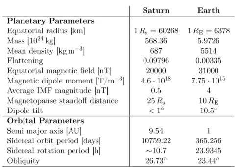
which orbits around Saturn since 2004. Therefore, we have a vast data set pub- licly available through the Planetary Data System ¹ . Despite of this large data set, there are several unanswered questions. One of these questions regards the puzzling high plasma temperatures in the magnetosphere. Although the plasma is produced close to Saturn by the moon Enceladus and expands nearly adiabat- ically as it is transported radially outward, it does not cool down accordingly.

In contrast, the temperature is found to increase with distance to Saturn. This temperature profile can only be explained by a local heating mechanism (Bagenal and Delamere, 2011). In this thesis, we elaborate on the idea that the dissipation of turbulent magnetic fluctuations provides the energy that is required to heat the plasma to the observed temperatures.

In Chapter 3, we conduct a spectral analysis of magnetic field data obtained in Saturn’s magnetosphere, part of which has already been published in von Pa- pen et al. (2014). In Section 3.1, we introduce the second largest magnetosphere of the solar system, which is primarily internally controlled, i.e., the magneto- spheric dynamics are mostly fueled by internal sources and by the rapid rotation of the planet. The analysis in the framework of turbulence is thus complicated by large scale plasma processes in Saturn’s magnetosphere. After we present the most relevant plasma dynamics of Saturn’s magnetosphere in Section 3.2, we analyze in detail the magnetic field data and the power spectral densities in a case study in Section 3.3. We observe a turbulent cascade that is constantly present on kinetic scales and conduct a statistical study in Section 3.4. Here, we estimate the energy that is transferred along the cascade and is ultimately dissipated as heat. The results indicate that turbulent heating is indeed substan- tial for the magnetospheric energy budget and might help to explain the high plasma temperatures. In Section 3.5, we further analyze the spatial asymmetries in Saturn’s magnetosphere with regards to local time and planetary longitude.

We show that the turbulent heating rate correlates with planetary longitude and maximizes at longitudes where a higher plasma density is detected.

The results in Saturn’s magnetosphere can be interpreted in terms of a crit- ically balanced turbulent cascade formed by kinetic Alfvén waves. This theory of strong turbulence has been proposed to explain the observations in the inter- stellar medium and the solar wind in the presence of anisotropy (Goldreich and Sridhar, 1995). It is based on the conjecture of a critical balance between wave period and nonlinear time and can be defined by the energy distribution in wave vector space. For this theory, power spectra can be calculated analytically only for the extreme cases of a background magnetic field parallel or perpendicular with respect to the plasma flow. However, the field-to-flow angles during in-situ measurements are generally variable and the magnetic field is therefore never perfectly parallel or perpendicular to the flow. Still, it is currently unknown how exactly power spectra scale for such intermediate field-to-flow angles. For

1

http://ppi.pds.nasa.gov

in frequency space from a given energy distribution in three-dimensional wave vector space for arbitrary measurement geometries. With this method, we can construct for the first time power spectral densities of critically balanced turbu- lence from MHD to electron scales.

We present this method and the associated analysis in Chapter 4. After

we introduce the theoretical framework for this tool in Section 4.1, we test the

synthetic models in detail. Interestingly, we find in Section 4.2 that certain

assumptions that are implicitly made in the literature, e.g., the constancy of

the spectral index with frequency, are not in agreement with a critically bal-

anced cascade. We also show that damping effects are more important than

previously thought, which has important consequences for the interpretation of

turbulent fluctuations. As the tool proves to be useful for the interpretation

of recent solar wind observations in Section 4.3, we also apply it to our results

in Saturn’s magnetosphere in Section 4.4. This forward modeling method cor-

roborates our former interpretation in terms of critically balanced turbulence in

Saturn’s magnetosphere and indicates that the energy of the turbulent magnetic

field interactions is primarily deposited into the hot electron population at Sat-

urn. In the final Chapter 5, we summarize the results of the analyses and draw

our conclusions.

Turbulence Theory

In this chapter, we introduce the main concept of this thesis, namely the energy transfer controlled by nonlinear interactions that form a turbulent cascade. We begin with the description of hydrodynamic (HD) turbulence in Section 2.1 using a dimensional analysis. This analysis leads to a universal scaling law for velocity fluctuations. Then we proceed to plasma turbulence in Section 2.2, in which we introduce magnetohydrodynamics (MHD) and present the most important MHD wave modes. We show that a dimensional analysis for MHD results in non- universal scalings and discuss several MHD turbulence theories, where we focus on critically balanced turbulence after Goldreich and Sridhar (1995). On scales smaller than typical MHD scales, kinetic effects change the turbulent cascade and different wave modes emerge. The critically balanced cascade is extended into the kinetic range and we shortly debate the ambiguity of dimensional analysis.

Further, we discuss the dissipation range of the turbulent cascade and potential damping mechanisms. The applicability of the introduced turbulence theories is described at the end of this chapter in Section 2.3. Here, we present the solar wind observations that are most relevant for our further analysis of magnetic field fluctuations in Saturn’s magnetosphere.

2.1 Hydrodynamic Turbulence

Turbulence is an ubiquitous phenomenon, which is observed in all kinds of fluids.

It is characterized by an apparent chaotic flow on a wide range of scales. Obser-

vations of turbulent flow patterns date back to Leonardo da Vinci (1452-1519),

who not only drew the turbulent flow of water with characteristic eddies, but also

described the self-similarity of the vortices (see e.g. Frisch, 1995). Around three

hundred years later, the now-called Navier-Stokes equation of motion was de-

rived, which allows for a mathematical description of the phenomenon. Indeed,

∂ _t v + (v · ∇ )v = − 1

̺ ∇ p + ν ∆v + f (2.1)

∇ · v = 0 (2.2)

probably describe everything we need to know about incompressible turbulence as long as we are not interested in quantum scales (Frisch, 1995). Theoretically, the problem is solved: We could insert the complete set of parameters for the fluid elements as there are velocity v, density ̺, pressure p, kinematic viscosity ν, and external force density f that may act on the fluid at an instant t ₀ and calculate their dynamical evolution. Practically, however, this is impossible.

Therefore, a statistical approach seems more promising to describe the mean properties of an ensemble of particles.

To quantify the turbulence of a flow, one can estimate the ratio of the non- linear term to the dissipation or viscous term in Equation (2.1), which is called the Reynolds number:

Re ∼ (v · ∇ )v ν∆v ∼ vL

ν . (2.3)

Here, we used a dimensional analysis to derive the last term. In this context and throughout this thesis, ’ ∼ ’ means ’on the same order of magnitude’. The parameter L comes from the gradient of the velocity and is a characteristic length of the system, on which a significant change in velocity is observed. It is usually interpreted as the scale on which energy is injected into the system.

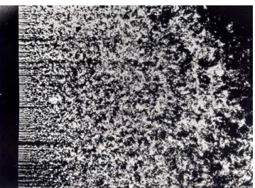
In the case of a fluid flowing past an obstacle, this so-called outer scale may be the diameter of the obstacle. For Re ≪ 1, we speak of a laminar flow, i.e., there is no turbulent mixing and neighboring stream lines stay next to each other at all times. At slightly higher Reynolds numbers Re ∼ 10, the flow begins to develop stationary eddies behind the obstacle and at even higher numbers, Re ∼ 100, the so-called Kármán vortex street emerges (Frisch, 1995). The Reynolds number that marks the transition from laminar to turbulent flow is called the critical Reynolds number, Re _crit . For Reynolds numbers Re ≫ Re _crit the flow will evolve to fully developed turbulence, a term coined by Sir William Thomson, Lord Kelvin (Thomson, 1887). Figure 2.1 shows an example of such a hydrodynamic turbulent flow behind a grid.

2.1.1 Symmetries and Stationarity

From Figure 2.1 it is fairly clear that the motion of a single fluid particle behind

the grid is chaotic and asymmetric and also differs at every location. However,

if we look at the mean velocity fluctuations h v(r, t) i , averaged over a sufficiently

large region around location r or over a sufficiently large time interval around

time t, we will find that the mean velocity of such a group of particles is in-

dependent of the location as long as it is far away from the grid and from the

Figure 2.1: Example of an homogeneous isotropic turbulent flow behind a grid (with permission of H. Nagib, FDRC-IIT).

system’s boundaries. Hence, in a statistical sense, the flow’s velocity fluctuations are homogeneous in fully developed turbulence.

As long as we have a non-vanishing mean flow, V = h v(r, t) i , the flow has a preferred direction and the turbulence seems anisotropic. However, to describe the statistics of a fluid in the framework of turbulence, it is best to look at the fluctuations in the rest frame of the fluid. This perspective can be easily achieved as the governing Navier-Stokes Equation is invariant under Galileo transformations, (r ^′ , v ^′ ) → (r+V · t, v+V). We can thus subtract any mean flow V and only consider the centered variable, v(r, t) = v ^′ (r, t) − V, which we call the fluctuation. Now, there is no preferred direction anymore and it can be shown that the fluctuations are in fact statistically isotropic. Therefore, it suffices to use a scalar value v(r, t) as random variable to describe the statistics without loss of information. If the rate of energy injected into the system is constant or, in the case of grid turbulence, if the incident fluid flow is constant, we can expect the turbulent motions behind the grid to be quasi-stationary in a statistical sense. This means that the statistical properties are also invariant under time translation and thus are constant in time. In a stationary, homogeneous and isotropic flow, we may therefore measure the velocity fluctuation v(r, t) at any location, time and in any direction without effect on the resulting statistics.

According to Frisch (1995), we may write this as

v(r, t) ^law = v(r + r ^′ , t + t ^′ ) , (2.4) which he calls equality in law. This means that the statistical properties of the variables on both sides of Equation (2.4) are the same.

However, in real measurements we usually obtain finite time series and, thus,

we can only estimate the fluctuations’ statistical moments. The shorter the time

series, the larger is the error of such an estimation. The real statistics of a

PDF defines the probability to measure a certain velocity v and contains all information on the statistical moments

h v ⁿ i = Z

dv v ⁿ p(v) (2.5)

of order n. The ergodicity theorem now states that the estimated time average of the fluctuating quantity v will be equal to the real ensemble average over the PDF if the time interval T is sufficiently large (Frisch, 1995)

h v ⁿ i = Z

dv v ⁿ p(v) ≈ 1 T

Z T

0

v ⁿ dt . (2.6)

This result is an important basis for our further analysis. It shows that we can make assumptions about the statistics of the system under consideration based on finite time measurements. These measurements can be conducted at any time and location if the turbulence is fully developed, homogeneous, and stationary. It can be shown that the time interval T needed to correctly estimate the statistical moments h v ⁿ i , grows rapidly with order n (Frisch, 1995). The same holds for the corresponding sample size N = T /∆t for a given time resolution ∆t. This means that we need very long time series to resolve the tails of the PDF, which describe rare extreme events. We therefore restrict our later estimations to the normalized fourth order statistical moment, which is the flatness.

2.1.2 Kolmogorov Spectrum of Hydrodynamic Turbulence In 1941, A. N. Kolmogorov published four papers on hydrodynamic turbulence, which can be seen as the beginning of modern turbulence research (Kolmogorov , 1941a,b,c,d). A major contribution of his work was the derivation of the famous four-fifths law (Kolmogorov, 1941c), which is a mathematically exact result and describes the dissipation of energy. However, we restrict ourselves to a phe- nomenological derivation. For a detailed review of Kolmogorov’s theory, we refer the reader to the book Turbulence by Frisch.

If energy is injected into a system on a length scale L, eddies of diameter d ∼ L will be generated, which have a typical velocity fluctuation v _L . Here, v _L ∼ p h δv ² i is the root-mean-square (RMS) of the velocity fluctuations’ increment,

δv(r, L) = v(r + L) − v(r) , (2.7) and can be thought of as the average velocity difference on the corresponding scale L. The eddies will nonlinearly interact with each other and decay to form smaller eddies on a scale ℓ < L with mean velocity difference v _ℓ on scale ℓ.

The time, in which an eddy of size ℓ is significantly distorted, is denoted by the

Figure 2.2: Richardson cascade of hydrodynamic turbulence (Frisch, 1995).

characteristic nonlinear time

τ _nl ∼ ℓ

v _ℓ . (2.8)

It is also called eddy-turnover time. The smaller eddies may fill the whole system space, so that despite of less kinetic energy per eddy, v ² _ℓ , the total energy flux is conserved. This decay will go on to smaller scales until a dissipation scale η _d is reached, where the fluctuations’ energy is converted into heat. This evolution is pictured in the so-called Richardson cascade, which is schematically shown in Figure 2.2. Here, we separate the cascade into three regions: (1) the energy injection range on scales ℓ ∼ L, (2) the inertial range on scales ℓ, where L ≫ ℓ ≫ η _d , and (3) the dissipation range on scales ℓ ∼ η _d . In hydrodynamic turbulence, the inertial and dissipation ranges, where the energy is nonlinearly transported from large to small scales and finally dissipated as heat, behave in a universal way independent of the type of fluid.

In a stationary turbulent cascade, the energy injection rate is equal to the dissipation rate. As a result, the kinetic energy E ∼ v ² _L of the largest eddies on scale L per unit time is also equal to the energy flux through scale ℓ

E ˙ ∼ v ² _ℓ

τ _tr ∼ ǫ , (2.9)

where ǫ denotes the dissipation rate. In the inertial range, the energy is trans- ferred to smaller scales within a characteristic transfer time τ _tr = τ _tr (ℓ), which is a function of scale ℓ. In hydrodynamics, the transfer time is equal to the non- linear or eddy-turnover time τ _tr ∼ τ _nl . Inserting this relation in Equation (2.9) leads to

ǫ ∼ v ³ _ℓ

ℓ ⇔ v _ℓ ∼ (ǫℓ) ^1/3 , (2.10)

E _k = E _k (k) as a function of wave number k ∼ ℓ ⁻¹ . The energy spectrum is related to the total energy by v _ℓ ² ∼ E _k k and can be written as

E _k ∼ v _ℓ ² k ⁻¹ ∼ ǫ ^2/3 k ^−5/3 . (2.11) Equation (2.11) determines the Kolmogorov spectrum and shows that the power spectra P (k) in the inertial range follow a power-law k ^−κ with spectral index κ = 5/3. This is experimentally verified for various fluids (e.g. Gibson and Schwarz , 1963). The inertial range reaches to the so-called Kolmogorov dissipation scale

η _d ∼ ν ³

ǫ 1/4

. (2.12)

Here, dissipation caused by particle collisions sets in and ultimately leads to heating of the fluid (Kolmogorov , 1941a; Frisch, 1995). It is interesting to note, that the dissipation scale does not depend on the energy injection mechanism.

2.1.3 Intermittency

The Richardson cascade as shown in Figure 2.2, consists of eddies that decay to smaller self-similar eddies, which fill the whole space. This is also a crucial point in the hypotheses leading to the derivation of Kolmogorov’s four-fifths law (Frisch, 1995, Ch. 6). Space filling eddies lead to a turbulent signal that shows consistent statistical properties at all times and at all scales according to

δv(r, λℓ) ^law = λ ^h δv(r, ℓ) . (2.13) Therefore, the statistics are scale invariant under an associated transformation.

Kolmogorov suggested that the scaling exponent h = 1/3 is unique and universal for all kinds of fluids. However, Batchelor and Townsend (1949) discovered that the signal at wave numbers close to the dissipation scale gets increasingly bursty.

These extreme events happen only at a fraction of the time while the flow seemed inactive during the rest of the time. Such a behavior violates Equation (2.13) and a function displaying this characteristic is said to be intermittent (Frisch, 1995; Wan et al., 2012).

To measure the intermittency, one often uses so-called structure functions,

S _n (ℓ) ≡ h (v(r + ℓ) − v(r)) ⁿ i = h δv(r, ℓ) ⁿ i , (2.14)

which can be estimated with the help of increments. The variable n defines the

order of the structure function. In the following, we drop the dependence on

location r assuming that the average is taken over a large enough area or time

to assume homogeneity. The structure functions are known to follow power-

laws in the inertial range, S _n (τ ) ∝ τ ^ξ(n) , where ξ(n) is called scaling exponent

(Frisch, 1995). For self-similar fluctuations, the scaling exponent varies with

−5 −4 −3 −2 −10 0 1 2 3 4 5 0.2

0.4 0.6 0.8 1

x/σ

p(x)/p(0)

−5 −4 −3 −2 −1 0 1 2 3 4 5 10⁻³

10⁻² 10⁻¹ 10⁰

x/σ

p(x)/p(0)

F=3 F=4

Figure 2.3: Probability density function p(x) of a normal distributed centered variable x (Gaussian, black line) with flatness F = 3 and near- Gaussian PDF with increased tails and flatness F = 4 (red line). Both PDF are normed at x = 0 and normalized by their standard deviation σ.

The left panel shows a linear plot while the right panel shows the same plot with logarithmic y-axis. Here, the increased tails are much clearer.

order n as ξ(n) = h · n, where h is the Hurst exponent (e.g. Carbone et al., 1995;

Kiyani et al., 2009; Salem et al., 2009; Mangeney , 2012). Deviation from this simple linear law is generally called multifractality. Indeed, a straight forward application of Equation (2.13) with h = 1/3 to the structure functions yields S n (ℓ) ∝ ℓ ^n/3 . Yet, measurements have shown that the scaling exponent of the structure functions is not linear in n but rather a nonlinear function ξ _n (see e.g.

Burlaga, 1992; Sorriso-Valvo et al., 2001; Kiyani et al., 2009; Salem et al., 2009, for measurements in the solar wind). We may therefore write

S _n (ℓ) ∝ ℓ ^ξ

. (2.15)

Physically, this may be understood as a correction to the Richardson cascade.

Wind tunnel measurements conducted by Argoul et al. (1989) indicate that a large scale eddy may decay asymmetrically into two smaller eddies of different energies. If this asymmetric decay is repeated across all scales, energetic fluctua- tions will concentrate in certain locations forming intermittent or bursty signals.

This process might further be scale dependent, which is then equivalent to a multifractal formalism (Meneveau and Sreenivasan , 1991; Burlaga, 1992; Muzy et al., 1993; Kiyani et al., 2013).

At this point it is instructive to envision the probability density function p(δv) of the random variable δv as it is shown in Figure 2.3. If the random variable is normal and centered, its PDF will be a Gaussian as shown by the black line. On the other hand, if extreme events are more likely to happen, which is the case for intermittent signals, the so-called tails of the probability density function will be increased. This is shown by the red line in Figure 2.3.

This feature is much easier to detect when the y-axis is scaled logarithmically

as shown in the right panel. The increase of the tails can be quantified by the

F = δv ⁴

h δv ² i , (2.16)

which is a function of scale ℓ. A normal distribution yields a flatness of F = 3. A larger flatness, F > 3, means that the tails are enhanced and therefore extreme events are observed more often. The flatness can also be expressed in terms of structure functions

F(ℓ) = S ₄

S ² ₂ ∝ ℓ ^ξ

^−2ξ

. (2.17) This shows that the flatness for strictly self-similar decay is constant at all scales, because the exponent vanishes for a function ξ n that is linear in n. The flat- ness can thus be used to estimate if the scaling exponent is nonlinear. Indeed, turbulence measurements in the solar wind and planetary magnetospheres have shown that the flatness of magnetic field fluctuations increases as a power-law for decreasing scales, which is in accordance with intermittent fluctuations (Bruno et al., 2003; Vörös et al., 2002; Alexandrova et al., 2008a) and implies the forma- tion of coherent structures (Mangeney , 2012). This method has the advantage of measuring only moments of fourth order instead of several higher order structure functions, which would be needed to verify the nonlinearity of ξ(n). However, in order to reliably measure the higher order structure functions, one needs an increasing amount of data. This means, that if we estimate the intermittency with the scale dependent flatness F (ℓ), we can use shorter time intervals for our analysis.

2.2 Plasma Turbulence

So far, we have described the principles of hydrodynamic turbulence, where the energy is transferred to smaller scales by interaction of structures such as eddies.

But what happens if we consider a plasma? Plasma is a quasi-neutral ensemble of ions and electrons and therefore it is subject to electromagnetic forces

F = q _s (E + v s × B) , (2.18)

where q _s is the charge of particle s, E the electric field, v _s the mean velocity of particle s and B the magnetic field. If we add this force to Equation (2.1), we will get two equations of motion: one for ions with number density n i and one for electrons with number density n _e . Adding the two equations for an inviscid plasma (ν = 0) and using quasi-neutrality, n _i ≈ n _e , we can derive the magnetohydrodynamic (MHD) equation of motion

̺ (∂ _t v + (v · ∇ )v) = −∇ p + j × B . (2.19)

In MHD, the plasma is treated as a fluid. This treatment is valid for scales much larger than the ion gyro radius

ρ _i =

p 2m _i k _B T _i,⊥

eB ₀ (2.20)

with ion mass m _i , Boltzmann constant k _B , perpendicular ion temperature T _i,⊥ , elementary charge e and background magnetic field B ₀ . The frequencies under consideration in MHD must be much lower than the ion cyclotron frequency

Ω _ic = eB ₀

m _i , (2.21)

Using Ampére’s law, where displacement currents can be neglected because of the low-frequency approximation, the Lorenz force term can be written as

j × B = −∇ p _B + 1

µ ₀ (B · ∇ )B . (2.22)

Here, p _B = B ² /(2µ ₀ ) describes the magnetic pressure and the second term on the right hand side of Equation (2.22) describes the magnetic convection. For a complete description of the fluid motion of the plasma on MHD scales, we further need the induction equation

∂ _t B = −∇ × E (2.23)

and the generalized Ohm’s law

E + v × B = ηj , (2.24)

where η = (µσ) ⁻¹ is the magnetic diffusivity that depends on the magnetic per- meability µ and the electric conductivity σ of the plasma. For the derivation of Equation (2.24), we have further dropped the terms describing anisotropic elec- tron pressure, electron inertia and the Hall term (Baumjohann and Treumann, 1997, Eq. 7.53). For the plasmas considered in this thesis, the conductivities are very high, so that we may simplify Equation (2.24) to E = − v × B. This means that the plasma is frozen-in to the magnetic field lines and if we insert this relation into Equation (2.23), we will see that

∂ _t B = ∇ × (v × B) . (2.25)

If the frozen-in theorem applies, we may identify velocity and magnetic field fluctuations: δv ∼ δb.

With the help of Elsässer’s variables z ^± = v ± B/(µ ₀ ̺), one can simplify

Equations (2.19) and (2.25) into a form similar to the Navier-Stokes equation

(Elsässer , 1950). While any mean velocity V can be subtracted with Galileo

transformations, this is not possible for a mean magnetic field B ₀ = h B i . There-

with the Alfvén velocity V _A = B ₀ /(µ ₀ ̺) and the fluctuation field h δz ^± i = 0.

Consequently, Equations (2.19) and (2.25) can be written together as

∂ _t ± V _A ∂ _k

δz ^± + δz ^∓ ∇ δz ^± = − ̺ ⁻¹ ∇ p _T , (2.26) where the differentiation ∂ _k is parallel to the background magnetic field B ₀ , p T = p + p B is the total pressure and we used both ∇ · v = 0 and ∇ · B = 0.

It is illustrative to write the MHD equations with Elsässer’s variables because it reduces the MHD equations to a set of equations that look almost identical to the Navier-Stokes equation. This implies that we may use a similar dimen- sional derivation for plasma turbulence to the one we applied for hydrodynamic turbulence.

2.2.1 MHD Waves

One important difference between HD and MHD turbulence is the influence of waves on the turbulent cascade, which can be neglected for hydrodynamic tur- bulence. Although HD waves play an important role in weak or wave turbulence (see, e.g., Nazarenko , 2011), they are only a minor contributor to the strong HD turbulence described in Section 2.1.2. This is because the energy in strong HD turbulence is cascaded by eddies and not weakly interacting waves. However, waves play an important role for the turbulent cascade in plasmas. We will show in this section, what kind of waves are obtained from the MHD equations, i.e., Equations (2.19) and (2.23), and discuss their importance for the cascading process. For a detailed derivation of the MHD dispersion relation the reader is referred to Baumjohann and Treumann (1997, Ch. 9.4).

Alfvén Waves

The linearized MHD equations combined with the continuity equation and the assumption of adiabatic pressure fluctuations can be solved by transverse Alfvén waves, whose dispersion relation is given by

ω = ± k _k V _A . (2.27)

The group velocity of Alfvén waves is the Alfvén velocity V _A , which is strictly parallel or antiparallel to the magnetic field and describes the propagation of a wave packet. The wave fronts, on the other hand, travel in oblique angles to the magnetic field with phase velocity

v _ph,A = ω/k = V _A cos θ _kB . (2.28)

Here, θ _kB is the angle between wave vector k and background magnetic field B ₀ .

The Alfvén wave is a purely transverse wave and most of the plasma fluctuations

in the solar wind on MHD scales are observed to be of Alfvénic nature (Belcher

and Davis , 1971; Matthaeus and Goldstein, 1982; Tu et al., 1984). The nonlin- early interacting fluctuations of Alfvén waves are thus the main contributor to the turbulent cascade.

Note, that Equation (2.27) can also be obtained from the linearized Equa- tion (2.26), resulting in Alfvén waves δz ⁺ and δz ⁻ traveling along and antipar- allel to the background magnetic field B ₀ , respectively (see also Sridhar , 2011).

Here, the structure of the nonlinear term, δz ^∓ ∇ δz ^± , shows an inherent property of Alfvénic turbulence: if there are only Alfvén waves propagating in one direc- tion, e.g., δz ⁺ 6 = 0 and δz ⁻ = 0, the nonlinear term will vanish. This means, that only Alfvén waves propagating in opposite direction can nonlinearly interact with each other.

Compressible Modes

In the compressible case, two additional MHD waves arise, the fast and slow mode. The fast mode, where velocity and density fluctuations are positively correlated, is supposed to be decoupled from the turbulent cascade (Lithwick and Goldreich , 2001; Cho and Lazarian, 2005). Measurements in the solar wind suggest that fast modes are only a minor constituent of the fluctuations (Howes et al., 2012; Klein et al., 2012; TenBarge et al., 2012). Further, fast modes are expected to be strongly damped in high β plasmas, where β = p/p B is the ratio of plasma to magnetic pressure, and dissipated after they steepen into shocks (Schekochihin et al., 2009).

The slow mode seems to be more interesting for the turbulent cascade. It is estimated that around 10% of the fluctuations in the solar wind are caused by the pressure-balanced slow mode, i.e., the compressible component in the solar wind is almost entirely generated by the slow mode (Howes et al., 2012;

Klein et al., 2012; TenBarge et al., 2012). The slow modes are also decoupled from the Alfvénic cascade, but their damping rate is proportional to k _k , which - for wave vectors k _⊥ ≫ k _k - is slow enough to allow for passive mixing by Alfvénic fluctuations (Howes et al., 2006). Here, k _⊥ and k _k are the wave vectors perpendicular and parallel to the background magnetic field B ₀ . Therefore, although they do not develop a cascade on their own, compressible fluctuations are assumed to have a similar scaling as the purely transverse Alfvénic turbulent cascade (Lithwick and Goldreich , 2001; Schekochihin et al., 2009). However, recent observations show that this is not entirely true (Forman et al., 2011;

Wicks et al., 2012).

Non-linear Alfvén Wave Collisions

As can be seen from Equation (2.26), only counter-propagating Alfvén waves

interact which each other. In a purely linear framework, which we adapted for

the derivation of the MHD waves, wave fronts do not interact at all. They may

interfere positively or negatively, but there is no energy transfer between the

waves. Wave-wave interactions are therefore nonlinear interactions and these

scales. Despite of the importance for the turbulent cascade, it is not well known what actually happens during a nonlinear collision of wave fronts.

Howes and Nielson (2013) analyzed the collision of Alfvén waves in weak turbulence and could show that two counter propagating primary waves with the same frequency ω ₁ and wave vectors k ⁺ ₁ and k ⁻ ₁ first undergo a non resonant three wave interaction satisfying

k ⁺ ₁ + k ⁻ ₁ = k ₂ and ω ₁ + ω ₁ = ω ₂ , (2.29) thus forming a secondary wave with wave vector k ₂ and frequency ω ₂ . As the dis- persion relation for Alfvén waves is ω = | k _k | v _A and as only counter-propagating waves can interact, the Equations (2.29) necessarily lead to k _k2 = 0. This means that the secondary wave is not an Alfvén wave but a purely nonlinear wave.

Figure 2.4 shows schematically, where the involved waves are located in wave vector space. The two primary counter-propagating waves with wave vectors k ₁ ^± , denoted by the red circles, interact nonlinearly to form the secondary wave with wave vector k ₂ (green triangle). After Howes and Nielson (2013), this in- trinsically nonlinear secondary wave further interacts with each primary wave, which effectively transfers energy to tertiary waves with frequency ω 3 = ω 1 and wave vectors k ^± ₃ (blue squares). During these interactions energy is cascaded in perpendicular direction only, i.e., the tertiary waves have the same parallel wave number as the primary waves k ^± _k1 = k _k3 ^± . This result has been numerically vali- dated in Nielson et al. (2013) and indicates that the turbulent cascading process is predominantly perpendicular to the background magnetic field.

2.2.2 Weak Isotropic Alfvén Wave Turbulence

The idea that Alfvén waves take the role of the nonlinearly interacting eddies in plasma turbulence led Iroshnikov (1964) and Kraichnan (1965) (IK) to the derivation of a phenomenological spectrum based on the linear wave period of Alfvén waves. Due to the weak interaction of these linear waves, the theory describes weak or wave turbulence. They defined a new interaction time, the Alfvén time

τ _A ∼ (kV _A ) ⁻¹ . (2.30)

The fluctuations are expressed as magnetic fluctuations δb and the plasma is frozen-in to the magnetic field. The emergence of another characteristic time necessarily leads to ambiguity in the phenomenological derivation, which we discuss in more detail in Section 2.2.7. It is important to note here, that despite of the presence of a background magnetic field B ₀ Iroshnikov and Kraichnan assumed isotropic interactions - a fact for which this theory is often criticized (Montgomery and Turner , 1981; Sridhar and Goldreich , 1994).

The Alfvén time can be interpreted as the duration of the interaction of two

Alfvén waves of comparable wave length ℓ ∼ k ⁻¹ , which is much smaller than the

nonlinear time τ _A ≪ τ _nl . This means that during an interaction of two Alfvén

Figure 2.4: Nonlinear interactions during a collision of two primary Alfvén waves with wave vectors k ^± ₁ (red circles) in a plane perpendicular to the background magnetic field. The parallel wave number is given in gray.

The two counter-propagating primary waves interact to form a purely non- linear secondary wave with wave vector k ₂ (green triangle). This secondary wave then interacts with the primary waves to form the tertiary waves with wave vectors k ₃ ^± (blue squares). Figure from (Howes and Nielson, 2013)

wave packets only a small amount of energy can be exchanged:

δE ∼ δb ² τ _A

τ _nl . (2.31)

Therefore, multiple interactions are needed to exchange energy of order unity.

These interactions are randomly phased, so that N ∼ τ _nl /τ _A interactions transfer only an amount of energy √

N δE. This means a total amount of N ² interactions are needed to transfer energy of order unity. This leads to a transfer time given by

τ _tr ∼ N ² τ _A ∼ τ _nl ²

τ _A , (2.32)

which can be interpreted in the sense that the energy transfer rate controlled by

weak Alfvénic interactions is slower than in the hydrodynamic case. Using this

ǫ ∼ δb ² τ _A

τ _nl ² ⇔ δb ∼ V _A (ǫℓ) ^1/4 , (2.33) which further leads to the so-called IK spectrum of isotropic Alfvén turbulence E _k ∼ δb ² k ⁻¹ ∼ V _A ² ǫ ^1/2 k ^−3/2 . (2.34) The IK spectrum has a spectral index of 3/2 and is thus less steep than the Kolmogorov spectrum. However, it is not always possible to clearly distinguish between Kolmogorov and IK spectral scaling due to measurement uncertainties (Bruno and Carbone, 2005; Podesta, 2009).

2.2.3 Weak Anisotropic Alfvén Wave Turbulence

There is an apparent contradiction between the isotropic phenomenology of the IK spectrum and the anisotropic nature of plasma turbulence. Due to the pre- ferred direction defined by the background magnetic field and the symmetry of Equation (2.26), the turbulence is expected to be axisymmetric with regards to the magnetic field. This assumption is backed by several observations in the solar wind (Matthaeus et al., 1990; Bieber et al., 1996; Horbury et al., 2008;

Turner et al., 2011; Wicks et al., 2012), some of which we also discuss at the end of this chapter in Section 2.3. Therefore, theories for weak Alfvénic tur- bulence were developed that take into account the probable axisymmetry of the problem (Montgomery and Turner , 1981). In this section, we present the anisotropic expansion of the IK theory in the presence of a strong background magnetic field B ₀ (Sridhar and Goldreich, 1994; Goldreich and Sridhar , 1997;

Ng and Bhattacharjee, 1997). The scalings can be derived by dimensional analy- sis under assumption of two different scales along (ℓ _k ∼ k _k ⁻¹ ) and perpendicular (ℓ _⊥ ∼ k ⁻¹ _⊥ ) to the background magnetic field.

Let us assume an anisotropic Alfvén wave packet with characteristic sizes k _⊥ ⁻¹ and k ⁻¹ _k perpendicular and along the magnetic field, respectively. We may write the linear Alfvén wave period as τ _A ∼ (k _k V _A ) ⁻¹ and the nonlinear time as τ _nl ∼ (k _⊥ δb) ⁻¹ . Here, δb = δB/ √ µ ₀ ̺ is the magnetic fluctuation or RMS, δB, in velocity units. Note, that from dimensional considerations the nonlinear time is not unique if we assume different scales k ⁻¹ _⊥ and k _k ⁻¹ to be present (see also Section 2.2.7). Inserting these times in Equation (2.33) results in

δb ∼ (ǫk _k V _A ) ^1/4 k ^−1/2 _⊥ . (2.35) As the turbulence cascades in perpendicular direction we look at the energy given by E ∼ E _⊥ k _⊥ which leads to a spectrum

E _⊥ ∼ q

ǫk _k V _A k ⁻² _⊥ (2.36)

with spectral index κ = 2. Galtier et al. (2000) note that there is no energy transfer between planes of different k _k for weak turbulence. Hence, the energy in each plane is preserved and cascades perpendicular to the background field only.

This has been shown using a system of kinetic equations, which could be closed under the assumption of randomly phased Alfvén waves (Galtier et al., 2000).

A weak anisotropic turbulent cascade according to Equation (2.36) has been observed in Jupiter’s magnetosphere by Saur et al. (2002), where the condition τ _A ≪ τ _nl was experimentally verified.

2.2.4 Critically Balanced Turbulence

Observations of fluctuations in the interstellar medium indicate a Kolmogorov scaling of 5/3 and fail to comply with the IK spectrum (see Sridhar and Goldre- ich, 1994; Armstrong and Rickett , 1995, and references therein). However, due to its hydrodynamic nature the Kolmogorov theory of strong turbulence cannot describe plasma turbulence correctly. As weak turbulence after IK was neither in accordance with observations nor did it respect the inherent anisotropy of plasma turbulence, Goldreich and Sridhar (1995) developed a theory of strong plasma turbulence taking into account the background magnetic field. They deduced a critically balanced turbulence based on the thoughts of Higdon (1984). Here, the Alfvénic fluctuations δb interact perpendicular to the background magnetic field like eddies with the nonlinear time

τ _nl ∼ (k _⊥ δb) ⁻¹ . (2.37)

Parallel to the magnetic field, the characteristic time scale for interactions be- tween wave packets is assumed to be the linear Alfvén wave period

τ _A ∼ (k _k V _A ) ⁻¹ . (2.38)

Goldreich and Sridhar (1995) assume that these two characteristic times are critically balanced:

τ _nl ∼ τ A ⇔ k _⊥ δb ∼ k _k V A . (2.39) Due to the equality of the nonlinear (eddy turnover) and linear (Alfvén) time scales, the turbulence described by critical balance is strong. The linear term in Equation (2.26) is now of comparable size as the nonlinear term and we may use both characteristic times τ _nl and τ A as transfer time. This generates two equations for δb, namely

ǫ ∼ δb ² (k _⊥ δb) ⇔ δb ∼ ǫ ^1/3 k _⊥ ^−1/3 (2.40)

ǫ ∼ δb ² (k _k V _A ) ⇔ δb ∼ ǫ ^1/2 V _A ^−1/2 k ⁻¹ _k . (2.41)

perpendicular to the magnetic field:

E _⊥ ∼ δb ²

k _⊥ ∼ ǫ ^2/3 k _⊥ ^−5/3 and E _k ∼ δb ²

k _k ∼ V _A ⁻¹ ǫk _k ⁻² . (2.42) In the perpendicular case, we thus observe a power spectrum with a spectral index of 5/3, similar to the Kolmogorov scaling. In the parallel direction, on the other hand, the energy is cascaded differently. Here, a steeper spectrum with spectral index 2 is expected and the cascade is controlled by the characteristic Alfvén time τ _A . It is generally not possible to determine the orientation of the fluctuations with respect to the background magnetic field because it requires information on the underlying wave vector directions. However, in case Taylor’s hypothesis is valid, we may estimate the direction with the field-to-flow angle θ, which is the angle between background magnetic field and the direction of plasma flow (Mangeney et al., 2006; Bourouaine et al., 2012; Howes et al., 2014a). In Section 3.3.4, we further elaborate on this consideration for the case of Saturn’s magnetosphere.

In the turbulence theories discussed so far, we have neglected the outer scale L, on which energy is injected into the system. However, for a critically bal- anced cascade, this outer scale is important because it determines the energy distribution in wave vector space. At the outer scale L, the energy is assumed to be isotropically injected, so that the fluctuation amplitude on this scale can be written as δb ∼ V _A . Using the right hand side of Equation (2.42) this leads to

V _A ² ∼ ǫ L

V _A ⇔ ǫ ∼ V _A ³

L . (2.43)

Inserting this in equations Equation (2.40) and Equation (2.41), we can derive a relation between parallel and perpendicular scales

k _k ∼ L ^−1/3 k _⊥ ^2/3 , (2.44)

which was also found by Higdon (1984). This relation is schematically shown in Figure 2.5 and basically shows that the cascade is preferentially in perpendic- ular direction: The eddies/waves will decay in such a way, that this relation is fulfilled. In the case of eddies, this leads to an elongation along the magnetic field as ℓ _k ≫ ℓ _⊥ .

It is a matter of debate if the energy in k-space is distributed along the path given by Equation (2.44) or if this relation only gives an upper boundary for k _k . In the original paper of Goldreich and Sridhar (1995), the latter is not excluded.

Oughton et al. (2004) describe all modes with k _k V _A ≤ k _⊥ δb as hydrolike and

explicitly allow standing, non-propagating modes with k _k = 0 noting that it

is not useful to think of these modes as wave-like. In contrast, Schekochihin

et al. (2009) doubt that a state with k _k V _A ≪ k _⊥ δb can exist. They argue as

k ⊥

k k

b

a

c

k _k ∝ k ²

/ 3

⊥

WEAK

STRONG

k k ∼ k ⊥

(i so tr op y)

Figure 2.5: Schematic of different paths of a critically balanced cascade in a double logarithmic plot of k-space with most energy residing in gray shaded area, where turbulence is strong. a) Strong isotropic energy injec- tion, b) Weak energy injection, c) Anisotropic energy injection. The filled circles show location of energy injection. In case of c, the outer scale can be defined at location of empty circle, where critical balance path reaches isotropy.

follows: Given two planes perpendicular to the background field B ₀ separated by a distance ℓ _k . Fluctuations in these two planes can only stay correlated, if an Alfvén wave can propagate between the two planes in less than the decorrelation time τ _c . This leads to the relation

τ _c ∼ λ _c δb > ℓ _k

V _A ∼ τ _A

⇔ k _k > δb

V _A λ _c , (2.45)

where we used the correlation length λ _c . Equation (2.45) gives a minimal bound- ary to k _k ∼ ℓ ⁻¹ _k under the assumption that Alfvén waves control the energy transfer parallel to the background magnetic field. In the schematic of Figure 2.5 we thus pictured the energy containing range in gray with a lower limit.

The outer scale L defined in Equation (2.43) is the scale where isotropic

energy injection occurs. If the excitation is initially strong, the critical balance

will be reached from the beginning (path a in Figure 2.5). However, even if the

energy injection is weak, the cascade will eventually reach the critically balanced

state given by Equation (2.44). This is because for weak turbulence, the energy

cascades entirely in perpendicular direction, i.e., k _⊥ increases while k _k remains

constant (Galtier et al., 2000) (path b in Figure 2.5). In case of anisotropic or