transition metal alloys and multilayers
Dissertation
zur Erlangung des Doktorgrades der Naturwissenschaften (Dr. rer. nat.)
der Fakultät für Physik der Universität Regensburg
vorgelegt von
Martin Schön
aus Regensburg
März 2017
Prüfungsausschuss: Vorsitzender: Prof. Dr. K. Rincke 1. Gutachter: Prof. Dr. C. Back 2. Gutachter: Prof. Dr. D. Weiss weiterer Prüfer: Prof. Dr. J. Fabian
1 Introduction 5
2 Magnetization dynamics 9
2.1 Ferromagnetic resonance . . . 9
2.1.1 Out-of-plane geometry . . . 10
2.1.2 In-plane geometry . . . 11
2.2 Measurement setups, fitting functions and error calculation . . . . 13
3 Gilbert-like Damping 17 3.1 Intrinsic damping . . . 17
3.1.1 Breathing and bubbling Fermi surface models . . . 18
3.1.2 Torque correlation model . . . 20
3.1.3 Scattering matrix approach . . . 22
3.1.4 Numerical calculations of the damping . . . 22
3.2 Extrinsic Contributions to the total measured damping . . . 24
3.2.1 Radiative damping . . . 24
3.2.1.1 Radiative damping model . . . 24
3.2.1.2 Sample fabrication . . . 32
3.2.1.3 Sample characterization . . . 33
3.2.1.4 Application of the radiative damping model to experimental data . . . 34
3.2.1.5 Application to fundamental mode FMR . . . 39
3.2.2 Eddy current damping . . . 41
3.2.3 Spin pumping . . . 43
3.2.4 The total measured damping . . . 44
4 Magnetic properties of binary 3d transition metal alloys 47 4.1 Samples and Method . . . 48
4.2 XRD characterization . . . 50
4.3 Static magnetic properties . . . 52
4.3.1 Magnetization . . . 52
4.3.2 Perpendicular magnetic anisotropy . . . 55
4.3.3 g-factor and orbital magnetization . . . 58
4.4 Dynamic magnetic properties . . . 60
4.4.1 Inhomogeneous linewidth broadening . . . 61
4.4.2 Binary alloy damping . . . 62
4.4.2.1 Radiative damping and spin pumping contributions 64 4.4.2.2 Intrinsic damping . . . 66
5 Damping of CoxFe1−x alloys 71 6 Approaching the intrinsic damping of Co25Fe75 75 6.1 Poly-crystalline Co25Fe75 . . . 76 6.2 Epitaxial Co25Fe75 . . . 78 7 Tuning of effective magnetization and damping in NiFe multilayers 83
8 Summary and outlook 87
1
Introduction
Most modern computing devices are based on complementary metal oxide semi- conductor (CMOS) technology. Over the last three decades an immense increase in computer processing power was achieved, which can directly be attributed to the still ongoing downscaling of the CMOS device size [1]. However, it has been predicted that this downscaling will reach its limits by the end of this decade, due to physical limitations as well as economical considerations [2]. The example of the one-electron transistor [3, 4] serves to illustrate the physical limitations of devices based on pure electronics. As the size of devices decreases (commercial release of 10 nm planned for 2017 [5]) parasitic effects, such as leakage currents and Joule heating become more prominent, increasing device power consumption exponentially [6, 7]. Based on these considerations a lower boundary on device size of approximately 5 nm is predicted [8], but whether this limit will actually be reached depends on economical and technological factors. Thus, alternatives for CMOS technology have to be found.
The field of spintronics [9–12] is by now well established and seeks to exploit both the electronic, as well as the spin degree of freedom of conduction electrons, in the search for new information storage [13], memory (RAM) [14, 15], and spin logic devices [11, 16]. Pure spin currents do not dissipate heat, which is one of their key advantages over classical electronics [17]. But even devices combining charge and spin currents benefit from a higher operation efficiency [18, 19]. In order to control the spins in a systems, the material parameters have to be well defined and tuned according to application. One critical material parameter is the damping coefficient in magnetic systems, which governs the magnetization dy- namics of an excited magnetic system equilibrating towards its equilibrium state.
Thus, damping affects the operational parameters of spintronics devices, such as the critical current, or switching speed for spin-transfer-torque driven magnetic switching [20,21]. Another example for the importance of the damping parameter can be found in magnonics, a sub-field of spintronics, dealing with information transport and processing utilizing magnons by studying spin wave generation, manipulation, and detection [22, 23]. Damping is a critical material parameter for magnonics applications as it is correlated to the spin wave diffusions length,
which in turn determines size and efficiency of magnonics devices [22].
The phenomenology of damping was already recognized and described in the 1930s [24,25], however, theory has struggled to quantitatively predict the damp- ing, even in common ferromagnetic materials [26–30]. This struggle presents a challenge for a broad range of applications in spintronics and spin-orbitronics that depend on materials and structures with well defined damping.
Of special interest are systems with ultra-low damping, as they enable many experiments that further our theoretical understanding of numerous magnetic phenomena such as damping and spin-transport [31] mediated by chirality [32]
and the Rashba effect. Low damping is usually achieved in ferrimagnetic insula- tors such as yttrium-iron-garnet (YIG), where even for thin film damping as low as 0.9 · 10−4 has been measured [33], and spin wave diffusion lengths at room temperature of tens of micrometers can be achieved [34] for a 200 nm thick YIG film. Another promising group of materials for low damping are half metallic Heusler alloys, such as MnCo2Ge, Co2FeAl or NiMnSb, for which damping con- stants approaching 10−4 have been predicted [35] and measured [36, 37].Both of those material groups require involved deposition processes like long annealing or substrate preparation and therefore immense research effort is being put into the fabrication process of those materials [38–41].
On the other hand ferromagnetic 3d transition metals Fe, Co and Ni and their alloys offer a wide range of materials properties [42] and require less involved fabrication processes. But it was believed that achieving ultra-low damping in metallic ferromagnets is limited due to the scattering of magnons by the conduc- tion electrons. Recently, Mankovsky et al. [43] predicted a damping of 5 · 10−4 for a Co10Fe90 alloy, which is one order of magnitude lower than the damping of metallic ferromagnets considered to possess low damping, such as the Ni80Fe20
alloy (Permalloy). This prediction motivated this work, in which the damp- ing, as well as other magnetic properties, such as effective magnetization, and spectroscopic g-factor of Fe, Co, Ni and their binary alloys are measured via fer- romagnetic resonance (FMR) and compared to theoretical predictions.
The experimentally determined damping will in most cases consist of multiple extrinsic contributions, which can be caused by a variety of mechanisms, such as eddy currents, spin pumping, inductive losses, or two magnon scattering [44–46], adding to the intrinsic damping. As the theoretical calculations of the damping do not take any of those extrinsic damping mechanisms into account, they need to be identified and quantified, in order to enable a correct comparison of exper- imental data to theoretical prediction. This dissertation is structured as follows.
• In Chapter 2 the basic properties of magnetization dynamics, the experi- mental method for their measurement, as well as data processing are cov- ered.
• Chapter 3 introduces relevant damping mechanisms occurring in 3d fer- romagnets. First several models for intrinsic damping processes and first principles calculations based on these models are discussed and compared to each other. Then, the extrinsic damping mechanisms radiative damp- ing, eddy current damping, and spin pumping are elaborated on. For the radiative damping an analytic model based on FMR measurements of per- pendicular standing spin waves in Ni80Fe20 is proposed.
• The experimental determination of material properties of CoNi, NiFe and CoFe alloys is described in Chapter 4. After a discussion of the sample fabrication and sample characterization via X-ray defraction, the measured magnetic properties are examined in two separate sections. Sec. 4.3 ex- amines the magnetostatic properties of the alloys, where measurements of the alloy saturation magnetization, effective magnetization, perpendicular magnetic anisotropy, the spectroscopic g-factor and the calculated orbital magnetization are presented. The dynamic magnetic properties, inhomo- geneous linewidth broadening, damping and spin pumping into adjacent normal metal layers are covered in Sec. 4.4. The focus of this section lies in the determination of all relevant extrinsic contributions to the measured damping and the calculation of the intrinsic damping, which is compared to theoretical first principle calculations.
• In Chapter 5 the intrinsic damping of the Co25Fe75 system is discussed and compared to density of states calculations.
• In Chapter 6 new sample and measurement geometries are introduced to directly measure the intrinsic damping of the Co25Fe75 alloy. Sample depo- sition by molecular-beam-epitaxy allows the characterization of both single crystalline and poly-crystalline Co25Fe75.
• Another method to tune damping, by varying the repetition rate of Ni-Fe double layers in a multilayer stack of fixed total thickness is demonstrated in Chapter 7.
• Finally, the experimental findings are summarized in Chapter 8.
2
Magnetization dynamics
The dynamics of magnetic relaxation processes in ferromagnets are phenomeno- logically well described in the Landau-Lifshitz-Gilbert equation (LLG) [24,25]
∂tm=−γµ0m×Heff+ α
Ms(m×∂tm) (2.1) The first term describes the precession of the magnetizationmaround the equi- librium position, which is given by the direction of the effective magnetic field Heff. Ms is the saturation magnetization and |m| = Ms. The second term de- scribes the damping of this precession, i.e. a relaxation towards the equilibrium position. The damping of the precessional motion is quantified by the dimen- sionless Gilbert damping parameterα. γ and µ0 are the gyromagnetic ratio and the vacuum permeability, respectively. A representation of the precession of the magnetization described by the LLG is shown in the lower panel of Fig. 2.1.
2.1 Ferromagnetic resonance
A well established experimental method to probe magnetization dynamics is fer- romagnetic resonance (FMR) [47–49]. Simplified speaking, in a FMR experiment the magnetic moments of a sample, placed in a static external magnetic field are resonantly excited and driven into a collective precessional motion by an ap- plied microwave magnetic field. The resonance condition of the magnetic system depends on the strength of the external magnetic field and the microwave fre- quency. Thus, by measuring the microwave absorption by the sample for different frequencies, the resonance condition can be found, giving insight into material parameters of the sample.
The resonance condition is met for a distinct pair of external field strength and microwave frequency, therefore there are two options to measure FMR: either by sweeping the external field for a fixed microwave frequency, or by sweeping the
frequency for a fixed external field, which are called field-swept or frequency-swept measurements, respectively. However, the transmission through any microwave circuit can be frequency dependent. Therefore, in order to avoid ’non-magnetic’
background signals, the measurements in this work were strictly performed field- swept, and the description of FMR measurements in this chapter will be restricted to this method.
The measurement geometry is sketched in Fig. 2.1, with the external magnetic field H0 either applied in the sample plane, along the y direction, or out of the sample plane, in z direction. These configurations are called in-plane (IP) and out-of-plane(OOP) geometry, respectively. The excitation microwave field hx is applied in the sample plane, by means of a co-planar waveguide (CPW). For optimal excitation of magnetization precession,H0 and hx are perpendicular, i.e.
hx is applied along the x direction.
The transmission of single frequency microwaves is then determined for different values of the external field and the transmitted microwave power is measured, which is proportional to the microwave susceptibility χ of the sample [50], as elaborated on in a later chapter, compare Eqs. (3.26)-(3.30). At distinct values of field and frequency the susceptibility exhibits maxima, i.e. the resonance con- dition of the magnetic system is met and collective precession of the magnetic moments in the sample is induced.
The resonance conditions for the OOP and IP geometry are different, becauseχis a tensor. Thus for OOP and IP configurations theχzz andχyx components of the susceptibility tensor are measured respectively. Both susceptibility components exhibit Lorenzian line shape [51]. Fitting and material parameter extraction will be discussed at the end of this chapter.
2.1.1 Out-of-plane geometry
The OOP component of the microwave susceptibility can be written as [52]
χzz = Ms(H0−Meff)
(H0−Meff)2−Heff2 −i∆H(H0 −Meff), (2.2) where Heff = 2πf /γµ0. Meff = Ms−Hk is the effective magnetization and Hk
is the effective perpendicular magnetic anisotropy field. ∆H is the full-width- half-maximum of the susceptibility. The resonance condition is easily calculated by finding a H0 maximizing χzz, thus finding a value for H0 that gives a zero denominator. For small linewidths compared toMsthe OOP resonance condition can therefore be written as
Hres =−Meff+Heff =−Meff+ h
gµBµ0f, (2.3)
Figure 2.1: Schematic of the FMR measurement geometry. The sample is placed on the signal line of the CPW through which a current with microwave frequency is driven, inducing the microwave excitation field hx(I;x, z). The lower panel shows a sketch of the precession of the magnetization described by the LLG, Eq. (2.1), without the damping term (LHS) and with the damping term (RHS).
where h is the Planck constant, µB the Bohr magneton, g the spectroscopic g- factor andf the microwave frequency. The resonance field for different microwave frequencies is determined from susceptibility fits to the FMR spectra and via linear fitting of Eq. (2.3) to the resonance field data Meff and g are obtained.
The linewidth ∆H also displays a linear frequency dependence, given by [53]
∆H = ∆H0 +αtot4πf
γµ0. (2.4)
∆H0 is the inhomogeneous linewidth broadening, caused by magnetic inhomo- geneities. In thin films it has been shown that surface or interface roughness have a strong influence on ∆H0 [54, 55]. αtot is the total measured Gilbert damping parameter, consisting of several sample and geometry dependent contributions, which will be elaborated on in a later chapter.
2.1.2 In-plane geometry
For the discussion of the IP configuration a material system with cubic crystal structure exhibiting an uniaxial and a four-fold magnetic anisotropy [51, 56] is assumed. Uniaxial anisotropy and four-fold anisotropy are aligned and the hard axis is along φm = 0, where φm is the IP angle of the magnetization. The
other angle necessary to write down the susceptibility is φH, the IP angle of the applied external magnetic field. Then the IP susceptibility χxy(H0) can be written as [57]
χxy = Ms(beff−iαω/γ)
(beff−iαω/γ) (heff−iαω/γ)−(ω/γ)2, (2.5) where
beff =H0cos(φm−φH) +Meff+ K1k
2Ms[3 + cos(4φm)] + Kuk
Ms [1 + cos(2φm)] (2.6) heff = cos(φm−φH) + 2K1k
Ms cos(4φm) + Kuk
Ms cos(2φm). (2.7) Kuk and K1k are the uniaxial and four-fold anisotropy energy densities, respec- tively. For arbitrary angles φH, φm needs to be determined by minimizing the free energy of the magnetic system [56]. However, for the external field along hard and easy axis of the system φH = φm, and the resonance conditions are respectively
HresHA =−
2K1k
Ms + 2Kuk
Ms +Meff/2
+ (2.8)
s
4KM1ks + 4KMuks +Meff
2
−42Meff
K1k
Ms +KMuks+ 8KM1ksKMkus + 4(KM1ks)2+ 4(KMuks)2−(ω/γ)2 and
HresEA=−1/2
Kuk
Ms +Meff− K1k Ms
+ (2.9)
s
Kuk
Ms +Meff− K
k 1
Ms
2
−42MeffK
k 1
Ms + 2(KMk1s)2−(ω/γ)2.
The linewidth dependence on frequency is the same as for the OOP configuration and is described in Eq. (2.4).
2.2 Measurement setups, fitting functions and error calculation
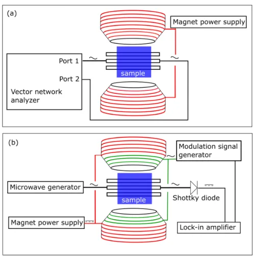
Two different FMR measurement setups were utilized for the experiments in this thesis, as illustrated in Fig. 2.2. Panel (a) sketches a Vector-Network-Analyzer (VNA) FMR setup. The VNA is connected to both ends of the CPW and acts as both the microwave source and detector, thus measuring all the scattering parameters Sab (a, b = 1,2) of the microwave circuit. As shown by Ding et al. [58] the measured S21 transmission parameter, measured from channel 1 to channel 2 of the VNA, carries both information about the magnetic and the non- magnetic characteristics of the microwave circuit, but in a constant-frequency- field-swept measurement the non-magnetic contribution toS21can be assumed to be a complex offset. Furthermore, thermal drifts or similar effects are accounted for by subtracting a complex linear background. Therefore, this discussion is limited to the ’magnetic’ ∆S21transmission parameter ∆S21=S21- offset - linear background.
The VNA measures the ∆S21parameter phase sensitive, in other words both the in phase components and the out-of-phase components of the signal, which for the magnetic signal correspond to the real and imaginary part of the complex susceptibility [52]. The VNA-FMR spectrum in the OOP geometry is therefore fitted with the following function:
∆S21(H0) =Aχzz(H0)eiφ, (2.10) whereAis a dimensionless amplitude andφ is the phase. Splitting up the fitting function into real and imaginary parts enables simultaneous fitting of both in- phase and out-of-phase components of ∆S21.
∆S21(H0) = Re (∆S21) +iIm (∆S21) (2.11) Re (∆S21) =
AMs(H0−Meff)
(H0−Meff)2−Heff2 cos (φ)−(2αHeff(H0−Meff)) sin (φ)
(H0−Meff)2−Heff2 + (2αHeff(H0−Meff))2
(2.12) Im (∆S21) =
AMs(H0−Meff)
(H0−Meff)2−Heff2 sin (φ) + (2αHeff(H0−Meff)) cos (φ)
(H0−Meff)2−Heff2 + (2αHeff(H0−Meff))2
(2.13)
Figure 2.2: Schematic of the FMR measurement setup. (a) depicts the VNA-FMR setup, where the sample and waveguide are placed in an external magnetic field and both ends of the waveguide are connected to the VNA. Then the ∆S21 transmission parameter between port 1 and 2 of the VNA is measured. The second measurement setup utilized in this thesis is schematically shown in (b). The microwave signal is generated by a microwave signal generator, transmitted through the waveguide and then converted into a DC signal via a Schottky diode, which is then detected by a lock- in amplifier. Modulation of the FMR signal is achieved by modulation of the external magnetic field via a set of modulation coils.
The second measurement setup, illustrated in Fig. 2.2 (b), utilizes a microwave generator connected to the waveguide as a microwave source. The other end of the waveguide is connected to a Schottky diode, which rectifies the microwave current. The diode signal is then measured via a lock-in amplifier for better signal to noise ratio. Low frequency modulation (≈86 Hz) of the signal is achieved by field modulation. Smaller modulation coils are attached to the pole shoes of the DC field magnet and a low frequency ac current is applied inducing a modulation field on the order of 100 Oe in direction of the fieldH0. The measured microwave signal is then proportional to derivative of the imaginary part of the microwave susceptibility [56] with respect to the external field. In an arbitrary measure- ment geometry the full microwave susceptibility can be rather complicated, but always exhibits Lorentzian lineshape [51, 59]. Therefore, the FMR spectra mea- sured by lock-in technique are simply fitted by a combination of symmetric and anti-symmetric Lorentzians differentiated with respect to the external magnetic field [57,59], taking the form,
S 2 (H0−Hres) ∆H2
∆H2+ (H0−Hres)22 +I8∆H(H0−Hres)2−4∆H3
∆H2+ (H0−Hres)22 . (2.14) S and I are the amplitudes of symmetric and antisymmetric Lorentzian respec- tively. Hreshere carries all information on the magnetic anisotropy, as anisotropy is not explicitly included in the fitting function. All anisotropies then can be determined by measuring Hres angle dependent [56].
Errors for all fitting parameters are determined by 1σ (95 %) confidence intervals of the fits. These errors are then used as weights for fitting Eqs. (2.3) and (2.4) to the resonance field and linewidth data. The spectroscopic g-factor g and the effective magnetizationMeff are the fitting parameters in Eq. (2.3), and the inho- mogeneous linewidth broadening ∆H0 and the dampingα are fitting parameters in Eq. (2.4). The fitting errors to these parameters are again determined by 95 % confidence intervals of the fits, thus assigning reasonable errors to the extracted determined material parameters.
3
Gilbert-like Damping
The focus of this thesis lies on the measurement of Gilbert-like damping mech- anisms, i.e. damping mechanisms leading to a linear dependence of linewidth on frequency. In the previous chapter damping was only introduced as a phe- nomenological parameter to describe the relaxation of an excited magnetization vector towards the equilibrium position and to quantify the linewidth of FMR spectra. In this chapter the physical origins of multiple damping mechanisms will be discussed. The contributions to the experimentally determined damp- ing are commonly divided into two categories: intrinsic damping and extrinsic contributions to the damping [50]. As this distinction is often misleading, only the damping directly correlated to intrinsic material properties, will be called intrinsic damping. In other words, only the damping that cannot be influenced or determined by sample or measurement geometry will be called intrinsic damp- ing. Damping mechanisms that can be influenced by sample or measurement geometry will be called extrinsic damping.
3.1 Intrinsic damping
Even in a perfectly crystalline ferromagnet the magnetic precession will not be free of damping. Many theoretical approaches state that this is due to spin-orbit- coupling (SOC), a purely quantum mechanical effect that couples spin and orbital moments [51]. The SOC enables transfer of energy from the spin system to the electronic system, thus opening a channel for energy dissipation from the spin precession. In combination with other equilibration processes of the electronic system, this leads to a damping of the precession.
One of the goals of the theoretical description of the damping is to correctly model the experimentally found temperature dependence of the damping in metallic fer- romagnets [60, 62]. An example of this behavior is shown in Fig. 3.1, depicting both an increase of the damping towards low and towards high temperatures.
This behavior closely correlates to the behavior of the conductivity at low tem- peratures and the behavior of the resistivity at high temperatures and is therefore
Figure 3.1: From Ref. [60] and references therein. Collected data for the temperature variation of the Landau relaxation frequency λ(λ∝α, compare Ref. [61]) for Fe, Co, Ni, and NiCu alloys.
also called conductivity-like and resistivity-like, respectively.
More recently numerical calculations of values for the damping and both temper- ature dependence and alloy composition dependence have been published [43,63, 64]. In the following sections a short overview of the most prominent approaches and their numerical results will be given.
3.1.1 Breathing and bubbling Fermi surface models
One of the early successful theories describing the conductivity-like low tem- perature behavior of the damping was that of Kamberský, who introduced the so-called breathing Fermi surface model (BFS) [65, 66]. In the BFS model the damping term (in Landau-Lifshitz notation λ, compare Ref. [61]) is written as
λ= g2µ2B
~
X
n
Z dk3
(2π)3η(n,k) ∂n,k
∂θ
!2
τl
~
. (3.1)
The name breathing Fermi surface stems from the picture that the precessing magnetization, due to spin-orbit coupling, distorts the Fermi surface, as modeled in Eq. (3.1) by variations of the single particle states ∂n,k with the spin direc- tion θ. n and k are labeling band index and wave vector, respectively. η(n,k) is the negative derivative of the Fermi function only allowing states near the Fermi energy to contribute to the damping. The distortion of the Fermi surface
causes some populated states to rise above the Fermi energy and pushes some unpopulated states below, creating electron-hole pairs near the Fermi surface.
Recombination of the electron-hole pairs is delayed by the lifetime τ, which in this way governs the equilibration of the system. A short scattering time (high temperature) will cause a quick equilibration of the distorted Fermi surface and therefore lower damping. However, for long life times a stronger distortion of the Fermi surface is induced and a stronger damping is expected. Therefore, the damping scales with τl.
When comparing the predictions of the BFS model to experimental findings, good qualitative agreement for the low temperature (largeτl) behavior of the damping is found, compare Fig. 3.1. However, the BFS fails in describing the resistivity- like increase of the damping at higher temperatures.
Therefore a different mechanism has to be responsible for this behavior. Heinrich, et al. [67] described this mechanism in the so called bubbling Fermi surface model or s-d exchange model. This model is based on the interaction of localized d- states with itinerant s-p states. Strictly speaking, there is no clear distinction between s-p and d states in 3d transition metals, due to s-p hybridization and d- band delocalization [68,69] of differing degrees, but the distinction here serves to describe electrons of localized and itinerant character. The interaction between s and d electrons enables a scattering between magnons and itinerant electrons, resulting in the creation and annihilation of electron-hole pairs. The magnon gets annihilated in the scattering process, which therefore entails a spin-flip, due to angular momentum conservation. s-d scattering alone does not dissipate angular momentum from the magnetic system, as it only changes the occupation of the bands. Only in combination with additional scattering processes, which recombine the electron-hole pairs, angular moment dissipation in the magnetic system can occur. The damping in the s-d model can be written as [50,57]
α= µ2BN(EF) Msγ
1
τl, (3.2)
whereN(EF) is the density of states at the Fermi energy andτl is the interband electron-hole lifetime time. From this equation it is obvious that the damping caused by s-d interaction increases with increasing temperature (small τl), thus describing the high temperature behavior of the damping.
A note of caution is necessary at the end of this section, since the lifetimes τl for the BFS and the s-d models are not automatically the same. The strength of different scattering mechanisms, such as electron-electron or electron-phonon scattering, limiting the lifetimes of electron-hole pairs, depend on the exact band structure and can therefore differ for the electron-hole pairs produced in the two different scattering processes. Nevertheless, the lifetimes always are proportional to the momentum scattering time τ, and can be approximated by it.
3.1.2 Torque correlation model
In order to describe the damping over the whole temperature range Kamber- ský [29] introduces his so-called torque-correlation model. In the torque correla- tion model the damping can be written as [27]
λ= g2µ2B
~
X
n,m
Z dk3 (2π)3
Γ−n,m
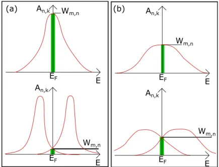
2Wnm(k), (3.3) where Γ−n,m = hn, k|[σ−, HSO]|m, ki are the matrix elements for the SOC medi- ated transition between state m and n andWnm(k) = (1/τ)R dωη(ω)An,k(ω)Am,k(ω) describes the spectral overlap of the electron spectral functions Am/n,k at the Fermi Energy. Am/n,k are modeled as Lorenzian functions with width ∝ ~/τ around the center of the band.
Qualitatively Eq. (3.3) describes the decay of magnons into electron-hole pairs, mediated by SOC. The electron-hole pairs can either occupy the same band or two different spin split bands, i.e the spin-flip scattering can occur intra- or inter- band. The intra-band spin flip scattering only is non-zero due to a mixing of both spin states in one band, caused by the SOC.
E EF
Wm,n
EF E
Wm,n An,k
An,k
E EF
Wm,n
EF E
Wm,n An,k
An,k
(a) (b)
Figure 3.2: Illustration of the spectral overlap function Wnm. (a) and (b) show spectral functions Am/n,k for intra and inter band scattering with small (large τ) and large (smallτ) width, respectively. The width of the spectral functions is shown by the blue lines and Wnm is signified by the green areas. Adapted from Ref. [61].
The spectral overlap function at the Fermi energyWnmexhibits different behavior for intra- and inter-band transitions. In the case of intra-band transitions, Wnm
is approximately the amplitude of the Lorenzian spectral function at the Fermi energy. Thus, Wnm scales inversely with the width of the spectral function and therefore scales directly with the scattering time τ. For an inter-band scattering event Wnm describes the overlap between two energetically shifted electron spec- tral functions at the Fermi energy. Wnm now scales with the width of the spectral functions (∝1/τ). An illustration of Wnm for the two different cases is shown in Fig. 3.2. Thus, it can be concluded that Eq. (3.3) qualitatively describes both resistivity and conductivity like behavior of the damping. As shown in Ref. [27]
the intra-band terms of Eq. (3.3) describe the same physics as the BFS model in the long scattering time limit.
Figure 3.3: From Ref. [27]. The dependence of the damping param- eter on the inverse scattering time 1/τ is shown for Ni, Fe and Co (solid lines). The dotted lines rep- resent the inter-band contributions and the dashed lines the intra-band contributions. For all elements the damping displays a distinct mini- mum for different scattering times.
Due to the taxing computational requirements for quantitative predictions by this model only limited quantitative analysis was pub- lished [65] until more recently Gilmore, et al.[27], as well as Thonig,et al. [70] computed values of the damping based on the torque- correlation model for the 3d transition metals Ni, Co and Fe, as shown in Fig. 3.3.
The calculated damping depends on the mo- mentum scattering time τ. For longer τ the damping increases, because the intra- band scattering contribution to the damp- ing dominates, causing a damping enhance- ment. Similarly, for shorter τ the inter-band contribution dominates, enhancing the damp- ing. Therefore the damping exhibits a min- imum in 3d transition metals at a element specific τ, when both intra- and inter-band contributions are of roughly similar magni- tude. These calculations model the temper- ature dependence of the damping reasonably well, but quantitative comparison to mea- surements is complicated due to difficulties in the exact determination of the momen- tum scattering time. This reliance on τ is a large obstacle for a quantitative anal- ysis. Nevertheless, the torque correlation model delivers a good qualitative description of the temperature dependent behavior of the damping and can be a rather intuitive tool for materials engineering of the damp- ing.
3.1.3 Scattering matrix approach
Another approach for the calculation ofαintvia scattering theory was successfully implemented by Brataas,et al.[30], which is a generalization on non-local interfa- cial damping enhancement, i.e. spin pumping (discussed in Sec. 3.2.3). However, intrinsic spin relaxation can also be included in the scattering matrix formalism.
The calculations are based on the model of a ferromagnet in contact to a thermal bath via normal metal leads. The precession of the magnetization heats up the ferromagnetic system and this excess heat leaks via the normal metal contacts, thus dissipating energy from the magnetic system. The energy pumping into the normal metal leads can be described in a scattering matrix (Sij) formalism, accounting for reflexion and transmission at the interfaces. Comparison of this energy flux to the energy dissipation term in the LLG results in an expression for the damping tensor ˜Gij, which depends on the scattering matrix:
G˜ij = γ2~
4π Re Tr
"
∂S
∂m˜i
∂S†
∂m˜j
#!
, (3.4)
where ˜mi and ˜mj are the components of the normalized magnetization vector
˜
m = m/Ms. The expression for the intrinsic damping in the scattering ma- trix approach is qualitatively similar to the one derived in the torque-correlation model [30]. But the scattering matrix approach allows simultaneous and sepa- rable determination of bulk-damping and spin pumping contribution, by includ- ing spin-flip scattering in the scattering matrix. Assuming isotropic damping G˜ij) = ˜G), and the total damping for a sample with thickness t can be written as ˜G(L) = ˜Ginterface + ˜Gbulk(t), where ˜Ginterface is the interfacial damping term, which is constant in this approach and ˜Gbulk(t) is the thickness dependent bulk damping,which can be expressed as ˜Gbulk(t) = αγMs(t). The Gilbert damping parameter is then extracted from the slope of ˜Gbulk(t) vs. t, as demonstrated in Ref. [63].
3.1.4 Numerical calculations of the damping
Over the last two decades the development of powerful computational and theo- retical methods (density functional theory, DFT) allowed detailed calculations of the electronic band structure. Based on these band structure calculations various approaches to quantitatively model the damping in 3d transition metals and their alloys have been published. The following paragraph is intended as an overview
of the calculations that experimental results are compared to in this thesis, with no claim for completeness.
A numerical estimate of the damping of Fe and Ni in the linear response model was performed by Kamberský himself [71]. Similarly Gilmore,et al. [27], as well as Thonig,et al. [70] calculated the damping for Ni, Fe and Co in a torque corre- lation model. Both of these approaches specify the SOC as the main mechanism for the damping, but do not describe mechanisms for the spin flip scattering, necessary to dissipate angular momentum from the system. Both models rely on artificially introduced parameters to model the electron life time. Therefore, these calculations yield the damping only as a function of the momentum scatter- ing time. This problem was first addressed by Brataas,et al.[30], who described the damping via scattering theory, allowing Starikov, et al. [63] a first princi- ples calculation of the damping of NiFe alloys, which was expanded by Liu, et al. [72] to include the influence of electron-phonon interaction on the damping.
Furthermore, this formalism was applied for the calculation of the damping in non-collinear ferromagnetic systems, i.e. domain walls [73]. Another first prin- ciples approach was achieved by a numerical realization of Kamberský’s linear response model [65] performed by Ebert, et al. [26] for NiFe. Later Mankovsky, et al. [43] expanded the calculations for NiCo, NiFe, FeV and CoFe alloys. The latter work includes calculations of the dependence of the damping on tempera- ture for Ni, Fe, and Co, making it a comprehensive theoretical study of binary alloy properties and will be the main study to compare experimental values to in this thesis. More recently Turek,et al. [64] calculated the damping for NiFe and CoFe alloys in the torque-correlation model, utilizing non-local torque correlators, thus archiving an ab initio description of the damping in those systems.
3.2 Extrinsic Contributions to the total measured damping
The methods for the calculation of the damping described in the previous sections only account for the intrinsic damping of the ferromagnet. Experimentally deter- mined damping will often consist of multiple extrinsic contributions additional to the intrinsic damping [74]. Hence, the extrinsic contributions to the damp- ing need to be identified and quantified in any experiment in order to facilitate a comparison of experimentally determined damping to calculated values. This chapter introduces several mechanisms for extrinsic contributions to the damping and how to experimentally determine them.
3.2.1 Radiative damping
The model and experimental results presented in this section have been published in Ref. [46].
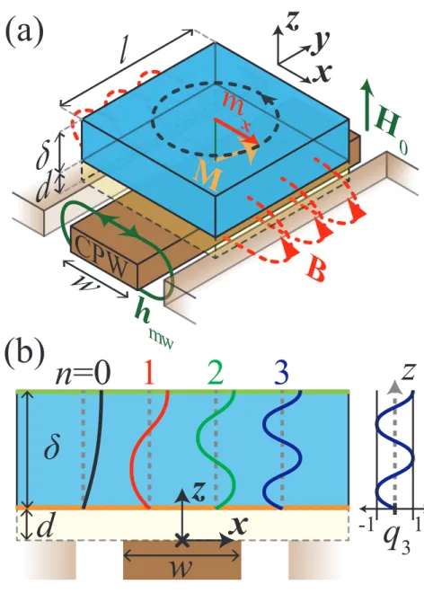
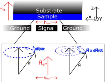
According to Faraday’s Law, the time-varying flux of a precessing magnetic mo- ment generates an ac voltage in any conducting material that passes through the flux. As shown in Fig. 3.4, spin wave precession in a conducting ferromagnet on top of a coplanar waveguide (CPW) induces ac currents both in the ferromagnet and the CPW. The dissipation of these eddy currents in the sample, and the flow of energy away in the CPW give rise to two contributions to magnetic damping.
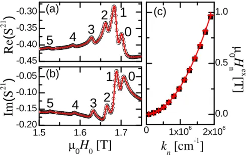
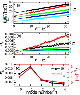
Historically, the damping caused by eddy currents in the ferromagnet αeddy is called eddy current damping, while the damping caused by the eddy currents in the waveguide is called radiative damping αradn . This section will describe an an- alytical model for radiative damping. The validity of this model is supported by damping measurements of perpendicular standing spin waves (PSSWs) in Permal- loy films.
3.2.1.1 Radiative damping model
In a experimental geometry as sketched in Fig. 3.4 (a), a ferromagnetic sam- ple with thickness δ and length l is placed on top of the center conductor of a coplanar waveguide (CPW) with width W. The sample dimension along x is much larger than W. The sample and CPW are separated by a gap of height d. An external DC magnetic field H0 is applied perpendicular to the sample plane, and the spin wave resonances (SWR) are driven by microwaves in the CPW at resonance frequency f. A fraction of the ac magnetic induction B due to the
dynamic component of the magnetization mxn(H0, I;z) wraps around the center conductor.
To derive a quantitative expression for αradn , we start by calculating hx(I;x, z), the x component of the driving field hmw that is generated by an excitation currentI in the center conductor. We assumehx(I;x, z) is uniform along y, but we allow for variation alongxandz. To estimatehx(I;x, z) we use the Karlqvist equation [75]
hx(I;x, z) = I 2πW
"
arctan x+W/2 z
!
−arctan x−W/2 z
!#
. (3.5)
This microwave field can excite PSSWs in the sample. Schematic mode profiles for the fundamental mode (n= 0) and the first three PSSW modes are shown in Fig. 3.4(b), where arbitrarily unpinned boundary conditions at the top surface and pinned boundary conditions at the bottom surface were chosen.
The mode profiles describe a z-dependence of the dynamic magnetization com- ponents mx and my. In the perpendicular geometry used here, |mx| = |my| everywhere, i.e. the precession is circular. In what follows, only mx, the dy- namics of which are inductively detected in the measurement, will be discussed.
Furthermore, the analysis is restricted to the case of ideal perpendicular standing spin wave modes in a fully saturated film that only vary through the film thick- ness without any lateral variation. This eliminates the need to explicitly consider the full Polder susceptibility tensor in the calculation of the sample response to the excitation field. The sample dimensions arel along the waveguide direction, δ in thickness, but infinite in the lateral direction.
Introducing the concepts of a spin wave mode susceptibility χn, and the dimen- sionless, normalized spin wave amplitude qn(z) for the nth spin wave mode, the magnetic excitation of amplitude in x-direction ˜mxn(H0, I;z) that results from the application of a microwave magnetic field of amplitude hx(I;x, z), driven by an ac currentI =Vin/Z0 in an applied field H0 can be written as
˜
mxn(H0, I;z) := ˜mxn(z) = qn(z)χn(H0)hqn(z)hx(I;x, z)i (3.6) where the quantity in brackets is simply the overlap integral of the excitation field and the normalized spatial profile of the nth spin wave mode qn(z). The magnetic excitation of amplitude iny-direction ˜myn(z) can be written in a similar way. In the trivial case of a uniform excitation field and uniform spin wave mode, we recover the usual relation between the excitation field and the magnetization dynamics via the Polder susceptibility tensor component, χxx. However, if the product of the mode profile and excitation field has odd spatial symmetry, dy- namics are not excited, as we expect. The overlap integral is nothing more than
n=0 1 2 3
z x d w
δ
q 3 1
-1
z H 0
M m x
B d
l δ
x y z
w CPW
(a)
(b) h
mw
Figure 3.4: Schematic of the radiative damping process. (a)M is the dynamic mag- netization, H0 the applied external field andB is the magnetic inductance due to the x-componentmx of the dynamic magnetization. W is the width of the center conduc- tor, l the length of the sample on the waveguide, δ the thickness of the sample and d the spacing between sample and wave guide. (b) Simplified depiction of the PSSW eigenfunctions qn for mode numbers n= 0, 1, 2, 3. We exemplary used boundary con- ditions that are completely pinned on one side and completely un-pinned on the other side. The origin of the coordinate system is indicated.
the spatial average of the mode/excitation product:
hqn(z)hx(I;x, z)i= 1 W δ
Z ∞
−∞dx
Z δ+d d
dzqn(z)hx(I;x, z). (3.7) The power transferred to the waveguide via inductive coupling with the spin wave dynamics is given by
Pn= |∂tΦn(H0, I)|2
2Z0 , (3.8)
where
∂tΦn(H0, I) = µ0`
∞
Z
−∞
dx
δ+dZ
d
dz(∂tmxn(z)) ˜hx(x, z), (3.9)
with ˜hx(x, z) = hx(I;x, z)/I.
It is important to recognize at this point that the power dissipation is not constant with time, given that Pn is proportional only to ∂tmxn. As such, the damping associated with the re-radiation of the microwave energy back into the waveguide is best characterized with an anisotropic damping tensor, to be elaborated upon in more detail later in this section. To calculate the energy of the spin wave mode a spatially averaged spin wave excitation density [76] is defined,
Dµ2n(H0, I)E =
R∞
−∞dxRdδ+ddz[(∂tmxn(z)) (myn(z))∗ −(∂tmyn(z)) (mxn(z))∗]
4ωδW .
(3.10) Then, the magnon densityNn associated with the nth spin wave excitation is
Nn = hµ2n(H0, I)i
2gµBMs (3.11)
And the total energy associated with the spin wave mode is given by
En = ωhµ2n(H0, I)i
γMs δ`W (3.12)
The energy dissipation rate (1/T1)n for the nth mode is therefore
1 T1
n
= Pn
En = 2µ0`ωM
Z0
∞
R
−∞
dxδ+dR
d
dz(∂tmxn(z)) ˜hx(x, z)
2
∞
R
−∞
dx
δ+d
R
d
dzh(∂tmxn(z)) (myn(z))∗−(∂tmyn(z)) (mxn(z))∗i ,
(3.13) where ωM =γµ0Ms. Applying the Fourier transform to move into the frequency domain, where ∂tmxn(H0, I;z)↔iωm˜xn(H0, I;z), such that the energy relaxation rate (1/T1)xn for magnetization oscillations along the x-axis is written as
1 T1
x n
= ωµ0`ωM
Z0 Kn, (3.14)
where
Kn :=
∞
R
−∞
dxδ+dR
d
dz( ˜mxn(z)) ˜hx(x, z)
2
∞
R
−∞
dx
δ+d
R
d
dzIm [ ˜mxn(z) ( ˜mxn(z))∗] (3.15) is a dimensionless inductive coupling parameter. In the limiting case of then= 0 (i.e., uniform) mode with a uniform excitation field due to current flowing only through the waveguide center conductor, and an infinitesimal spacing between the waveguide and the sample, we have K0 =δ/4w. Substituting Eq. (3.6) into Eq. (3.15), the general result
Kn=
∞
R
−∞
dxδ+dR
d
dzqn(z) ˜hx(x, z)
2
δ+dR
d
dz|qn(z)|2
, (3.16)
is obtained, with =|m˜zn|/|m˜xn|.
Since the energy dissipation rate for the case of radiative damping is anisotropic, it must be generally treated in the damping tensor formalism, where the Gilbert damping torque T is given by
Tk=εijkαijmˆi(∂tmˆ)j. (3.17) The equation of motion is given in form of a LLG
∂tmˆ =−γµ0mˆ ×H+T (3.18) and ˆm=M/Msis the normalized magnetization. For the coordinates in Fig 3.4, the only nonzero radiative damping tensor components areαzx and αyx. For the perpendicular FMR geometry, the relationship between the energy relaxation rate and the Gilbert damping components is
1 T1
x
=αzxωx, (3.19)
and
1 T1
y
=αzyωy, (3.20)
whereωx and ωy are the respective stiffness frequencies, defined as
ωi := γ Ms
∂2Um
∂mˆi (3.21)
and Um is the magnetic free energy function. The frequency-swept linewidth
∆ω =γµ0∆H, where ∆H is the field-swept linewidth in Eq. (3.40), is given by
∆ω=
1
T1
x
+T11y
2 (3.22)
=αzxωx+αzyωy (3.23)
For perpendicular FMR,ωx =ωy =ω, and the specific case of anisotropic radia- tive damping, αzx=αradn , αzy = 0,
αradn = 1 2ω
1 T1
x n
= µ0lωM
2Z0 Kn (3.24)
and ∆ωnrad =αnradω. This is in contrast to the case of isotropic damping processes, such as eddy currents and intrinsic damping, where ∆ωniso = 2αison ωinstead. Thus, the net damping due to the sum of anisotropic radiative damping, and any other isotropic processes, is given by
αn =αisotropic+αradn
2 (3.25)
![Figure 3.1: From Ref. [60] and references therein. Collected data for the temperature variation of the Landau relaxation frequency λ ( λ ∝ α , compare Ref](https://thumb-eu.123doks.com/thumbv2/1library_info/4131974.1552116/20.892.262.652.175.473/figure-references-collected-temperature-variation-landau-relaxation-frequency.webp)