Well−Structured Transition Systems Everywhere !

A. Finkel and Ph. Schnoebelen

Well−Structured Transition Systems Everywhere !

Research Report LSV−98−4, Apr. 1998

Ecole Normale Supérieure de Cachan

61, avenue du Président Wilson

http://www.lsv.ens−cachan.fr/Publis/

Research Report LSV−98−4, Lab. Spécification et Vérification, CNRS & ENS de Cachan, France, Apr. 1998

An updated version will appear in Theoretical Computer Science. See WWW publications pages of the authors.

Well-Structured Transition Systems Everywhere !

A. Finkeland Ph. Schno eb elen

Lab. Sp ecication and Verication

ENS de Cachan &CNRS URA2236

61, av. Pdt Wilson; 94235 Cachan Cedex; FRANCE email:

nkel,phs

@lsv.ens-cachan.fr

April 7,1998

Abstract

Well-structured transition systems (WSTS's) are a general class of innite state systems for which decidability results rely on the existence of a well-quasi-ordering between states that is compatible with the transitions.

In this article, we provide an extensive treatment of the WSTS idea and show several new results. Our improved denitions allow many examples of classical systems to be seen as instances of WSTS's.

1 Introduction

Verication of innite-state systems. Formal verication of programs and systems is a very active eld for both theoretical research and practical developments, especially since im- pressive advances in formal verication technology proved feasible in several realistic appli- cations from the industrial world. The highly successful model-checking approach for nite systems [BCM

92] suggested that a working verication technology could well be developed for systems with an innite state space.

This explains the considerable amount of work that has been devoted in recent years to this

\verication of innite state systems" eld, with a surprising wealth of positive results [Mol96, Esp97]. The eld now has its own conference.

Well-structured transition systems. A very interesting development in this eld is the introduction of well-structured transition systems (WSTS's). These are transition systems where the existence of a well-quasi-ordering over the innite set of states ensures the termination of several algorithmic methods. WSTS's are an abstract generalization of several specic structures and they allow general decidability results that can be applied to Petri nets, lossy channel systems, and many more. (Of course, WSTS's are not intended as a general explanation of all the decidability results one can nd for specic models.)

Finkel [Fin87a, Fin87b, Fin90] was the rst to propose a denition of WSTS (actually several

variant denitions). His insights came from the study of Petri nets where several decidability

results rely on a monotonicity property (transitions rable from marking M are rable from any

larger marking) and Dickson's lemma (inclusion between markings of a net is a well-ordering). He

mainly investigated the decidability of termination, boundedness and coverability-set problems.

He applied the idea to several classes of fo nets and of CFSM's (see Section 9).

Independently, Abdulla et al. [ACJY96] later proposed another denition. Their insights came from their study of lossy-channel systems and other families of analyzable innite-state systems (e.g. integral relational automata [Cer94]). They mainly investigated covering, in- evitability and simulation problems. They applied the idea to timed networks [AJ97] and lossy systems.

Later, Kushnarenko and Schnoebelen [KS97a] introduced WSTS's with downward compati- bility, motivated by some analysis problems raised by Recursive-Parallel Programs.

Some criticisms. Though the two earlier lines of work had a great unifying power, they still suered from some defects (these defects are also present in [KS97a]).

Both Finkel and Abdulla et al. proposed denitions aiming at a specic algorithm or two, hence their WSTS concept is burdened with unnecessary structure. Finkel was interested in coverability-sets, so that his denition included e.g. complex continuity requirements.

Abdulla et al. were interested in simulation with a nite state system, so that their denition included e.g. labels on transitions.

More generally, both denitions are conservative for no good reason we can think of. As a consequence, both proposals end up surprisingly short of simple examples of their \general"

concept.

Both denitions mix up structural and eectiveness issues while in reality the eectiveness requirements are quite variable, depending on which algorithm one is talking about. As a result their denition becomes more complex and restrictive when more decision methods for WSTS's are found.

Several proofs in these earlier papers are quite messy or tedious. In part this is due to the unnecessarily complex denitions and to a lack of classifying work. As a consequence some potentially enlightening connections are hard to notice.

These early works do not tackle the fundamental question of \how / when can one turn a given (family of) transition system into WSTS ?", i.e. how can one nd a compatible well-ordering ?

Our contribution. This article is both a survey of earlier works on the WSTS idea, and a presentation of our proposal for a new conceptual framework, together with several new results or new extensions of earlier results.

More precisely,

We propose and investigate a cleaner, more general denition of WSTS, generalizing the early insights of Finkel, Abdulla et al., Kushnarenko and Schnoebelen.

We separate structural and eectiveness issues and only add eectiveness hypothesis when and where they are needed for a decision method.

We classify the decision methods into two main families: set-saturation and tree-saturation

methods.

We give ve main decidability results. Except for Theorem 5.5, they never appeared in such a general framework. Both Theorem 3.6, made possible by our Denition 3.2, and Theorem 4.8, made possible by the key notion of stuttering compatibility, have much more applications than their ancestors.

We give a quite large collection (summarized in Fig. 9, page 26) of system models that can be tted into the WSTS framework. These examples come from various elds of computer science. Many have not been noticed earlier. Several of them use original and innovative well-orderings. Roughly half of them are WSTS's only in our new, generalized, denition.

Finally, we ask how and when a given transition system can be given a well-structure.

We oer surprisingly general answers (e.g. our Ubiquity Theorem) for the more liberal denition.

Outline of the article. This article is divided into three parts. In Part I we introduce the fundamentals concepts underlying WSTS's (section 2) and we describe the two main families of decision methods for WSTS's: set-saturation methods (section 3) and tree-saturation methods (section 4). We conclude this part with downward-WSTS's (section 5).

Part II is devoted to examples of WSTS's. We successively visit Petri nets and their exten- sions (section 6), string rewrite systems (section 7), process algebra (section 8), communicating automata (section 9) and a few less classical operational models of computation (section 10).

All these (families of) models are found to be well-structured in natural ways. This is a strong point in favor of our claim that we propose a more interesting denition of WSTS's.

Finally, Part III is concerned with the passage from TS's to WSTS's. We investigate when and how does there exist well-quasi-orderings that can provide a well-structure to a given transition system.

Part I

Fundamentals of WSTS's

Part I presents the technical core of the WSTS idea. As a rule, examples and illustrations have been postponed until Part II.

2 Basic notions

2.1 Well-quasi-orderings

Recall that a quasi-ordering (a qo) is any reexive and transitive relation

. We let x < y denote x

y

x . A partial ordering (a po, an \ordering", ::: ) is an antisymmetric qo. Any qo induces an equivalence relation ( x

y i x

y

x ) and gives rise to a po between the equivalence classes.

We now need a few results from the theory of well-orderings (see also e.g. [Kru72, Hig52]).

Denition 2.1. A well-quasi-ordering (a wqo) is any quasi-ordering

(over some set X ) such

that, for any innite sequence x

;x

;x

;::: in X , there exists indexes i < j with x i

x j .

Hence a wqo is well-founded, i.e. it admits no innite strictly decreasing sequence x

> x

>

x

>

Lemma 2.2. (Erdos & Rado) Assume

is a wqo. Then any innite sequence contains an innite increasing subsequence: x i

x i

x i

::: (with i

< i

< i

::: ).

Proof. Consider an innite sequence and the set M =

i

j > i;x i

x j

. M cannot be innite, otherwise it would lead to an innite subsequence contradicting the wqo hypothesis.

Thus M is bounded and any x i with i beyond M can start an innite increasing subsequence.

Given

a quasi-ordering, an upward-closed set is any set I

X such that y

x

I entails y

I . To any x

X we associate

x

=

y

y

x

. It is upward-closed. A basis of an upward-closed I is a set I ^b such that I =

_x

_I b

x . Higman investigated ordered sets with the nite basis property.

Lemma 2.3. [Hig52] If

is a wqo, then any upward-closed I has a nite basis.

Proof. The set of minimal elements of I is a basis because

is well-founded. It only contains a nite number of non-equivalent elements otherwise they would make an innite sequence contradicting the wqo assumption.

Lemma 2.4. If

is a wqo, any innite increasing sequence I

I

I

of upward-closed sets eventually stabilizes, i.e. there is a k

such that I k = I k

= I k

= :::

Proof. Assume we have a counter-example. We extract an innite subsequence where inclusion is strict: I n

I n

I n

. Now, for any i > 0, we can pick some x i

I n _i

I n _i

. The well-quasi-ordering hypothesis means that the innite sequence of x i 's contains an increasing pair x i

x j for some i < j . Because x i belongs to an upward-closed set I n i we have x j

I n i , contradicting x j

I n j

.

2.2 Transition systems

A transition system (TS) is a structure

=

S;

;:::

where S =

s;t;:::

is a set of states, and

S

S is any set of transitions. TS's may have additional structure like initial states, labels for transitions, durations, causal independence relations, etc., but in this paper we are only interested in the state-part of the behaviors.

We write Succ ( s ) (resp. Pred ( s )) for the set

s

S

s

s

of immediate successors of s (resp.

s

S

s

s

the predecessors). A state with no successor is a terminal state. A computation is a maximal sequence s

s

s

of transitions.

We write

ⁿ (resp.

,

,

) for the n -step iteration of the transition relation

(resp. for its transitive closure, for its reexive closure, for its reexive and transitive closure). Hence

is

. We use similar notation for Succ and Pred , so that for

+ ; = ;

; 0 ; 1 ; 2 ;:::

, Succ ( s ) is

s

s

s

.

S

is nitely branching if all Succ ( s ) are nite. We restrict our attention to nitely branching

TS's.

2.3 Well-structured transition systems

Denition 2.5. A well-structured transition system (WSTS) is a TS

=

S;

;

equipped with a qo

S

S between states such that the two following conditions hold:

(1) well-quasi-ordering:

is a wqo, and

(2) compatibility:

is (upward) compatible with

, i.e. for all s

t

and transition s

s

, there exists a sequence t

t

such that s

t

.

Thus compatibility states that

is a weak simulation relation a la R. Milner.

See Figure 1 for a diagrammatic presentation of compatibility where we quantify universally over solid lines and existentially over dashed lines. Several families of formal models of processes

PSfrag replacements

8

9

s

s

t

t

Figure 1: (Upward) compatibility

give rise to WSTS's in a natural way, e.g. Petri nets when inclusion between markings is used as the well-ordering. In Part II, we shall see many more examples.

3 Set-saturation methods

We speak of set-saturation methods when we have methods whose termination relies on Lemma 2.4.

In this section, we illustrate the idea with backward reachability analysis, generalizing a result from [ACJY96].

Other examples of the set-saturation family are the algorithm for simulation by a nite state system (from [ACJY96]), and the algorithm for the sub-covering problem (from [KS97a]).

Assume

=

S;

;

is a WSTS and I

S is a set of states. Backward reachability analysis involves computing Pred

( I ) as the limit of the sequence I

I

::: where I

= I and I n

= I n

Pred ( I n ). The problem with such a general approach is that termination is not guaranteed. For WSTS's, this can be solved when I is upward-closed:

Proposition 3.1. If I

S is an upward-closed set of states, then Pred

( I ) is upward-closed.

Proof. Assume s

Pred

( I ). Then s

t for some t

I . If now s

s then upward- compatibility entails that s

t

for some t

t . Then t

I and s

Pred

( I ).

Pred

( I ) can be computed if we make a few decidability assumptions:

Denition 3.2. A WSTS has eective pred-basis if there exists an algorithm accepting any

state s

S and returning pb ( s ), a nite basis of

Pred (

s ).

Note that Denition 3.2 is distinct from the requirement for a basis of Pred (

s ) used in [ACJY96]. Our denition is necessary for the generalized Theorem 3.6 we aims at.

Now assume that

is a WSTS with eective pred-basis. Pick I ^b a nite basis of I and dene a sequence K

;K

;::: of sets with K

= I ^b , and K n

= K n

pb ( K n ). Let m be the rst index such that

K m =

K m

. Such an m must exist by Lemma 2.4.

Lemma 3.3.

K m =

_i

K i .

Proof. This is not a consequence of Lemma 2.4 but rather of

"

Y =

Y

implies

pb ( Y ) =

pb ( Y

) :

which relies on the denition of pb and the distributivity property of Pred and

w.r.t. union.

Lemma 3.4.

K i = Pred

( I ).

Proof. Use induction over n and show that

K n

K n

Pred

( I ) (=

Pred

( I ))

On the other hand, the denition of pb entails

Pred ⁿ ( I )

K n , so that Pred

( I )

i

"

K i

[

i

K i

Pred

( I ) :

Proposition 3.5. If

is a WSTS with (1) eective pred-basis and (2) decidable

, then it is possible to compute a nite basis of Pred

( I ) for any upward-closed I given via a nite basis.

Proof. The sequence K

;K

;::: can be constructed eectively (each K n is nite and pb is eective). The index m can be computed because the computability of

entails the decidability of \

K =

K

?" for nite sets K and K

. Finally, K m is a computable nite basis of Pred

( I ).

The covering problem is to decide, given two states s and t , whether starting from s it is possible to cover t , i.e. to reach a state t

t .

The covering problem is often called the \control-state reachability problem" when S has the form Q

D (for Q a nite set of so-called \control states") and ( q;d )

( q

;d

) entails q = q

.

Theorem 3.6. The covering problem is decidable for WSTS's with (1) eective pred-basis and (2) decidable

.

Proof. Thanks to Proposition 3.5, one can compute K , a nite basis of Pred

(

t ). It is possible to cover t starting from s i s

K . By decidability of

, it is possible to check whether s

K .

Variants of this problem can be decided in the same way. E.g. deciding whether t can be covered

from all states in a given upward-closed I . Or from all states in a downward-closed D = S

I (this

requires WSTS's with intersection-eectiveness, i.e. there is an algorithm computing inter ( s;s

),

a nite basis of

s

s

).

4 Tree-saturation methods

We speak of tree-saturation methods when we have methods representing (in some way) all possible computations inside a nite tree-like structure. In this section, we illustrate the idea with the Finite Reachability Tree and its several applications to termination, inevitability, and boundedness problems.

Other examples of the tree-saturation idea is the algorithm for simulation of a nite state systems (from [ACJY96]), and the algorithm for coverability-sets (from [Fin87a]).

We assume

=

S;

;

is a WSTS.

4.1 Finite reachability tree

Denition 4.1. [Fin90] For any s

S , FRT ( s ), the Finite Reachability Tree from s , is a directed unordered tree where nodes are labeled by states of S . Nodes are either dead or live.

The root node is a live node n

, labeled by s (written n

: s ). A dead node has no child node. A live node n : t has one children n

: t

for each successor t

Succ ( t ). If along the path from the root n

: s to some node n

: t

there exists a node n : t ( n

= n

) such that t

t

, we say that n subsumes n

, and then n

is a dead node. Otherwise, n

is live.

Thus leaf nodes in FRT ( s ) are exactly (1) the nodes labeled with terminal states, and (2) the subsumed nodes. See Part II for examples.

Lemma 4.2. FRT ( s ) is nite (hence the name).

Proof. The wqo property ensures that all paths in FRT ( s ) are nite because an innite path would have to contain a subsumed node. Finite branching and Konig's lemma conclude the proof.

With niteness, we observe that FRT ( s ) is eectively computable if

has (1) a decidable

, and (2) eective Succ (i.e. the Succ mapping is computable).

The construction of FRT ( s ) does not require compatibility between

and

. However, when we have compatibility, FRT ( s ) contains, in a nite form, sucient information to answer several questions about computations paths starting from s . For a start, we have

Lemma 4.3. Any computation starting from s has a nite prex labeling a maximal path in FRT ( s ).

Proof. Obvious.

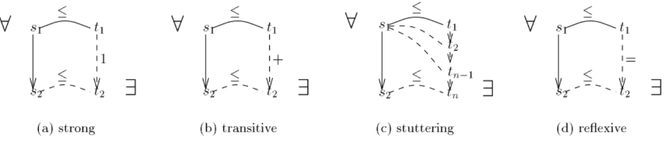
Further results need slightly restricted notions of compatibility: transitive compatibility and stuttering compatibility.

4.2 Transitive and stuttering compatibility

Denition 4.4. A WSTS

has strong compatibility if for all s

t

and transition s

s

, there exists a transition t

t

with s

t

.

S

has transitive compatibility if for all s

t

and transition s

s

, there exists a non-

empty sequence t

t

t n with s

t n .

S

has stuttering compatibility if for all s

t

and transition s

s

, there exists a non- empty sequence t

t

t n with s

t n and s

t i for all i < n .

S

has reexive compatibility if for all s

t

and transition s

s

, either s

t

or there exists a transition t

t

with s

t

.

See Figure 2 for a diagrammatic presentation of these renements of compatibility.

PSfrag replacements

8

9

s

s

t

t

t

t n

t n

1

(a)strong

PSfrag replacements

8

9

s

s

t

t

t

t n

t n

1

+

(b)transitive

PSfrag replacements

8

9

s

s

t

t

t

t n

t n

1

+

(c)stuttering

PSfrag replacements

8

9

s

s

t

t

t

t n

t n

+ 1 =

(d)reexive

Figure 2: Transitive and stuttering compatibility

Strong compatibility (also called \1-1 compatibility") is inspired from classical strong simu- lation and the other forms of compatibility we use are more general than this.

Reexive compatibility is strong compatibility for

.

Transitive compatibility is slightly less general than the \reexive-and-transitive" compat- ibility we used in Def. 2.5. Finkel's notion of \3-structured systems" [Fin90] uses transitive compatibility in a framework where labels of transitions are taken into account.

Stuttering compatibility, introduced in [KS97a], is less general than transitive compatibility.

The name comes from \stuttering" [BCG88] (also \branching" [GW89]) bisimulation. Both are more general than strong compatibility.

In practice, the strong, \1-1", notion used by Abdulla et al. is much more limited than appears at rst sight. Clearly, their motivation was the decidability of simulation with a nite- state system. Unfortunately most examples do not have strong compatibility, so that for e.g.

Lossy Channel Systems they have to modify the semantics of the model.

More generally, when

=

S;

;

is a WSTS, then

=

S;

;

has strong, \1-1", compatibility, but it is not necessarily a WSTS.

is in general not nitely branching. Worse, when eectiveness issues are taken into account,

needs not have eective Succ or pred-basis even when

has. Finally, the inevitability properties investigated in [ACJY96] do not translate from

(or

) to

.

4.3 Termination

Assume

is a WSTS with transitive compatibility.

Proposition 4.5.

has a non-terminating computation starting from s i FRT ( s ) contains a subsumed node.

Proof. (

): Consider a non-terminating computation. A nite prex labels a path in FRT ( s )

(Lemma 4.3). The last node of this path is a leaf node, not labeled with a terminal state, hence

a subsumed node.

(

): If n

: t

is the leaf node subsumed by n

: t

, we have s

t

t

with t

t

. Transitive compatibility allows to infer the existence of some t

t

with t

t

. Repeating this reasoning, we build an innite computation starting from s .

Hence we have

Theorem 4.6. Termination is decidable for WSTS's with (1) transitive compatibility, (2) de- cidable

, and (3) eective Succ .

4.4 Eventuality properties

Assume

is a WSTS with stuttering compatibility.

Proposition 4.7. [KS97a] Assume I is upward-closed. There exists a computation starting from s where all states are in I i FRT ( s ) has a maximal path where all nodes are labeled with states in I .

Proof. (

): Use Lemma 4.3.

(

): Assume that n

: t

;::: ;n k : t k is a maximal path in FRT ( s ) with all labels in I . If n k is a live node, then t

t

t k is a computation and we are done. If n k is a dead node, then we display an innite computation ( s =) s

s

where all states are greater (w.r.t.

) than one of the t i 's, and thus belong to I .

We dene the s i 's inductively, starting from s

= s (= t

). Assume we have already built s

;::: ;s n . We have s n

t i for some i

k . There are two cases:

i < k : then t i

t i

. Because of stuttering compatibility, there exists a sequence s n

!

s m ( m > n ) with s n ;::: ;s m

t i and s m

t i

. We use them to lengthen our sequence up to s m .

i = k : then, because n k is dead, t j

t k for some j < k . Thus t j

s n , so that we are back to the previus case and can lengthen our sequence.

Now we can generalize a Theorem from [ACJY96].

The control-state maintainability problem is to decide, given an initial state s and a nite set Q =

t

;::: ;t m

of states, whether there exists a computation starting from s where all states cover one of the t i 's. The dual problem, called the inevitability problem, is to decide whether all computations starting from s eventually visit a state not covering one of the t i 's.

Concrete examples abound. See Part II. E.g. for Petri nets, we can ask whether a given place will inevitably be emptied.

Theorem 4.8. The control-state maintainability problem and the inevitability problem are de-

cidable for WSTS's with (1) stuttering compatibility,(2) decidable

, and (3) eective Succ .

Proof. Thanks to Proposition 4.7, the control-state maintainability problem reduces to checking

whether FRT ( s ) has a maximal path with all labels in

Q .

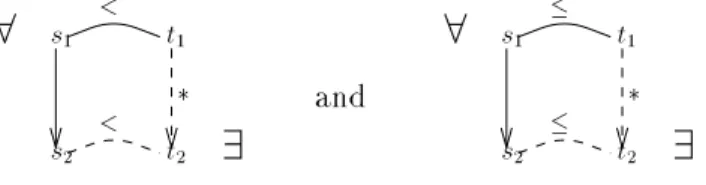
4.5 Strict compatibility

Finkel [Fin90] also considered WSTS's with strict compatibility. Strict compatibility is a stronger form of compatibility.

Denition 4.9. A WSTS

has strict compatibility if for all s

< t

and transition s

s

, there exists a sequence t

t

with s

< t

.

Note that strict compatibility already requires normal non-strict compatibility by assuming that

is a WSTS. When

is a partial ordering, strict compatibility alone entails non-strict compatibility. We adopted the more general denition for situations where

is a quasi-ordering.

Strict compatibility means that from strictly larger states it is possible to reach strictly larger states. See Figure 3 for a diagrammatic presentation. Of course the concept can be combined

PSfrag replacements

8

9

s

s

t

t

t

t

t

8

9

s

s

t

t

<

<

and

PSfrag replacements

8

9

s

s

t

t

t

t

t

8

9

s

s

t

t

< <

Figure 3: Strict compatibility with transitive, stuttering, ::: compatibility.

When we have strict compatibility, the Finite Reachability Tree contains information per- taining to the niteness of the number of reachable states. Assume that

=

S;

;

is a WSTS with strict transitive compatibility. Further, assume that

is a partial ordering (not a quasi-ordering).

Proposition 4.10. For any s

S , Succ

( s ) is innite i FRT ( s ) contains a leaf node n : t subsumed by an ancestor n

: t

with t

< t .

Proof. (

:) If n : t is subsumed by n

: t

then

admits an innite computation s

t

t

t

::: with t i < t i

for all i = 0 ; 1 ; 2 ;::: . This computation is easily built inductively by picking t

= t and t

= t

. Then, strict transitive compatibility allows us to deduce, from t i

t i and t i

< t i the existence of a t i

t i

with t i < t i

. Then the t i 's are all distinct and Succ

( s ) is innite.

(

:) Assume Succ

( s ) is innite. We rst show that there exists a computation starting from s without any loop, i.e. where all states are distinct. For this, we cannot simply remove loops from an innite computation as this may well result into a nite prex only. So we rather consider the (nitely branching) tree of all prexes of computations. Now prune this tree by removing all prexes with a loop. Because any reachable state can be reached without a loop, the pruned tree still contains an innite number of prexes. Now Konig's lemma gives us an innite computation with no loop.

We now apply Lemma 4.3 to this computation: this provides a node n : t subsumed by n

: t

with t

= t

. Hence t

< t because

is a partial ordering.

Now we can generalize a Theorem from [Fin90].

The boundedness problem is to decide, given a TS

and some state s

S , whether Succ

( s ),

the \set of reachable states", is nite.

Theorem 4.11. The boundedness problem is decidable for WSTS's with (1) strict transitive compatibility, (2) a decidable

which is a partial ordering, and (3) computable Succ .

Proof. We can apply Prop. 4.10 so that it is enough to build FRT ( s ) and inspect it for a subsumed node with strict subsumption. This can be done when Succ and

are eective.

5 Downward-WSTS's

There also exists a notion of downward-WSTS, rst introduced in [KS97a] for the RPPS model.

We generalize it to

Denition 5.1. A downward-WSTS is a TS

=

S;

;

equipped with a qo

S

S between states such that the two following conditions hold:

(1) well-quasi-ordering:

is a wqo, and

(2) downward-compatibility:

is downward-compatible with

, i.e. for all s

t

and transition s

s

, there exists a sequence t

t

such that s

t

.

See Figure 4 for a diagrammatic presentation of downward-compatibility. Downward-WSTS's PSfrag replacements

8

9

s

s

t

t

t

t n

t n

8

9

s

s

t

t

Figure 4: Downward compatibility

have been less investigated, partly because only a few recent models give rise naturally to WSTS's with downward-compatibility. In Part II, we shall see several examples.

Assume

=

S;

;

is a downward-WSTS with reexive compatibility and K;K

are two sets of states.

Lemma 5.2.

K

K

implies

Succ

( K )

Succ

( K

).

Proof. (Recall that Succ

( K ) is K

Succ ( K ).) Assume s

Succ

( K ). Then there exist s

K and t

with s

t

s . Because

K

K

, there is a s

K

with s

s

. Because

S

is a downward-WSTS with reexive compatibility, there exists a s

t

with t

t

. Hence t

s . Now t

Succ

( K

) entails s

Succ

( K

).

Now assume s

S and dene a sequence K

;K

;::: of sets with K

=

s

, and K n

= K n

Succ ( K n ). Let m be the rst index such that

K m =

K m

. Such an m must exist by Lemma 2.4.

Lemma 5.3.

K m =

_i

K i =

Succ

( s ).

Proof. The rst equality is a direct consequence of Lemma 5.2, the second follows from the

denition of the K i 's.

Proposition 5.4. If

is a downward-WSTS with (1) reexive compatibility, (2) eective Succ , and (3) decidable

, then it is possible to compute a nite basis of

Succ

( s ) for any s

S . Proof. We proceed as with Prop. 3.5, The sequence K

;K

;::: can be constructed eectively (each K i is nite and Succ is eective). The index m can be computed by computability of

. Finally, K m is a computable nite basis of

Succ

( s ).

The sub-covering problem is to decide, given two states s and t , whether starting from s it is possible to be covered by t , i.e. to reach a state t

t .

Theorem 5.5. The sub-covering problem is decidable for downward-WSTS's with (1) reexive compatibility, (2) eective Succ and (3) decidable

.

Proof. Thanks to Proposition 5.4, one can compute K , a nite basis of

Succ

( s ). It is possible to be covered by t starting from s i t

K . By decidability of

, it is possible to check whether t

K .

Part II

The ubiquity of WSTS's

In this second part we review several fundamental computational models and discover instances of WSTS's in these frameworks.

In general, all the well-structured systems we mention enjoy the eectiveness requirements assumed e.g. by Theorems 3.6, 4.6, 4.8 and 5.5. We will not state this explicitly every time. In fact, we mainly state the few exceptions, all of them occurring when we use a non-trivial

for which decidability is lost.

6 The well-structure of Petri nets

Petri nets are a well-known model of concurrent systems. See [Pet81, Rei85] for a general presentation.

Formally a net N =

P N ;T N ;F N

has a nite set P N of places, a nite set T N of transitions (with P N

T N =

) and a ow matrix F N : ( P N

T N

T N

P N )

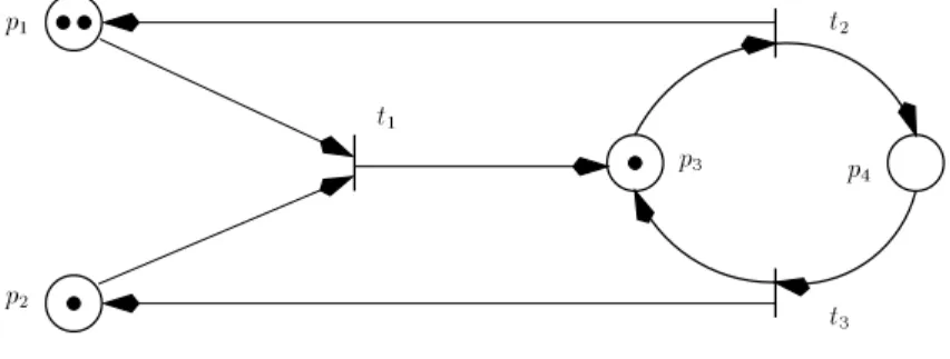
. Figure 5 contains an example net. The congurations of a net N are markings, which can be seen as P N -indexed

PSfrag replacements

8

9

s

s

t

t

t

t

t

p1

p

2

p

3

p

4 t

1

t2

t

3

Figure 5: A Petri net

vectors of non-negative integers, or as multisets of places. The marking M

depicted in Figure 5 is denoted

p

;p

;p

;p

or p

p

p

.

The simplest ordering between markings is inclusion: M

M

when M ( p )

M

( p ) for every place. That it is a wqo is known as Dickson's lemma [Dic13].

Petri nets with inhibitory arcs extend the basic model with special \inhibitory" arcs (also called \zero-test" arcs) that forbid (inhibit) the ring of a given transition when a given place is not empty.

Petri nets with transfer arcs [Cia94] extend the basic model with special \transfer" arcs. Here transitions re as usual but their eect is richer: the transfer arcs say whether the full content of some place must be transfered (added) to some other place.

Petri nets with reset arcs [Cia94] extend the basic model with special \reset arcs" telling how the ring of some transitions resets (empties) some places.

Self-modifying nets [Val78] are Petri nets where the weight on arcs is not a constant anymore.

Rather it is an expression evaluating into a linear combination (with non-negative coecients) of the current contents of the places. Post self-modifying nets are self-modifying nets where the self-modifying extension is only allowed on \post" arcs (arcs from transitions to places).

In all these extensions, reachability becomes undecidable [AK77, Val78]. However

Theorem 6.1. Using the inclusion ordering,

1. Petri nets are WSTS's with strong strict compatibility,

2. Petri nets with transfer arcs are WSTS's with strong strict compatibility, 3. Petri nets with reset arcs are WSTS's with strong compatibility,

4. post self-modifying nets are WSTS's with strong strict compatibility.

Proof. Obvious.

So that e.g. covering is decidable for them ! Covering is a classical problem in the Petri net eld.

It was known to be decidable since [KM69]. As noted in [ACJY96], a byproduct of Theorem 3.6 is a backward-based algorithm for the covering problem in Petri nets. This also applies to the three extensions (transfer arcs, reset arcs, post self-modifying nets) we mentioned.

As far as we know, all implemented algorithms for this problem use Karp and Miller's cover- ability tree, or the coverability graph, or some such quite complex forward-based method. These methods cannot be generalized to all extensions (e.g. it fails for reset arcs [DFS98]).

Other orderings can turn Petri nets into WSTS's. Assume N =

P;T;F;M

is a marked net (a net with a given initial marking M

). Say a place p

P is unbounded if there are reachable (from M

) markings with an arbitrarily large number of tokens in p . Separate bounded and unbounded places and write P = P b

P nb . Usually, one sees places in P b as \control places"

and places in P nb as \data places" or \counter places".

Now dene the ordering

M

M

M ( p ) = M

( p ) for all p

P b ;

M ( p )

M

( p ) for all p

P nb :

This is a well-ordering over the set of reachable markings. So that, if we associate to a marked net

N;M

a transition system

N;M

containing only the reachable markings we get

Proposition 6.2.

N;M

;

is a WSTS.

This works for all the extensions like post self-modifying nets, etc. we mentioned earlier.

However, the well-ordering is only decidable when we can tell eectively which places of the net are bounded. This can be done for Petri nets and for post self-modifying nets. (For nets with reset arcs and nets with transfer arcs, telling whether a given place p is bounded is not decidable [DFS98]).

The partial bounded reachability problem is, given a marked net N;M

and a marking M , to tell whether from M

it is possible to reach an M

with M

( p ) = M ( p ) for all p

P b .

Theorem 6.3. The partial bounded reachability problem is decidable for Petri nets and post self-modifying nets.

Proof. The partial bounded reachability problem is an instance of the covering problem for

hS

N;M

;

.

The most surprising aspect of this result is the relative simplicity of the algorithmic notions that are involved.

Inhibitory arcs can be handled if we have no synchronization. BPP nets, short for Basic Parallel Processes, are nets where the pre-set of transitions is reduced to a single place [CHM94, Mol96].

Theorem 6.4. With the inclusion ordering, BPP's with inhibitory arcs are downward-WSTS's with reexive compatibility.

Proof. Assume M

M

and M

^t M

. If t is rable in M

then M

^t M

and M

M

. If t is not rable in M

then this cannot be caused by an inhibitory arc because M

M

. Hence M

does not contain pre ( t ). But pre ( t ) is some place p , so that M

p

M

. Now M

is M

p

+ post ( t ) and M

M

.

7 The well-structure of string rewrite systems

A Context-Free Grammar (CFG) is a tuple G =

N G ;T G ;R G

where N G (the non-terminal symbols) and T G (the terminal symbols) are disjoint alphabets and where, writing G for N G

T G , R G

N G

_G is a nite set of production rules of the form X

w . See [ABB97] for details.

Here is an example where we group right-hand sides related to a common left-hand side symbol.

G : S

XY

aSS X

bY

Y

XX

The rules in R G induce a notion of rewrite step: if X

w is in R G then uXv

G uwv for any

u;v . Usually, we are interested in derivation sequences that start from a given, so-called axiom,

non-terminal, and end up with a word in T _G

.

In our previous example, a possible derivation for the terminal word b is

S

G XY

G XXX

G bY XX

G bY X

G bY

G bXX

G bX

G b (1) If instead of focusing on the language generated by G , we emphasize the rewrite steps, then G gives rise to a transition system

G where states are words in

and (1) now is a complete computation of

G , starting from S .

Several natural orderings can be dened between words:

embedding: a word u embeds into a word v (also u is a subword of v ), written u

v , i u can be obtained by erasing letters from v .

left-factor: a word u is a left-factor (also, a prex) of a word v , written u

v , i v is some uw .

Parikh: u

v i a permutation of u is a subword of v .

subset: u

v i any symbol in u is in v .

4

,

are po's while

, and

are qo's. Assuming a nite alphabet,

is a wqo (Higman's Lemma) while

is not. Being larger than

, both

and

are wqo's.

Theorem 7.1. For any CFG G ,

1.

G ;

is a WSTS with strong strict compatibility, 2.

G ;

is a WSTS with strong strict compatibility, 3.

G ;

is a WSTS with strong compatibility.

Proof. Left as an easy exercise.

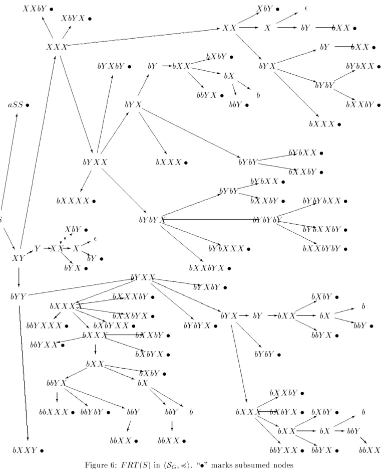
When it comes to applications, the precise choice of which ordering we consider is quite relevant because many decidable properties for WSTS's (e.g. coverability) are expressed in terms of the ordering itself. When a choice is possible, using a larger ordering will often yield less information but more ecient algorithms.

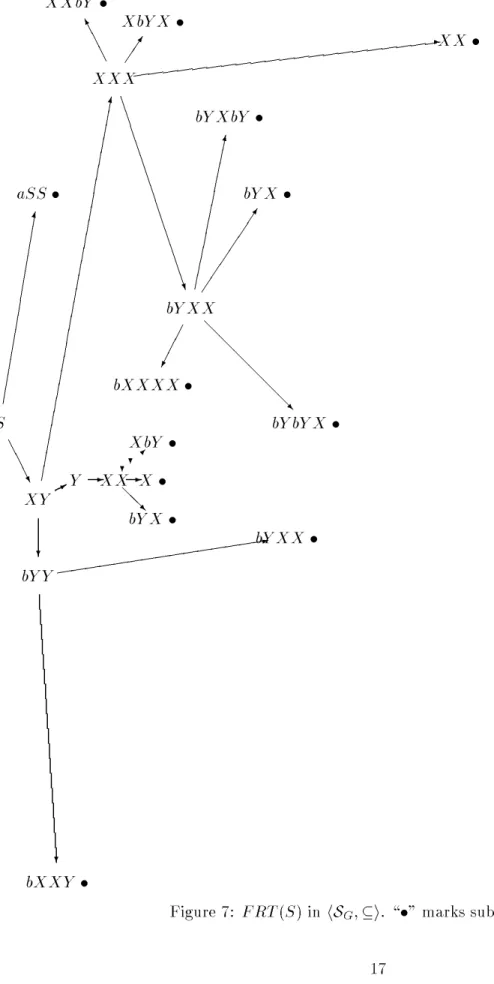
We illustrate this on two dierent well-structured views of context-free grammars. Fig. 6 displays FRT ( S ) for

G ;

. Even though G is quite simple, there FRT ( S ) has 96 nodes.

When we switch to the

G ;

view (see Fig. 7) FRT ( S ) is a subtree of the previous tree and only has 20 nodes.

Of course, there exist many extensions of CFG's which remain partly analyzable. E.g. permu- tative grammars [Mak85] are grammars where context-sensitive permutative rules \ xS

Sx "

are allowed (between any pair of symbols).

Theorem 7.2. For any permutative grammar G ,

G ;

is a downward-WSTS with reexive compatibility.

Proof. Left as an easy exercise.

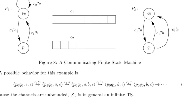
A machine model related to CFG's are stack automata (also pushdown processes). Congu- rations have the form

q;w

where q is a control-state and w

is a stack-content. Quasi- orderings between words lead to quasi-orderings between congurations of a stack automaton.

E.g. with

h

q;w

q

;w

q = q

and w

w

: