A theoretical rationale for flexicurity policies based on education

IHS Economics Series Working Paper 311

March 2015

A theoretical rationale for flexicurity policies based on education

Thomas Davoine

Impressum Author(s):

Thomas Davoine Title:

A theoretical rationale for flexicurity policies based on education ISSN: Unspecified

2015 Institut für Höhere Studien - Institute for Advanced Studies (IHS) Josefstädter Straße 39, A-1080 Wien

E-Mail: o ce@ihs.ac.atffi Web: ww w .ihs.ac. a t

All IHS Working Papers are available online: http://irihs. ihs. ac.at/view/ihs_series/

This paper is available for download without charge at:

https://irihs.ihs.ac.at/id/eprint/3222/

Institut für Höhere Studien - Institute for Advanced Studies │ Department of Economics and Finance

A theoretical rationale for flexicurity policies based on education

Thomas Davoine

1

Institute for Advanced Studies

March 2015

All IHS Working Papers in Economics are available online:

https://www.ihs.ac.at/library/publications/ihs-series/

Economics Series

Working Paper No. 311

A theoretical rationale for flexicurity policies based on education

Thomas Davoine

March 30, 2015

Abstract

The paper provides a theoretical rationale for flexicurity policies, which consist of low employment protection, generous unemployment insurance and active labor market programmes. It analyzes in which conditions flexicurity can be optimal. Low employment protection encourages costly education ef- forts to access high productivity and high innovation sectors, with firms more likely to survive and thus not exposing much their workers to unemployment risk. Activation programmes support the reallocation flow from unproductive to productive firms, helping to reduce unemployment. Low employment pro- tection thus provides incentives for costly self-insurance against unemployment risk through education, mitigating the moral hazard cost of unemployment in- surance and activation programmes. The paper provides realistic numerical illustrations where flexicurity is optimal, and where it is not optimal.

Keywords: flexicurity, unemployment insurance, job protection, active labor market policy, education.

JEL-Classification: J64, J65, J68, J32, H30

1 Introduction

Unemployment remains high in many developed countries. Flexicurity, based on low employment protection, generous unemployment benefits and active labor market policies, has been associated with encouraging signs of unemployment reduction, in Denmark and the Netherlands. Policy analysis present flexicurity as a viable

∗Institute for Advanced Studies, Vienna, Stumpergasse 56, 1060 Vienna, Austria. Contact:

davoine@ihs.ac.at. For useful comments, I am grateful to Christian Keuschnigg, Martin Kolmar, Volker Grossmann and participants in seminars at the Universities of Dortmund, Munich and St.Gallen, and at the L.A. Gerard-Varet conference in Marseille.

option (Bovenberg and Wilthagen, 2009). It is also an example of policy moving ahead of science. This paper provides a theoretical rationale for flexicurity based on education. I show flexicurity can help speed up the job reallocation process due to negative productivity shocks and labor market frictions, encouraging self- insurance through education, balancing low unemployment with high output growth and delivering utilitarian welfare gains.

With one exception, there are no complete theoretical analysis of flexicurity.

There exists a large number of studies which consider a subset of the three policy instruments of flexicurity. For instance, unemployment insurance and employment protection have been jointly considered by Pissarides (2001). Most theoretical anal- ysis of active labor market policies also consider unemployment insurance, including Fredriksson and Holmlund (2006) and Andersen and Svarer (2014).

Using a combination of instruments makes theoretical models more complicated.

To capture interactions and complementarities of the labor market policies and the full potential of flexicurity, one needs however to analyze all three instruments si- multaneously. Andersen and Svarer (2007) remind for instance that low protection and generous unemployment benefits were already in place well before the rise in unemployment in Denmark, following the mid-1970’s oil shock. Only after imple- mentation of active labor market policies did unemployment start to decrease.

Brown, Merkl and Snower (2009) is the only joint analysis of the three policy instruments of flexicurity. They however treat employment protection as a firing cost and miss the potential complementarity effect of firing taxes and unemployment benefits highlighted by Blanchard and Tirole (2008).

This paper builds on Davoine and Keuschnigg (2010) and considers firing taxes (as employment protection), unemployment insurance and active labor market poli- cies, without any preconception of what their optimal level is. Its main contribution is a theoretical rationale for flexicurity. I analytically show that the optimal public policy is flexicurity, under certain conditions related to endogenous education de- cisions. With a plausible calibration, numerical examples where flexicurity is the optimal policy, and where it is not, are provided. A companion paper Davoine and Keuschnigg (2015) performs an analysis to investigate the benefits of coupling flexicurity with redistribution or re-employment wage subsidies.

I use a model where low productivity firms may have to downsize or shut down and fire workers. To be hired by high productivity and innovative firms, which reduces exposure to unemployment risk, households need to educate, at a cost.

Firing, job search and education decisions are endogenous. I follow Blanchard and Tirole (2008) to model firing decisions, Hopenhayn and Nicolini (1997) as well as Chetty (2008) for job search decisions and Heathcote, Storesletten and Violante (2010) for education decisions.

Government offers unemployment benefits to the unemployed, financed by labor

income taxes and, if any, firing taxes. Unemployed are enrolled in active labor

market programmes, which help them retrain and find jobs, but are time consuming

and reduce benefits of home production. Each policy instrument comes with a

trade-off. High unemployment insurance increases the welfare of the unemployed

but reduces the incentive to search for a job. High firing taxes reduces the inflow

into unemployment but reduces the incentive to educate and join safer, innovative and productive firms. Large active labor market programmes speed up reallocation but are costly, both for the unemployed and for the state.

The paper shows that flexicurity - low firing taxes, high unemployment benefits and large active labor market programmes - is optimal under conditions related to education and job search behavior. In particular, optimal unemployment insurance and firing taxes are substitutes if education efforts decrease with firing taxes and other conditions are satisfied. Intuitively, low firing taxes reduce employment pro- tection in risky, low-productivity but free access firms while they increase education efforts and access into safer, innovative and productive firms. A marginal decrease of employment protection thus allows for a marginal increase of unemployment benefits, as more households join safer firms. Flexicurity in this case encourages self-insurance against unemployment risk through education, mitigating the moral hazard cost of public unemployment insurance.

The next section presents the model. Section 3 contains analytical results. A numerical illustration is provided in section 4 and a conclusion in section 5.

2 Model

Policy instruments which are part of flexicurity impact both firms and household decisions. Consistent with empirical evidence, employment protection influences firing decisions by firms (see for instance Boeri and Jimeno, 2005) while unemploy- ment benefits and active labor market policy impacts the effort and the success of job search (see respectively Krueger and Meyer, 2002; Card, Kluve and Weber, 2010).

Endogenous firm and household decisions responding to the three flexicurity policy instruments create modelling complexity. To maintain tractability and obtain analytical results, I keep the model simple in some dimensions. In particular, the model is static, labor supply is inelastic and I use some reduced-form specifications.

The impact of these simplifications is discussed in section 5.

Firms and sectors Workers affected by firms closures need to seek jobs in sur- viving firms. To analyze worker reallocation flows and their dependence on policy, I separate firms in two sectors. In the first sector, I regroup firms which innovate little, have a low productivity and face a high risk of closure. The second sector consist of firms which innovate, install new production process, are more produc- tive and more likely to survive. The precise definition and characteristics of sectors follows.

All firms employ exactly one worker and produce the same good, which I take as numeraire

. In a static framework with inelastic labor supply normalized to unity, production is Ricardian.

Innovation allows firms from the second sector to produce at a cheaper cost. For

1Extending the model to multiple goods, one could also integrate a simple form of Schum- peterian creative destruction (Schumpeter, 1942; Aghion and Howitt, 1994). Sector 1 firms which do not innovate may see their market stolen by sector 2 firms, which offer new products. If this happens to a sector 1 firm, it needs to close down and sends its workers into unemployment.

simplicity, I assume that firms in the second sector always survive and that they are equal (that is, there is a representative firm). While there is uncertainty in the first sector, there is none in the second sector.

Uncertainty and firm behavior in the first sector is taken from Blanchard and Tirole (2008). There are four phases in the life of a sector 1 firm. First, an investor decides to create a firm

. Second, the firm hires one worker at an agreed wage.

Assuming free entry, expected profits are driven down to zero, so that the wage will be equal in all firms, w

. Third, the firm learns about the level of competition from innovative firms. Relative to the representative firm in sector 2, it is given a productivity which is high or low. The relative productivity shock x ∈ [0, ∞) is drawn from a given distribution with density g (x). Four, the firm decides to operate or close down. If its relative productivity x is high, it can survive and expects a profit x − w

. If it is too low, it will make no profit. The firm has to pay a tax t

if it decides to downsize, close down and fire the worker

.

The firm decides to operate if and only if x −w

≥ −t

. The level x

≡ w

−t

is the cut-off productivity above which the firm continues to operate and below which it closes down. Clearly policy influences firms decisions: the higher the firing tax, the lower the rate of firm exits and the flow of workers into unemployment. The tax thus can be used as employment protection (EP). Given these definitions, the separation rate is

s = s (x

) = ˆ

0

g (x) dx. (1)

I assume that firm owners are risk-neutral and operate a portfolio of firms

. Then, owners start with several firms and pay firing taxes for these firms which need to close down with the profit they make from surviving firms. Taking into account policy on firing and the level of competition, expected profits upon entry are

π = ˆ

x1

(x − w

) g (x) dx − st

= (1 − s) (x

− w

) − st

> 0, (2)

where x

≡ ´

x1

xg (x) dx .

(1 − s) is the average productivity of surviving firms.

Free entry drives expected profits to zero. Given the relative productivity distri- bution g (x) and firing taxes t

, this pins down the sector 1 wage w

. Higher firing taxes thus not only reduces the separation rate s but also the average productivity level x

and thus the equilibrium wage w

. Sector 1 workers thus both lose and win from higher firing taxes.

Firms in sector 2 are innovative and safe. They are identical and offer an exogenously given wage w

to workers. I assume that sector 2 is big enough to ensure a level of competition due to innovation such that (via the sector 1 productivity

2In reality, investors often have to pay sunk investment costs. I add these costs in the numerical illustration.

3Notice periods, firing rules and severance payments are more common than firing taxes as a mean of employment protection in OECD countries. Even though not widespread, firing taxes remain a realistic policy instrument. The US for instance uses firing taxes (via the so-called experience rating system for financing unemployment insurance). Blanchard and Tirole (2008) identify an optimal complementarity of firing taxes and unemployment insurance, which can play an important role in the optimality (or not) of flexicurity. One can also think of severance payments as a bundled firing tax with unemployment insurance.

4Alternatively, we could assume that there is a financial intermediation sector with perfect competition and which is costless.

distribution g)

w

< w

. (3)

Intuitively, it makes sense that the innovating sector has higher productivity and thus can offer higher wages. With free entry of firms into sector 2 and no uncertainty, there are no profits so the output of each firm equals the wage w

. While entry is free for firms, it is costly for workers: development and operation of high productivity processes depends on innovation performed by skilled workers, who went through a costly education. Workers entry into sectors will be presented below.

Labor market The labor market is imperfect, due to relocation costs, skill mis- match, search and other frictions. Unproductive firms from sector 1 fire their work- ers, who become unemployed. During unemployment, workers engage in home production

h, retrain to acquire the skills needed for sector 2 and search for a job in that sector. If the retraining and search are successful, they leave unemployment.

Otherwise, they remain unemployed.

As Chetty (2008), I borrow from Hopenhayn and Nicolini (1997) the modelling of search effort decisions, based on reduced-form specifications. Let e ∈ [0, 1] be the individual retraining and search efforts by unemployed workers

. By a suitable nor- malization and the law of large numbers, e also represents the probability of finding a job in sector 2 after separation from sector 1. The reduced form specification ζ (e) captures search effort costs, in utility terms. I assume that utility costs increase with effort and that finding a job becomes increasingly difficult with effort, ζ

> 0 and ζ

> 0. A rapidly increasing function ζ (e) also captures the difficulty of find- ing a job due to adverse labor market conditions, such as job rationing (Michaillat, 2012).

Government provides unemployment insurance (UI) benefits b to unemployed workers and enrolls them in active labor market programmes (ALMP). These pro- grammes include job search assistance, retraining courses and can also include mon- itoring and sanctions (for a recent overview, see Card, Kluve and Weber, 2010).

Whether or not they include monitoring and sanctions, participation in these pro- grammes takes time, reducing the output or benefit unemployed workers derive from home production

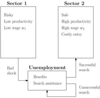
. Figure 1 provides an overview of the labor market and reallocation flows.

Let m ≥ 0 be the amount of active labor market programmes provided to unemployed workers and let the reduced forms ψ (m) and φ (m) capture the two essential dimensions of these programmes. The first dimension reduces the output or benefit from home production to ψ (m) h, with ψ (m) ∈ [0, 1], ψ (0) = 1, and ψ

< 0: the larger the provision of activation measures, the lower the time for or the enjoyment of home production. Monitoring and sanctions can also be part of these measures. The second dimension increases the likelihood of finding a job,

5Aguiar, Hurst and Karabarbounis (2013), among other empirical studies, find that home production increases during unemployment. For simplicity I assume employed workers do not engage in home production.

6For ease of presentation, I will only refer to search efforts in the continuation.

7In their joint analysis of unemployment insurance and workfare (a special type of active labor market policy), Fredriksson and Holmlund (2006) as well as Andersen and Svarer (2014) also assume that workfare reduce the time available for home production (or leisure).

Sector 1 Sector 2

Risky

Low productivity Low wagew1

Costly entry Safe

High productivity High wagew2

Unemployment

Benefits Search assistance

Successful search

Unsuccessful search Bad

shock

Figure 1: Labor market and reallocation flows

reducing the retraining and search effort to φ (m) ζ (e), with φ (m) ∈ [0, 1], φ (0) = 1, φ

< 0 < φ

: the larger the amount of job search assistance and retraining courses, the more likely to find a job; however, activation programmes become increasingly less efficient.

Households Households are heterogenous in their learning capacity. Education is costly but gives access to the safe, productive and high paying sector 2, consistent with the empirical assortative matching literature (see for instance, Haltiwanger, Lane and Spletzer, 1999). By design, non educated workers are exposed to unem- ployment risk while educated workers are not, consistent with empirical evidence (Nickell, 1979).

Endogenous education decisions are made as in Heathcote, Storesletten and Violante (2010). Households are arranged by their innate learning ability n ∈ [0, 1], uniformly distributed. Education is a costly process requiring efforts, in small amount for high ability households and in large amounts for low ability ones. The effort cost i (n) function captures the utility cost of becoming educated, assumed to be continuous and increasing i

> 0, with i (0) = 0 and i (n) → ∞ for n → 1. Low n indicates low effort cost and high ability. At low ability, efforts cost become very large, reflecting the need of a minimum intellectual capacity for higher education.

The decision to educate or not, equivalently to join sector 2 or sector 1, de- pends on learning ability, the utility value derived from income in each sector and unemployment risk.

Households are risk averse and, in a static environment, consume their income.

With a concave increasing utility function u, labor income tax t

, the utility after joining sector 2 is

V

= u ((1 − t

) w

) . (4)

Given unemployment risk, utility from joining sector 1 is expressed in expected

terms:

V

= (1 − s) · u ((1 − t

) w

) + s · u

, (5) u

= max

e · u ((1 − t

) w

) + (1 − e) · u (ψ (m) h + b) − φ (m) ζ (e) . With probability 1 − s, a worker joining sector 1 is hired by a firm having a large survival chance (drawing a large relative productivity shock), in which case the worker keeps its job, earn wages w

and pay taxes at rate t

. With probability s, the worker is hired by a firm with low productivity and subsequently closing down.

In this case, the worker is fired and enjoys expected utility u

. As seen previously and for a given amount of active labor market programmes m, fired workers spend efforts e at net utility cost φ(m)ζ (e) to retrain and find a job in sector 2. By the law of large number and via renormalization, e also represents the probability of finding a job. If unsuccessful, fired workers remain unemployed, consuming welfare benefits b and home production ψ (m) h, net of activation measures

.

The endogenous allocation of workers to sector takes place as follows. Individ- uals born with high learning ability (low n) will spent (low) efforts i (n) to educate and join the safe and high paying sector 2. Individuals with low ability find educa- tion efforts too large, will not educate and join the risky and low paying sector 1.

In between, there is a household with ability N who is indifferent between the two sectors,

V

= V

− i(N ). (6)

Households with ability n ≤ N will educate and join sector 2. Those with ability n > N will not educate and join sector 1. With a population size normalized to one and recalling that ability n is uniformly distributed, N also measures the entry rate into the costly

but safe and high paying sector 2.

Aggregates Taking separation and reallocation flows into account, households can end up in one of three states: employed in sector 1, employed in sector 2 or unemployed. The respective size of each group is given by

L

= (1 − s) (1 − N ) L

= N + es (1 − N) δ = (1 − e) s (1 − N ) , (7) with δ the unemployment rate. Since each firm hires exactly one worker, the final number of firms in each sector is given by L

and L

. Given the Ricardian pro- duction technology, inelastic labor supply and sector 1 average productivity x

, the total production in each sector and gross domestic product are respectively

X

= (1 − s) x

(1 − N ) X

= w

L

X = X

+ X

(8)

8I assume that the levelbof unemployment benefits is non-degenerate, in the sense that being hit by the unemployment shock is worse than not being hit by the shock, u((1−tl)w1) > u^e. An alternative assumption to prevent spontaneous quits from sector 1 workers is that the search effort costsζare large and active labor market programmesφquickly inefficient.

9Note that entry costs into sector 2 can include other costs than education. For instance, they can represent foregone consumption opportunities in a static model (or liquidity constraints in a dynamic model) or restrictions to higher education (such as numerus clausus). For ease of presentation, I continue the presentation with education costs only, but may refer to entry costs in general.

Government To each unemployed worker, the government provides unemploy- ment insurance benefits b and active labor market programmes in quantity m at unit cost k. The government also has own consumption C. It finances expenditures with labor income taxes at rate t

and firing taxes t

. Ruling out government debt by imposing balance in the budget, the net fiscal balance satisfies

T = t

w

L

+ t

w

L

+ t

s (1 − N ) − [δb + mks (1 − N ) + C] = 0 (9)

3 Theoretical analysis

I start by characterizing firms and households behavior and continue with properties of optimal policy. I finish with the main theoretical result, an identification of flexicurity as optimal, or non-optimal, policy.

To obtain compact formulas, I use the notation u

≡ u ((1 − t

) w

), u

≡ u (ψ(m)h + b) as well as u

≡ u ((1 − t

) w

). The index refers to the final state of the worker, employed in sector 1, engaged in home production while unemployed or employed in sector 2. Further notations will be presented in due time.

3.1 Behavior

Firms behavior The only uncertainty lies in sector 1: low productivity firms are threatened by competition and may decide to fire their workers and close down if their relative productivity level is too low. High productivity firms, in sector 2, face no uncertainty. The only decision by firms is firing, in sector 1.

Under free entry expected profit π is driven to zero, defining the firing be- havior and pinning down the equilibrium wage w

. Using (1) and (2), the sen- sitivity of profit to firing and the cut-off productivity x

are given by dπ/dx

=

− (x

− w

+ t

) g (x

). By the envelope theorem, dπ/dw

= − (1 − s) and dπ/dt

=

−s. Combining and using the chain rule, the policy sensitivity of the equilibrium wage w

and the separation rate s, characterizing firing decisions, are given by

dw

dt

= − s

1 − s , ds

dt

= −σs, σ ≡ g (x

)

(1 − s) s . (10) As expected, a larger firing tax t

reduces the separate rate. Because more unpro- ductive jobs are kept alive with a larger tax, the average productivity in sector 1 is lower. Free entry and zero expected profits then requires a lower equilibrium wage.

Household behavior In our static and inelastic labor supply framework, house- holds take only two decisions: education and, if unemployed, search efforts. I characterize search efforts decisions first.

If unemployed, workers choose search efforts to maximize the likelihood of find- ing a job in the safe sector, taking into account the effort cost of searching, the support m from active labor market programmes and the value of unemployment benefits b. Formally, they choose effort e to maximize expected utility u

, defined in (5). Differentiating and equating to zero, job search efforts satisfy

φ (m) ζ

(e) = u ((1 − t

) w

) − u (ψ (m) h + b) (11)

Total differentiation then characterizes search response to policy changes,

de = −ε

w

e · dt

− ε

(1 − e) · db + ε

· dm, (12) where

ε

≡ u

eφζ

> 0, ε

≡ u

(1 − e) φζ

> 0, ε

≡ − φ

ζ

+ u

ψ

h φζ

> 0.

Elasticity parameters ε

capture the strength of the search response to policy changes. For instance, when unemployment benefits b are small and increased, by concavity of the utility function u, the elasticity ε

is large and the search response e drops much.

I continue with education decisions, characterized by the fraction N of house- holds who choose to become educated.

The fraction N is defined by i(N ) = V

− V

, as per (6). Total differentiation of (5) provides the variation of expected utility V

with policy changes,

du

= −u

w

edt

+ u

(1 − e) db +

(1 − e) u

ψ

h − φ

ζ dm, dV

= u

(1 − e) sdb − u

w

esdt

+

(1 − e) u

ψ

h − φ

ζ sdm

−u

w

(1 − s) dt

− (1 − t

− ∇σ) u

sdt

,

with the notational shortcut ∇ ≡ (u

− u

) /u

, positive by assumption on labor market policy. An increase in unemployment benefits db > 0 increases the expected utility u

of unemployed workers and thus the ex-ante utility V

of workers who choose the risky sector 1. Active labor market programmes have ambiguous effects:

more activation measures dm > 0 increases ex-ante utility V

as long as the job search assistance component −φ

ζ > 0 dominates the reduction of home production benefits component (1 − e) u

ψ

h < 0. Employment protection also has ambiguous effects. A higher firing tax dt

> 0 reduces firing by ds = −σsdt

, thus increasing expected utility by (u

− u

) (−ds) = ∇u

(−ds). It also reduces the wage rate by dw

= −

dt

. As this event takes place with ex-ante probability 1 − s, expected utility is reduced by (1 − s) u

(1 − t

) dw

.

Total differentiation of i(N ) = V

− V

leads to the following response equation for education decisions,

dN = η

w

(1 − s) (1 − N ) dt

− η

w

(1 − es) dt

(13)

−η

(1 − e) s (1 − N ) db + η

s (1 − N ) dt

− η

s (1 − N ) dm, where

η

≡ u

(1 − N ) i

> 0, η

≡ u

i

> 0, η

≡ u

(1 − N ) i

> 0 η

≡ (1 − t

− ∇σ) η

, η

≡ (1 − e) u

ψ

h − φ

ζ

(1 − N ) i

.

Higher unemployment benefits db > 0 reduce the loss due to sector 1 separation so decreases education efforts. The signs of η

and η

may be positive or negative:

additional employment protection t

and active labor market programmes m have

ambiguous effects, mirroring the dV

variations discussed above. In particular, education efforts are increased with activation programmes (η

< 0) if and only if the home production benefit reduction effect ((1 − e) u

ψ

h < 0) dominates the assistance effect (−φ

ζ > 0) for workers losing their sector 1 jobs.

Fiscal impacts Labor markets and the fiscal balance (9) are impacted by edu- cation decisions dN, firing (separation) decisions ds and job search decisions de.

Effective tax rates τ

, τ

and τ

for each margin capture the influence of behavior on net tax revenue,

dT = (N + es (1 − N )) w

dt

+ (1 − s) (1 − N ) · w

dt

+ (1 − t

) s (1 − N ) · dt

− (1 − e) s (1 − N ) · db − ks (1 − N ) · dm +τ

· dN + τ

· (1 − N ) ds + τ

· s (1 − N ) de, where

τ

≡ t

w

+ b, τ

≡ t

+ [et

w

− (1 − e) b] −km −t

w

, τ

≡ t

w

−t

w

−sτ

. τ

represents the effective tax rate on labor market participation, τ

the effective tax rate on firing and τ

the effective tax rate on sector 2 entry. For every un- employed person who finds a new job, there is a fiscal gain τ

, summing up extra revenue t

w

and spared unemployment benefits b. The fiscal impact of job separa- tion τ

sums up the firing tax t

paid by firms and the average tax revenue gain from separation et

w

− t

w

minus the unemployment insurance spending (1 − e) b and active labor market policy spending km. Net tax revenue rises by τ

for each addi- tional person who educates, adding the differences in workers’ tax bills t

w

− t

w

across sectors and removing the average tax revenue τ

from firing, which occurs with probability s.

Using these effective tax rates and substituting (10), (12) and (13) yields a change in net fiscal revenue equal to

dT = L

− τ

η

(1 − es) − τ

ε

s (1 − N ) e w

dt

+ 1 + τ

η

w

(1 − s) (1 − N ) dt

− 1 + τ

η

+ τ

ε

(1 − e) s (1 − N) db + 1 − t

− τ

σ + τ

η

s (1 − N ) dt

− k + τ

η

− τ

ε

s (1 − N ) dm.

(14)

The expression decomposes the effect of public policy and behavioral responses on fiscal revenue. To illustrate, additional active labor market programmes dm in- creases direct expenditures by k·s (1 − N ) dm. Net fiscal revenue is further impacted by education responses, as per (13). There are η

s (1 − N ) dm less households choosing to educate into sector 2, each one reducing by τ

their tax contribution.

On the other hand, the policy supports job finding at rate ε

s (1 − N ) dm, as per (12). Each person who stops claiming benefits and pays taxes adds τ

to govern- ment revenue. The net fiscal cost of active labor market programmes thus sums up to k + τ

η

− τ

ε

s (1 − N ) dm.

3.2 Welfare maximization

This section derives some properties of welfare maximizing policy.

Throughout the paper, I use a utilitarian welfare criteria. Because of free entry, firms make no profit so the social welfare function restricts to welfare V

of entrants in sector i and the cost of entry in sector 2:

V = (1 − N ) · V

+ N · V

− ˆ

0

i (n) dn. (15)

Due to occupational choice (6), a variation of entry N yields dV /dN = −V

+ V

− i (N ) = 0 so welfare variations are dV = (1 − N ) dV

+ N dV

. Substituting expressions from section 3.1,

dV = −u

w

(1 − s) (1 − N ) dt

− u

w

L

dt

+u

(1 − e) s (1 − N ) db +

(1 − e) u

ψ

h − φ

ζ

s (1 − N ) dm (16)

− (1 − t

− ∇σ) u

s (1 − N ) dt

.

The following technical characterization helps analyze optimal policy:

Lemma 1. (optimality conditions): the policy which maximizes utilitarian wel- fare (15) and satisfies the government budget constraint (9) verifies:

dV /db =

u

− 1 + τ

η

+ τ

ε

λ

(1 − e) s (1 − N ) = 0, dV /dt

= −

(1 − t

− ∇σ) u

− 1 − t

− τ

σ + τ

η

λ

s (1 − N ) = 0, dV /dm =

(1 − e) u

ψ

h − φ

ζ − k + τ

η

− τ

ε

λ

s (1 − N ) = 0, where λ is the Lagrange multiplier related to the fiscal constraint.

Proof: see appendix A.

Several properties of optimal policy can be derived from lemma 1, including moral hazard limitations. These are compiled in the following result:

Proposition 1. (optimal policy characteristics): the social welfare maximizing policies have the following properties:

(a) an economy without government and social security policy is not optimal, as unemployment insurance financed with labor taxes increases welfare:

dV

db > 0 when t

= t

= b = m = 0 (b) unemployment insurance is limited:

u

u

= 1 1 + τ

ε

< 1 u

> u

(c) employment protection internalizes firing cost externalities:

t

= t

w

+ [(1 − e) b − t

w

e] + km + ∇

(d) active labor market policies depend on costs and search behavior:

du

/dm

du

/dc

= (1 − e) u

ψ

h − φ

ζ

u

= k − τ

ε

Proof : in part (a), small unemployment benefits db > 0 are financed with taxes dt > 0 to satisfy the budget constraint dT = 0. Using (14) and (16) at t = b = 0 yields dV /dt > 0 and thus dV /db > 0. Parts (b) to (d) are derived from first order conditions in lemma 1. Details are contained in appendix A. QED.

I discuss each part of the proposition in turn.

Start from an economy without government and social security policy (t

= t

= b = m = 0). Part (a) of the proposition shows that a moderate introduction of unemployment insurance (db > 0) financed with a labor income tax (dt > 0) to keep the public budget balanced (dT = 0) is welfare improving. An economy without social security policy is thus not optimal. The result is intuitive: public insurance discourages job search efforts e and increases unemployment δ; however, since tax distortions on search behavior are initially small, the gains from insurance dominate, raising aggregate welfare V .

Part (b) of the proposition illustrates the moral hazard cost of unemployment insurance. The less elastic job search efforts are (the closer to zero the ε-elasticities), the smaller the moral hazard cost, the closer insurance is to full consumption smoothing (u

= u

) between workers in the good state (sector 1 workers not hit by the unemployment shock) and the bad state (sector 1 workers hit by the shock).

Low public finance costs of insurance (low tax revenue losses and unemployment benefits, τ

= t

w

+ b) also push towards full consumption smoothing.

Part (c) of the proposition shows that using a firing tax as employment protec- tion is optimal, as it internalizes negative firing externalities. It plays the same role as in Blanchard and Tirole (2008). Firms who fire a worker create a fiscal external- ity, as there is one person less paying taxes t

w

, one person more who collects an average net benefit (1 − e) b − t

w

e and extra spending km on active labor market policies. Firing also creates a utility loss ∇ = (u

− u

)/u

, expressed in income equivalent terms. All these externalities justify the use of a firing tax.

Note that part (b) and part (c) generalize the optimality results

from Blan- chard and Tirole (2008) to the case of moral hazard. Indeed, in the special case of a single sector 1 (N = 0), no moral hazard (ε

= 0) nor reallocation (e = 0) and no active labor market policies (m = 0), full insurance is optimal (h + b = (1 − t

)w

) and it is financed by firing taxes only (t

= 0).

Finally, part (d) of the proposition shows that active labor market optimal policy also depends on other policies. The leftmost part of the optimality conditions represents the marginal welfare benefit of the policy m, measuring expected welfare utility gains of a fired worker relative to a retained worker. The optimality condition equates the marginal welfare benefit of the policy, on the left, with its marginal cost, on the right. Larger unemployment benefits b increase the participation tax τ

= t

w

+b and thus decrease the net marginal cost of active labor market policy: every persons put back to work thanks to spending m saves costs b and brings revenue

10Specifically, propositions 1 and 2 from Blanchard and Tirole (2008).

t

w

. The larger the unemployment insurance benefits, the more attractive active labor market programmes, typical of flexicurity arrangements. This can explain why flexicurity measures were first introduced by Northern European countries in the 1990’s, who started with high unemployment benefits levels and subsequently introduced large-scale activation measures. In the next subsection, I will perform a formal analysis of the complementarity of all the policy instruments which are part of flexicurity.

3.3 Flexicurity as optimal policy

This section contains the main analytical result. I show that flexicurity is the optimal policy combination under certain circumstances, providing criterias which separate cases where flexicurity is optimal from cases where it is not.

Flexicurity is a combination which exploits policy complementarity. In its most general policy discussion sense and its etymological basis, flexicurity compensates workers for the loss generated by low employment protection (flexibility) with gen- erous insurance and assistance programmes (security): security is provided in ex- change for flexibility.

I therefore analyze complementarity of the three instruments of flexicurity in welfare maximization. Flexicurity corresponds to the case of job protection and unemployment insurance being substitutes; job protection and activation measures being substitutes; while unemployment insurance and activation measures are com- plement.

I provide three preliminary results to characterize policy complementarities, discuss each of them and conclude with a general result

.

Unemployment insurance and active labor market programmes Comple- mentarity of unemployment benefits b and activation measures m is characterized by the following result.

Lemma 2. at the optimum, the sign

d dm

d db V

is equal to the sign of u

ψ

h n

1 −

o

+

n

1 ζ1

φ

+

ζ1

− (1 − e)

u

ψ

h o +

λη

n

s ε

τ

− k

− τ

o

Proof: at the optimum and using lemma 1,

V =

u

− 1 + τ

η

+ τ

ε

λ (1 − e) s (1 − N ) = 0, so

V = (1 − e) s (1 − N )

u

− 1 + τ

η

+ τ

ε

λ

. The sign of

V is thus equal to the sign of

u

− 1 + τ

η

+ τ

ε

λ

,

11For ease of presentation, I provide the results with specifications for certain reduced-forms, namely ζ(e) = ζ0 + (ζ2−ζ0)e^{−ζ1(1−e)} and i(n) = i0 −i1 ·ln (1−n). Results with general specifications and different labor income tax rates in the two sectors are contained in appendix B.

which, after differentiation and substitutions, equals the expression given in the lemma. QED.

The following two observations discuss cases where unemployment insurance and active labor market programmes are complements and when they are substitutes.

Two further cases are discussed in appendix C.

First, when entry is exogenous (dN = η

= 0) and the difficulty of finding a job increases rapidly (ζ

and thus ζ

and ζ

are large), unemployment insurance and active labor market programmes are complements

,

V > 0. The intuition for this result is the following. There is a point where the transition from the bad state (being unemployed) to the good state (finding a job in sector 2) becomes very difficult without further assistance. As activation measures also reduce home production benefit (ψ

< 0), welfare in the bad state can only be maintained when unemployment benefits follow assistance.

Second, consider the case of endogenous entry (η

> 0) with large response to policy variations (η

is large) and net tax revenue depending little on education decisions (τ

is small). Then, if activation measures are cost-effective (k small) or unemployment benefits large (ε

τ

− k > 0, given τ

= t

w

+ b), activation measures and unemployment insurance are complements

,

V > 0. If activa- tion measures are not cost-effective and benefits are small (ε

τ

− k < 0) on the other hand, they are substitutes,

V < 0. The intuition is the following. If unemployment benefits and the entry response are large, many households avoid the costly entry into the safe sector 2: choosing the easy-access but risky sector 1 is attractive, as generous benefits are provided in case of unemployment. The quantity ε

τ

− k represents the marginal gain of one more unit of activation mea- sures, taking tax gains of re-employment into account. When this marginal gain is positive, strong activation measures complements large benefits: putting more people back to work with large assistance helps reduce the aggregate costs of high unemployment benefits.

Unemployment insurance and employment protection Complementarity of optimal unemployment benefits b and firing taxes t

is characterized by:

Lemma 3. at the optimum, sign

d dt

d db V

= sign (η

)

Proof: Similar to the proof of lemma 2,

s

d

db

V has the sign of (1 − e) s (1 − N)

d dts

u

− λτ

η

− λτ

ε

. In the first order condition

V = u

− (1 + τ

η

+τ

ε

λ = 0 in lemma 1, u

represents the marginal gain of one extra unit of unemployment insurance and − 1 + τ

η

+ τ

ε

its marginal public finance cost.

As the former is positive and the latter negative, λ > 0. Since

s

u

=

s

τ

=

d

dts

ε

= 0, the sign of

s

d

db

V equals the sign of

s

−τ

η

, a derivative which, after algebraic manipulation, is shown to equal η

s 1 − t − στ

. From the first

12Indeed, in this case, the sign of _dm^d _db^dV is equal to the sign ofu⁰⁰_hψ⁰h, positive.

13In this case, the sign of _dm^d _db^dV is equal to the sign ofληhs εmτ^E−k

, positive.

and second conditions from lemma 1 follows that 1 − t − τ

σ and 1 − t − ∇σ have the same sign. Then η

= (1 − t − ∇σ) η

and η

> 0 imply that η

s 1 − t − στ

has the same sign as η

sη

. Noting that η

> 0 concludes. QED.

I discuss complementarity of insurance and protection in two noteworthy cases.

First, when entry is exogenous (dN = η

= 0), optimal unemployment insurance and optimal employment protection are independent,

s

d

db

V = 0. The sequenc- ing of events provides the intuition in this case. Households only choose search efforts, which take place after firing. Whether employment protection is high or low, whether the flow into unemployment is low or large, public insurance impacts search efforts of each unemployed the same way. Protection regulates the flow into the bad state (unemployment) and insurance the flow out of the bad state (into re-employment), independently. In contrast, when entry is endogenous, the house- hold choice of sector is jointly impacted by the likelihood of entering the bad state if sector 1 is chosen (regulated by employment protection) and by the comfort in this state (impacted by unemployment insurance).

Second, when entry is endogenous (η

6= 0), unemployment insurance and em- ployment protection are substitutes,

s

d

db

V < 0, if entry in the safe sector increases with lower protection (η

< 0), and vice-versa. I discuss the case where entry into the safe sector increases with lower protection in the risky sector (η

< 0), more intuitive. The idea is to reduce employment protection to attract more people into the costly but safe and productive sector, (partially) curbing inflows into unemploy- ment and allowing higher welfare (through unemployment insurance) for workers remaining in the bad state. Low protection invites increased self-insurance against the unemployment risk through education and reduces the moral hazard cost of high public insurance: a marginal decrease of employment protection allows for a marginal increase of unemployment benefits, as more households join the safe sector

.

Active labor market programmes and employment protection Comple- mentarity of activation measures m and firing taxes t

is characterized by:

Lemma 4. at the optimum, sign

d dt

d dm V

= sign (η

η

)

Proof: following the same steps as in the proof of lemma 3, one has that

s

d dm

V has the sign of η

s 1 − t

− στ

. Noting that 1 − t − τ

σ and 1 − t − ∇σ have the same sign, that η

= (1 − t − ∇σ) η

, that η

> 0 but that η

and η

can be positive or negative concludes. QED.

Two cases are discussed. First, when entry is exogenous (dN = η

= η

= 0), optimal employment protection and activation measures are independent

s

d dm

V =

14Education as self-insurance against the unemployment risk illustrates a less visible channel of employment protection. Often, the literature focuses on job creation and separation effects. In this paper, the self-insurance and separation channels apply, not the job creation one.

0. The intuition is the same as for lemma 3, activation measures impacting house- hold decisions during the same phases as unemployment insurance.

Second, consider the case of endogenous entry where entry in the costly but safe sector increases with low employment protection in the easy-access but risky sector (η

< 0 and η

6= 0). Then optimal employment protection and activation mea- sures are substitutes,

s

d

dm

V < 0, if entry in the safe sector decreases with lower activation (η

> 0), and vice-versa. The intuition is similar to the endogenous entry case in lemma 3, with a variation. When the assistance part of activation measures dominates (φ

< 0 large in absolute value, so η

> 0), these measures gen- erate a similar moral hazard effect as unemployment insurance. Low employment protection encourages higher entry into the costly but safe sector as self-insurance against unemployment risk, reducing the moral hazard cost of activation measures and allowing to provide more assistance. When the sanction part of activation measures dominates (ψ

< 0 large in absolute value, so η

< 0), they have the opposite incentive effects as unemployment insurance. Increase of self-insurance with low protection allows to reduce the discomfort of activation measures, which are reduced.

All three instruments As a corollary

of lemmas 2, 3 and 4, one obtains the following characterization of optimal policy:

Proposition 2. (flexicurity as optimal policy): when the costly entry into the safe sector 2 is negatively related to employment protection (η

< 0), is negatively related to active labor market policies (−η

< 0), active labor market programmes are cost-effective (k is small), net tax revenue is little affected by education choices (τ

is small) and when the difficulty of finding a job increases rapidly (ζ

is large), the welfare maximizing labor market policy is flexicurity, with large unemployment benefits b, large active labor market programmes m and small firing taxes t

:

d dm

d

db V > 0 d dt

d

db V < 0 d dt

d

dm V < 0

I conclude with four observations. First, conditions in proposition 2 are sufficient but not necessary. There can be other cases where the optimal policy is flexicurity

. Discussions of lemmas 2, 3 and 4 provide other such cases.

Second, conditions of proposition 2 are likely to be satisfied for several large European welfare states, but not all. The condition η

< 0 is intuitive, as high employment protection increases the attractiveness of the risky sector. The con- dition η

> 0 is satisfied if the assistance part of activation measures dominates the sanction part, typical in Europe. Those countries which are able to design low

15I take for granted that the combination of high unemployment insurance, large activation mea- sures and low employment protection is the optimal policy, not the combination of low insurance, low activation measures and high protection, which also satisfies the cross-derivative optimality conditions in lemmas 2, 3 and 4. Support is provided by results in section 3.2, showing that the introduction of unemployment insurance increases welfare.

16Specifically, proposition 2 only assembles the first and second cases discussed after lemma 2, the second case after lemma 3 and the second case after lemma 4.

cost activation measures (k small), maintain tax revenue regardless of the education composition of the population (τ

small) and where large persistent unemployment problems indicate rapidly increasing difficulties in finding jobs (ζ

large) fulfill the conditions to benefit from flexicurity policies. Other countries may not.

Third, endogenous entry is key for the result, as the discussion of the self- insurance channel through education in lemmas 3 and 4 makes clear: low protection of jobs in the risky sector invites for more self-insurance against the unemployment risk through costly education, giving access to the safe sector and mitigating the moral hazard cost of public insurance. These results are consistent and complement Andersen and Svarer (2014), where activation measures (workfare) reduce the moral hazard impact of insurance. With exogenous entry, optimal employment protection is independent of both optimal insurance and optimal activation measures, which is far from the idea of policy complementarity at the heart of flexicurity.

Fourth, there is a consistent relationship with the cross-country flexicurity anal- ysis of Algan and Cahuc (2009). Entry decisions in my model are made under expectation of future economic outcomes, including labor income revenue and the likelihood of unemployment. In reality, education decisions are also made for other reasons, such as intellectual satisfaction. When education decisions are solely based on these other reasons, entry becomes exogenous in the model, in which case optimal policy does not exhibit the complementarities of flexicurity. Assume that cultural differences across countries influence education decisions, such that individuals in countries with high civic values feel more responsible for their own economic destiny and thus base more of their education choice on economic prospects than in other countries. Then, entry in high civic values countries is less likely to be exogenous and flexicurity more likely to be optimal. This outcome is consistent with Algan and Cahuc (2009), who find that countries with high civic attitudes are associated with higher unemployment benefits and lower employment protection.

4 Numerical illustration

Numerical examples provide an illustration of the theory. I show that flexicurity is the optimal labor market policy in one case and it is not in another case. Both cases use realistic parameter values, differentiated by the job search elasticity parameter.

Ljungqvist and Sargent (1998) argue that human capital losses through unem- ployment play a role in imperfect labor markets. To reflect their conclusion and deliver more realistic outcomes, I enrich the model. I separate prospects for sector 2 entrants and prospects for sector 1 entrants who were fired, retrained and found a job in sector 2. As the latter suffered from a human capital loss, they are less productive and earn a lower wage, w

< w

. I also assume that sunk investments costs are paid when a firm is created. All theoretical results carry through.

Calibration relies on direct observations or empirical studies. The only excep- tions are parameter values for the active labor market policy functions ψ and φ.

Sensitivity analysis using different values however lead to the same results, with

greater or smaller contrasts. Sensitivity analysis on other parameters also lead to