Approximate and Almost-Exact Aggregation in Dynamic Stochastic Heterogeneous-Agent Models

IHS Economics Series Working Paper 258

October 2010

Approximate and Almost-Exact Aggregation in Dynamic Stochastic Heterogeneous-Agent Models

Michael Reiter

Impressum Author(s):

Michael Reiter Title:

Approximate and Almost-Exact Aggregation in Dynamic Stochastic Heterogeneous- Agent Models

ISSN: Unspecified

2010 Institut für Höhere Studien - Institute for Advanced Studies (IHS) Josefstädter Straße 39, A-1080 Wien

E-Mail: o ce@ihs.ac.atffi Web: ww w .ihs.ac. a t

All IHS Working Papers are available online: http://irihs. ihs. ac.at/view/ihs_series/

This paper is available for download without charge at:

https://irihs.ihs.ac.at/id/eprint/2021/

Approximate and Almost- Exact Aggregation in Dynamic Stochastic Heterogeneous-Agent Models

Michael Reiter

258

Reihe Ökonomie

Economics Series

258 Reihe Ökonomie Economics Series

Approximate and Almost- Exact Aggregation in Dynamic Stochastic Heterogeneous-Agent Models

Michael Reiter October 2010

Institut für Höhere Studien (IHS), Wien

Contact:

Michael Reiter

Department of Economics and Finance Institute for Advanced Studies Stumpergasse 56

1060 Vienna, Austria

: +43/1/599 91-154

email: michael.reiter@ihs.ac.at

Founded in 1963 by two prominent Austrians living in exile – the sociologist Paul F. Lazarsfeld and the economist Oskar Morgenstern – with the financial support from the Ford Foundation, the Austrian Federal Ministry of Education and the City of Vienna, the Institute for Advanced Studies (IHS) is the first institution for postgraduate education and research in economics and the social sciences in Austria. The Economics Series presents research done at the Department of Economics and Finance and aims to share “work in progress” in a timely way before formal publication. As usual, authors bear full responsibility for the content of their contributions.

Das Institut für Höhere Studien (IHS) wurde im Jahr 1963 von zwei prominenten Exilösterreichern – dem Soziologen Paul F. Lazarsfeld und dem Ökonomen Oskar Morgenstern – mit Hilfe der Ford- Stiftung, des Österreichischen Bundesministeriums für Unterricht und der Stadt Wien gegründet und ist somit die erste nachuniversitäre Lehr- und Forschungsstätte für die Sozial- und Wirtschafts- wissenschaften in Österreich. Die Reihe Ökonomie bietet Einblick in die Forschungsarbeit der Abteilung für Ökonomie und Finanzwirtschaft und verfolgt das Ziel, abteilungsinterne Diskussionsbeiträge einer breiteren fachinternen Öffentlichkeit zugänglich zu machen. Die inhaltliche Verantwortung für die veröffentlichten Beiträge liegt bei den Autoren und Autorinnen.

Abstract

The paper presents a new method to solve DSGE models with a great number of heterogeneous agents. Using tools from systems and control theory, it is shown how to reduce the dimension of the state and the policy vector so that the reduced model approximates the original model with high precision. The method is illustrated with a stochastic growth model with incomplete markets similar to Krusell and Smith (1998), and with a model of heterogeneous firms with state-dependent pricing. For versions of those models that are nonlinear in individual variables, but linearized in aggregate variables, approximations with 50 to 200 state variables deliver solutions that are precise up to machine precision. The paper also shows how to reduce the state vector even further, with a very small reduction in precision.

Keywords

Heterogeneous agents, aggregation, model reduction

JEL Classification

C63, C68, E21

Comments

I have benefited from discussions with seminar participants in Istanbul, Barcelona, Vienna, and Zurich.

Support from the Austrian National Bank under grant Jubiläumsfonds 13038 is gratefully

Contents

1 Introduction 1

2 Example 1: The Stochastic Growth Model With

Heterogeneous Agents and Incomplete Markets 3

2.1 Production ... 3

2.2 The Government ... 4

2.3 The Household ... 4

2.4 Finite Approximation of the Model Equations ... 5

2.4.1 Household Productivity, Consumption Function and the Euler Equation ... 5

2.4.2 Wealth Distribution ... 6

2.4.3 The Discrete Model ... 7

2.5 Parameter Values and Functional Forms ... 8

2.5.1 The calibration with i.i.d. shocks ... 8

2.5.2 The calibration with persistent shocks ... 8

2.6 Example 2: An OLG Economy ... 9

3 Exact and Approximate Aggregation in Linear Models 10

3.2 The Reduced State Space Model ... 11

3.2.1 Principal Component Analysis (PCA) ... 13

3.2.2 Conditional Expectations Approach (CEA) ... 13

3.2.3 Balanced Reduction ... 14

3.2.4 Properties of balanced reduction ... 15

3.3 The Aggregation Problem in Linear RE Models ... 16

3.4 Exact and Almost-Exact Aggregation in Linear RE Models ... 17

3.4.1 Exact State Aggregation ... 17

3.4.2 Conditions for exact and almost-exact state aggregation ... 19

3.4.3 Exact policy aggregation ... 20

3.5 Approximate LS Aggregation in Linear RE models ... 22

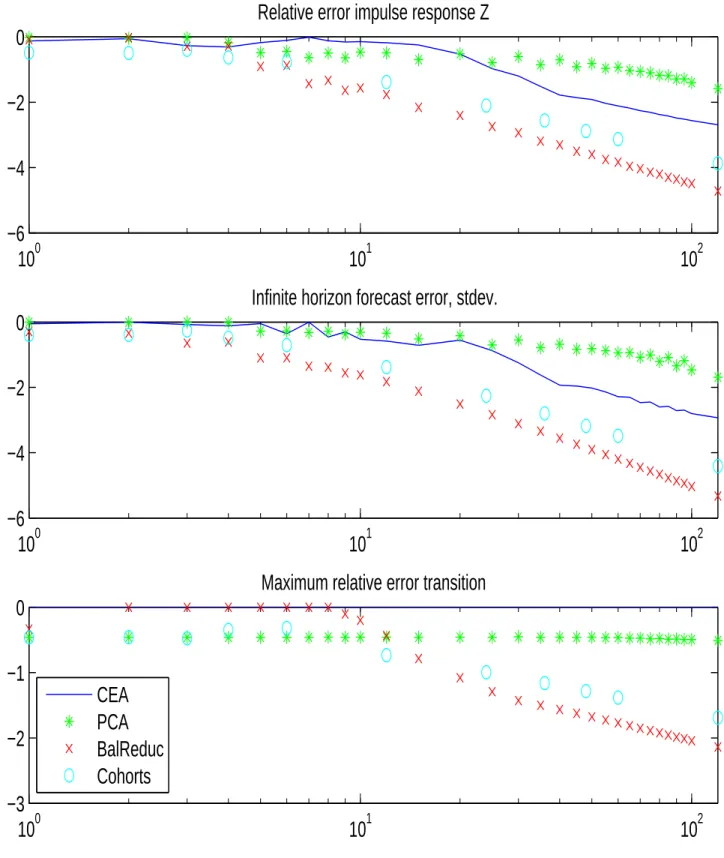
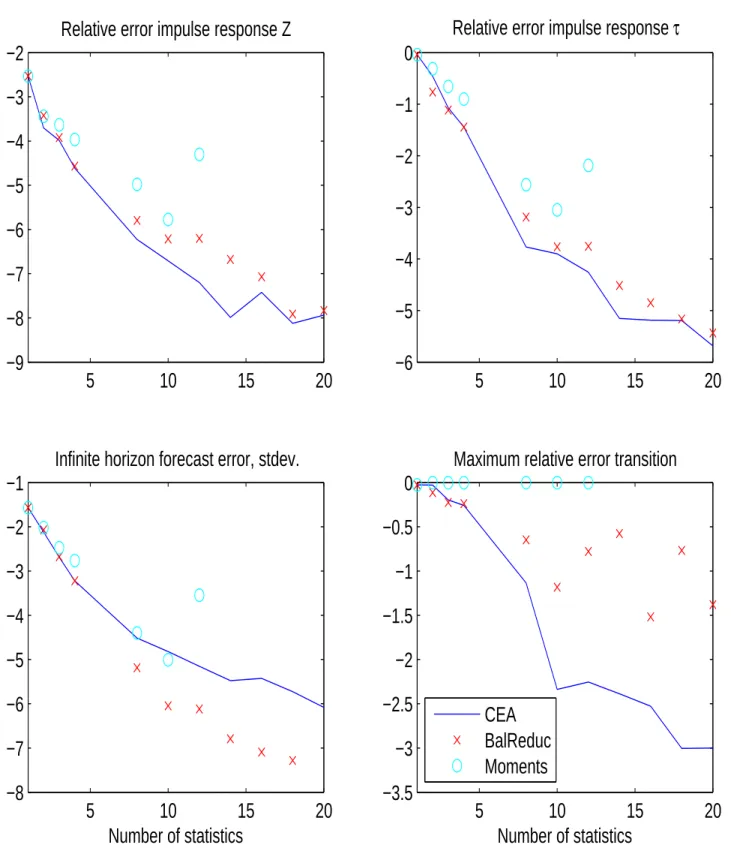
3.6 Evaluating Accuracy ... 23

3.6.1 Types of approximation error ... 23

3.6.2 How to measure the aggregation error ... 24

3.6.3 A variety of accuracy measures ... 24

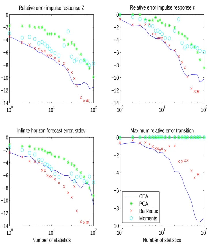
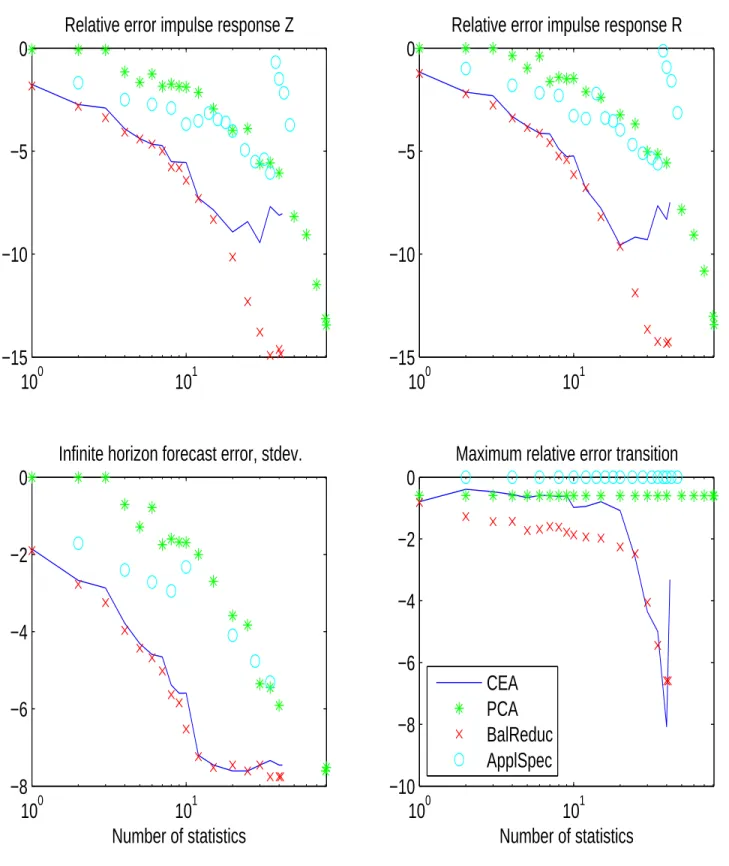
4 Numerical Results 26

4.1 Linearized Krusell/Smith Solution With Few Moment ... 26

4.2 Model Reduction in State Space Form ... 28

4.3 Almost-Exact Aggregation ... 29

4.4 Approximate Aggregation ... 30

4.5 Is Exact Aggregation Possible? ... 31

5 Conclusions 32 A Example 3: A Model of Heterogeneous Firms and State- Dependent Pricing (SDP) 33

A.2 Households ... 34

A.3 Market Clearing and Monetary Policy ... 35

A.4 The Discrete Model ... 36

A.5 Parameter values ... 36

A.6 Choice of grid ... 36

B Asymptotic Estimation of Reduced Model 37

B.2 Stability of Reduced Model ... 37

B.3 Solving Discrete-Time Lyapunov Equations ... 38

B.4 Tikhonov regularization ... 40

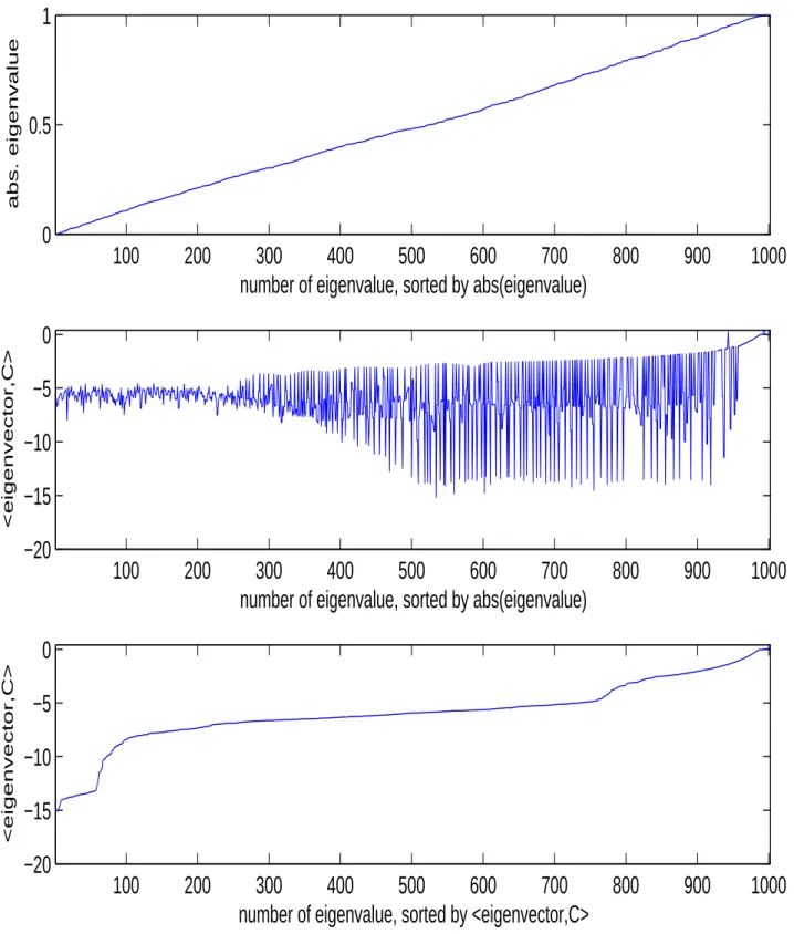
C Almost-exact aggregation 40

C.2 The Numerical Rank of the Observability Matrix ... 41

References 48

1 Introduction

Stochastic general equilibrium models with incomplete markets and a large number (or even a continuum) of heterogeneous agents are now widely used in economics. Except for some special cases, only a numerical solution to these models can be computed. The main computational challenge in solving these models is that, theoretically, the state vector includes the whole cross-sectional distribution of individual state variables of the agents in the economy, which is a high-dimensional or even infinite-dimensional object.

Krusell and Smith (1998) and Den Haan (1996) have shown, in some versions of the stochastic growth model with heterogeneous agents and incomplete markets, that a very good approximate solution can be obtained through approximate aggregation: agents are supposed to base their decision not on the whole state vector of the economy, but only on a very small set of aggregate statistics (such as moments of the cross-sectional distribution of capital). This is a deviation from the assumption of strictly rational expectations, but the available accuracy checks indicate that the resulting approximation is very good (a recent comparison of several solution approaches is cf. Den Haan (2009)). Krusell and Smith (2006) explain and extend this approximate aggregation result.

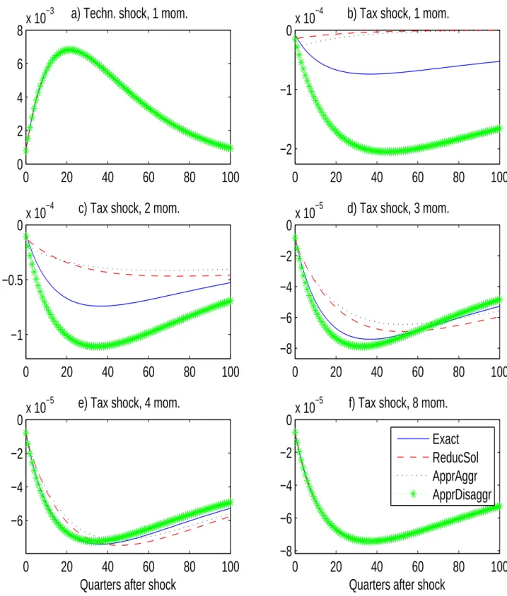
However, we cannot expect such a favorable result to go through in all relevant hetero- geneous agent models. As an example, we will see below that even in the Krusell/Smith model we need approximate solutions with more state variables if we want to study not just technology shocks, but also tax shocks that directly affect the wealth distribution.

Reiter (2009b) has developed a method to handle those cases, using a high-dimensional, non-parametric approximation to the cross-sectional distribution.

The method allows for a nonlinear relationship between individual decisions and individual states, so that it can handle, for example, a consumption function with borrowing constraints. However, the relationship between individual decisions and aggregate states is linearized, which allows to compute a solution with many state variables, in the range of 1000-2000 on a normal PC.

While Krusell and Smith (1998) and most of the subsequent literature use an extreme form of aggregation (only one state variable) to obtain a reasonably precise solution,

Reiter (2009b) goes the opposite way and avoids aggregation by using a high-dimensional state vector. The latter approach has two important limitations. First, a state space of around 1000 state variables appears sufficient to give a precise discrete approximation of a univariate cross-sectional distribution, which is the case of one individual state variable.

However, the constraint on the number of states becomes restrictive if each individual has two or more state variables. Second, linearization in aggregate variables is sufficient for

1Midrigan (2009) shows in a model of state dependent pricing that higher-order moments matter for aggregate dynamics. He solves the model using only one state variable, because those higher-order moments do not vary much. Nevertheless, the precision of the forecasting rule is considerably smaller than in the Krusell/Smith model. To avoid those problems, Costain and N´akov (2008) apply the method of Reiter (2009b) to a similar model.

2Recent innovative approaches such as Preston and Roca (2007) and Haan and Rendahl (2009) can handle a somewhat larger number of variables in the state vector.

many interesting applications, but it is inadequate for others, for example models with asset choice. The question then is whether it is possible to construct aggregate models which give a similarly precise solution, but use a much lower number of state variables, so that higher-order approximations in the aggregate variables can be obtained. Furthermore, for a precise analysis of the properties of the model it is very useful to have a lower-dimensional representation of the solution.

In the present paper I address those issues, by taking a closer look at the aggregation problem in typical dynamic macroeconomic heterogeneous agent models. It turns out that these models do not allow exact aggregation in the theoretical sense, but a substantial reduction in the number of state variables is possible in a way that the approximate solution is still precise basically up to machine precision. Building on results from the systems and control literature on model reduction, I provide a general algorithm to construct such an aggregate model and choose the appropriate state space. The algorithm is independent of the underlying structure of the original state space (whether we have a univariate or a bivariate distribution, etc.). Moreover, the algorithm does not depend on whether the cross-sectional distribution is smooth, unlike methods that use smooth parameterizations of the distribution (for example Den Haan (1996)). The distribution of the model in Appendix A, for example, is quite irregular.

To give an idea of the magnitudes involved, we are going to study models with between 700 and more than 30000 state variables, while the reduced models have in the range of 50 and 200 state variables and are extremely accurate. Giving up some precision, the same method can be used to select an even lower number of state variables. Such an approximation can serve as the basis for higher-order solutions, an issue that is explored in Reiter (2009a). Numerical results are provided for several models. The main application is a stochastic growth model similar to Krusell and Smith (1998), but allowing for persistent individual productivity shocks.

A second application is a standard OLG model with many cohorts. This gives an interesting comparison, because aggregation turns out to be much harder in OLG models. A third application, provided in the appendix, is a model of state-dependent pricing (SDP) with firm-specific productivity shocks. Beyond the examples provided here, the same method has been applied successfully in Reiter, Sveen, and Weinke (2009) and Haefke and Reiter (2009).

It should be stressed that the goal of the proposed method is to compute the best pos- sible approximation to the rational-expectations equilibrium with full information. While the Krusell/Smith approximation has the flavor of a “bounded-rationality” solution of the model, the outcome of the method presented here cannot be interpreted in this way.

The plan of the paper is as follows. Section 2 describes the heterogeneous-agents stochastic growth model that will be the main example to test the algorithm. Subsection 2.6 gives the OLG version of the model. Section 3 presents the theory of aggregation and the numerical algorithms. Section 4 provides numerical results for the examples economies.

Section 5 concludes. Appendix A describes a model of heterogeneous firms with state-

3The Matlab programs to solve this model are available at http://elaine.ihs.ac.at/~mreiter/

appraggr.tar.gz.

dependent pricing as another test case. Appendices B and C present technical details.

2 Example 1: The Stochastic Growth Model With Heterogeneous Agents and Incomplete Markets

The first example is a variation on the well-known model of Krusell and Smith (1998). The model of this section is very similar to Reiter (2009b); the main difference is that here we allow for permanent changes in household productivity. Furthermore, the discretization procedure (Section 2.4) is simpler than in Reiter (2009b).

There is a continuum of infinitely lived households of unit mass. Households are ex ante identical, and differ ex post through the realization of their individual labor productivity.

They supply their labor inelastically. Production takes place in competitive firms with constant-returns-to-scale technology. A government is introduced into this model to the sole purpose of creating some random redistribution of wealth. This helps to identify the effect of the wealth distribution on the dynamics of aggregate capital.

2.1 Production

Output is produced by perfectly competitive firms, using the Cobb-Douglas gross produc- tion function

Y

=

(K

, L

, Z

) = AZ

K

L

, 0 < α < 1 (1) where A is a constant. Production at the beginning of period t uses K

, the aggregate capital stock determined at the end of period t

1. Since labor supply is exogenous, and individual productivity shocks cancel due to the law of large numbers, aggregate labor input is constant and normalized to L

= 1, cf. Section 2.3. Aggregate capital is obtained from summing over all households, cf. (19).

The aggregate resource constraint of the economy is

K

= (1

δ)K

+ Y

C

(2) where δ is the depreciation rate and C

is aggregate consumption. The aggregate produc- tivity parameter Z

follows the AR(1) process

log Z

= ρ

log Z

+

(3)

where

is an i.i.d. shock with expectation 0 and standard deviation σ

. The before tax gross interest rate ¯ R

and wage rate ¯ W

are determined competitively:

R ¯

= 1 +

(K

, L

, Z

)

δ (4)

W ¯

=

(K

, L

, Z

) (5)

2.2 The Government

The only purpose of the government is to create some random redistribution between capital and labor. In period t, the government taxes the capital stock accumulated at the end of period t

1 at rate τ

, and labor at rate τ

, so that after tax gross interest rate R

and wage W

are related to before tax prices by

R

= ¯ R

τ

(6)

W

= ¯ W

(1

τ

) (7) The tax rate on capital follows an AR(1) process around its steady state value τ

:

τ

τ

= ρ

(τ

τ

) +

(8)

where

is an i.i.d. shock with expectation 0 and standard deviation σ

. The labor tax is determined by a balanced-budget requirement

τ

K

+ τ

W ¯

L

= 0 (9)

2.3 The Household

There is a continuum of households, indexed by h. Each household supplies inelastically one unit of labor. Households differ ex post by their labor productivity ξ

. Labor productivity of household h is the product of a permanent component θ

, and an i.i.d. component ξ

. Both are normalized to have unit mean:

E θ

= 1 (10a)

E ξ

= E

ξ

= 1 (10b)

Net labor earnings are therefore given by

y

= W

(1

τ

)θ

ξ

(11) Household h enters period t with asset holdings k

left at the end of the last period. It receives the after tax gross interest rate R

on its assets, such that the available resources after income of period t (“cash on hand”) are given by

x

= R

k

+ y

(12)

(13) Cash on hand is split between consumption and asset holdings:

k

= x

c

(14)

We impose the borrowing constraint

k

k = 0 (15)

The consumption decision of the household depends on aggregate variables, which are reflected in a time subscript and will be specified in detail later, and the individual state variables x and θ. The solution of the household problem is then given by a consumption function

(x, θ). The first order condition of the household problem is the Euler equation

U

(C

(x

, θ

))

β E

[R

U

(C

(R

(x

(x

, θ

)) + y

, θ

))]

and

(x

, θ

) = x

k (16a)

or

U

(C

(x

, θ

)) = β E

[R

U

(C

(R

(x

(x

, θ

)) + y

, θ

))]

and

(x

, θ

) < x

k (16b) The expectation in (16) is over the distribution of θ

, ξ

and the future aggregate state.

Since the household problem is concave, Equ. (16) together with the constraint (15) and a transversality condition (which is guaranteed to hold in a bounded approximation) are both necessary and sufficient for a solution of the household problem.

2.4 Finite Approximation of the Model Equations

2.4.1 Household Productivity, Consumption Function and the Euler Equation

Permanent productivity θ

follows an n

-state Markov chain and takes on the values θ ¯

, . . . , θ ¯

. Transitory productivity ξ

has a discrete distribution, taking on the values ¯ ξ

with probabilities ω

for l = 1, . . . , n

.

At each point in time, and for any value of productivity ¯ θ

, the savings behavior is characterized by a critical level χ

where the borrowing constraint starts binding, and a smooth function for x > χ

. I approximate the consumption function by a piecewise linear interpolation between the knot points ¯ x

. Knots are chosen as ¯ x

= χ

+ ¯ x

, i = 0, 1, . . . , n

with 0 = ¯ x

< x ¯

< . . . < x ¯

. The consumption function ˆ

(x;

) can then be represented by (n

+ 1)n

numbers, giving for each j the critical level χ

and the level of consumption at ¯ x

, x ¯

, . . . , x ¯

. Notice that consumption at ¯ x

equals

¯

x

by construction. These numbers are collected into the vector

. The approximated consumption function is then written as ˆ

(x;

). Again, the time subscript reflects the dependence on aggregate state variables.

For each ¯ θ

, the approximation of the saving function has n

+ 1 degrees of freedom.

We therefore apply a collocation method and require the Euler equation (16) to hold with

4In Reiter (2009b), productivity is assumed to have a continuous distribution. This leads to more complex transition processes and requires a more sophisticated discretization procedure. All this just distracts from the focus of the present paper, so I use a simpler setup.

equality at the knot points ¯ x

: U

C

ˆ

(¯ x

;

)

= β

nP

X

j⁰=1 ny

X

l=1

ω

ω

( ¯ R

τ

)U

C

ˆ

(¯ x

;

)

+ η

,

j = 1, . . . , n

, i = 0, . . . , n

(17a) where

¯

x

( ¯ R

τ

)

¯

x

ˆ

(¯ x

;

)

+ ( ¯ W

(1

τ

))¯ θ

ξ ¯

(17b) Equ. (17a) uses the notation of Sims (2001): the η

are the expectation errors that result from the aggregate shocks (idiosyncratic shocks are handled by summing over the quadrature points). They are determined endogenously in the solution of the system.

2.4.2 Wealth Distribution

In the model with a continuum of agents, the ergodic cross-sectional distribution of wealth has an infinite number of discrete mass points, because the distribution of idiosyncratic productivity is discrete, so that households at the borrowing constraint k = 0 return to the region of positive k in packages of positive mass. I approximate this complicated dis- tribution by a finite number of mass points at a predefined grid k = ¯ k

, ¯ k

, . . . , ¯ k

= k

. The maximum level k

must be chosen such that in equilibrium very few households are close to it.

The key element of the approximation is the following. If the mass φ of households in period t saves the amount ˜ k with ¯ k

˜ k

¯ k

, I approximate this by assuming that φ·ψ(i, k) households end up at grid point ¯ ˜ k

, while φ

˜ k) = φ·(1−ψ (i, k)) households ˜ end up at grid point ¯ k

. This random perturbation of capital is done such that aggregate capital is not affected, so we require that ψ(i, ˜ k)¯ k

+ ψ(i + 1, k)¯ ˜ k

= ˜ k. This is achieved by defining

ψ(i, k)







1

if ¯ k

k

¯ k

k¯i−¯ki−1

if ¯ k

k

k ¯

0 otherwise

(18)

The function ψ (i, k) gives the fraction of households with savings k which end up at grid point ¯ k

. For any k, ψ(i, k) is non-negative and ψ(i, k) > 0 for at most two values of i.

Define φ

(j, i) as the fraction of households at time t that have productivity level ¯ θ

and capital level ¯ k

. Then we can write aggregate capital as K

=

nP

X

j=1 nk

X

i=1

¯ k

φ

(j, i) (19)

Further define φ

(j ) as the column vector (φ

(j, 1), . . . , φ

(j, n

))

, and stack all the φ

(j)’s

into the column vector

Φ_t≡







φ

(1)

...

φ

(n

)







(20)

which describes the cross-sectional distribution of capital at time t. We can now describe the dynamics of the capital distribution for a given savings function. For a level of perma- nent productivity ¯ θ

, the transition from the distribution ˜ φ

(j) at the beginning of period t (after the shock to productivity has realized) to the end-of-period distribution φ

(j) is given by

φ

(j ) = Π

φ ˜

(j) (21)

where the elements of the transition matrix Π

are given by Π

(i

, i) =

ny

X

l=1

ψ (i

, R

¯ k

+ W

θ

ξ

ˆ

(R

¯ k

+ W

θ

ξ

;

)) (22) From the properties of ψ(i, k), each column of Π

has at most 2n

non-zero elements. We can now write the transition from the end-of-period distribution

to

as the linear dynamic equation

Φ_t

= Π

(23a)

where

Π

=















Π

0 . . . 0 0 0 Π

. . . 0 0

. ..

0 0 . . . Π

0 0 0 . . . 0 Π















Π

I

(23b)

and Π

is the Markov transition matrix between the permanent productivity states ¯ θ

.

In the discrete model, aggregate capital K is given by (19). Aggregate consumption can be written in the same way. Because of inelastic labor supply and the assumptions (10) about labor productivity, the law of large numbers

implies that aggregate effective labor is given by L

= 1.

With the approximations of Sections 2.4.2 and 2.4.1 the model is reduced to a finite set of equations in each period t. To write it with the minimum number of variables, we can say that the discrete model consists of the equations (3), (8), (17) and (23). These equations define, for each period t, a system of n

(n

+ n

+ 1) + 2 equations in just as many variables:

,

, Z

and τ

, understanding that the variables τ

, ¯ R

, ¯ W

and K are defined through (4), (5), (9) and (19).

5A law of large numbers for economies with a continuum of agents, using standard analysis and measure theory, is given in Podczeck (2009).

Notice that n

of those variables are redundant, since

i

φ

(l, i) = 1 for all l. Corre- spondingly, n

equations in (23) are linearly dependent since all rows in the Π

add up to one.

2.5 Parameter Values and Functional Forms

I will show numerical results for two different calibrations of the model. In the small calibration, variations in individual productivity are i.i.d., which means that n

= 1.

Using n

= 1000 grid points for the distribution of capital and a spline of order n

= 100 for the consumption function, the discrete model has around 1100 variables and can be solved exactly. This has the advantage that we can measure the accuracy of the aggregate models by comparison to the exact solution of the model. The big calibration allows for persistent variations in individual productivity, using n

= 31.

Common to both calibrations are the following parameter values. The frequency of the model is quarterly. Standard values are used for most of the the model parameters:

β = 0.99, α = 1/3, δ = 0.025. For the utility function I use CRRA U (c) = c

1

1

γ (24)

with risk aversion parameter γ = 1 (the accompanying Matlab programs can be used to explore other degrees of risk aversion). For the technology shock I choose ρ

= 0.95 and σ

= 0.007, which again are standard values. I choose the tax shock as uncorrelated, ρ

= 0, to create unpredictable short-run redistributions. Taxes fluctuate around zero, so τ

= 0. The variability of the tax shock is set, rather arbitrarily, to σ

= 0.01. In some robustness checks, both the model frequency and σ

are varied.

2.5.1 The calibration with i.i.d. shocks

Transitory productivity ξ

is modeled having only two realizations of equal probability.

In the small calibration, the two realizations were chosen such that V ar(ξ

) = 0.061/4, corresponding to the size of the transitory shock in the RIP income specification of Guvenen (2009).

2.5.2 The calibration with persistent shocks

The second calibration allows for persistent variations in individual productivity, using n

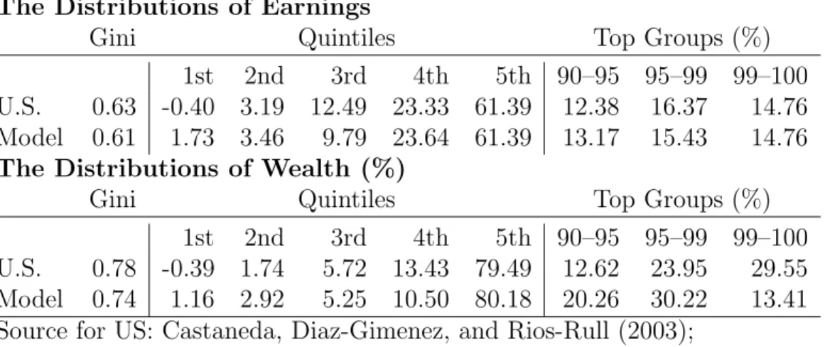
= 31. From an economic point of view, this calibration is interesting because it leads to a rather realistic distribution of income, consumption and wealth (cf. Table 2.5.2).

This calibration matches three targets. The earnings share of the upper quintile of the distribution is 0.6139. The earnings share of the top 1 percent of the distribution is 0.1476.

The conditional annualized variance of persistent income equals 0.15. I assume that from

each grid point ¯ θ

, the household can only switch to neighboring points ¯ θ

,¯ θ

. The

probability with which this happens helps to meet the third target. The probability of

The Distributions of Earnings

Gini Quintiles Top Groups (%)

1st 2nd 3rd 4th 5th 90–95 95–99 99–100 U.S. 0.63 -0.40 3.19 12.49 23.33 61.39 12.38 16.37 14.76 Model 0.61 1.73 3.46 9.79 23.64 61.39 13.17 15.43 14.76

Gini Quintiles Top Groups (%)

1st 2nd 3rd 4th 5th 90–95 95–99 99–100 U.S. 0.78 -0.39 1.74 5.72 13.43 79.49 12.62 23.95 29.55 Model 0.74 1.16 2.92 5.25 10.50 80.18 20.26 30.22 13.41 Source for US: Castaneda, Diaz-Gimenez, and Rios-Rull (2003);

Model calibration of Section 2.5.2.

Table 1: Earnings and wealth distribution in the growth model

reaching the highest state is adjusted so as to meet the second target. To match the first target, the income value of the uppermost 20 percent of grid points is modified upwards from a distribution that is equidistant in logs. To avoid that the distribution drifts too much to the boundaries of the state space, the household faces a constant probability of

“dying”, that means, being reset to the median value of θ. The inverse of this probability is 50 times the model frequency. Transitory productivity ξ

has again two realizations, namely 0.2 and 1.8. This unrealistically high variance of the transitory component helps explaining the lower quintiles of the distribution.

The exact specification of the income process can be seen from the program “caliinc.m”.

2.6 Example 2: An OLG Economy

As a second example, we consider an economy where households have a finite life span, but there is no heterogeneity within cohorts. A household born in period t lives from t to t + T

1. Consumption and labor supply of a household with age i in period t are denoted by c

and l

, respectively. The household supplies one unit of labor in each period before retirement age T

, therefore l

= 1 for i = 0, . . . , T

1 and l

= 0 for i = T

, . . . , T

1.

Labor productivity is normalized to 1/T

, so that total effective labor supply equals 1.

The household born at t maximizes E

T−1

X

i=0

β

u(c

) (25)

Asset holdings follow

k

= R

k

+ W

T

l

c

(26)

The household starts with no assets, and cannot leave debt at the time of dying. The

budget constraint of a household born at t is therefore

k

= 0 (27)

k

0 (28)

Again, there is only one asset (physical capital). The household can save and lend freely in this asset. There is no borrowing or short-sale constraint.

Technological and utility parameters are chosen as in the infinite-life model. To have a model with a similar dimension as before, I choose a monthly frequency and assume 60 years of economic lifetime, so T = 720 and T

= 480. For the OLG model, I only consider technology shocks, specified as in (3). There are no tax shocks (τ

= τ

= 0).

3 Exact and Approximate Aggregation in Linear Mod- els

3.1 Overview of the Solution Method

The method I propose in this paper to compute a numerical solution of heterogeneous agent models (such as the one we have seen in Section 2) involves the following steps:

1. Discretizing the model, as explained in Section 2.4. This usually involves:

•

In a model with a continuum of household, a finite representation of the contin- uous cross-sectional distribution function of the individual state variables such as household assets, cf. Section 2.4.2.

•

A finite parameterization of the continuous decision functions, for example by spline functions of polynomials.

2. Computing the deterministic steady state of the discrete model. This usually involves:

•

In an outer loop, iteration over steady state prices.

•

In an inner loop, computing the optimal decisions of agents conditional on prices, and then finding the ergodic cross-sectional distribution of the individual state variables.

3. Linearizing the model equations around the steady state. This is done by numeric differentiation, either automatic differentiation or some form of finite differences.

4. If the total number of variables in the linearized discrete model is not too big (1000- 2000 on a normal PC), one can compute the solution of the linearized model by any package for linear rational equation systems, for example Sims (2001).

5. If the total number of variables is too big, or if a lower-dimensional approximation

is desired, aggregate the model by state and policy reduction, and solve the reduced

model. We can distinguish two approaches:

(a) Identify the minimal state vector that still allows the model to be solved with very high precision, in the range that the floating-point precision of the computer allows. This will be explained in Section 3.4.

(b) Sacrificing some accuracy, reduce the dimension even further to obtain a small model with reasonable accuracy (in the spirit of Krusell and Smith (1998), Den Haan (2007) and the subsequent literature in macroeconomics). The task then is to find the right set of state variables, in order to obtain (close to) maximal accuracy for a given size of the aggregate model. This will be explained in Section 3.5.

Steps 1–4 have already been described in Reiter (2009b). The topic of the present paper is aggregation (Step 5). As was explained in the introduction, this allows to accurately handle models with a much higher number of variables, and serves as an important input for higher-order solutions.

The linearization in Step 3 gives a solution that is linear in aggregate variables but nonlinear in individual variables. To see what this means, take the growth model as an example. The consumption function, which gives consumption as a nonlinear function of individual assets, is model led as depending linearly on the aggregate state vector, the cross-sectional distribution of capital. If the consumption function is represented by 100 spline coefficients, and the distribution by 1000 histogram values, this linear dependence is described by a 100

1000-matrix.

I would like to stress that in this paper I do not ask whether the discrete model with a high- but finite-dimensional state vector (obtained in Step 1) is a good approximation to the theoretical model with a continuum of agents. This is an important question, which I leave for future work. I rather focus on the question whether the high-dimensional discrete model can be approximated well by a lower-dimensional model. In the following, I will therefore consider the solution to the discrete model as the “exact solution”.

3.2 The Reduced State Space Model

In this section we review some results of the control literature on state aggregation in linear state space models. From Section 3.3 onwards, we will see how to adapt those techniques to the models that are of interest to economists, namely DSGE models.

In the literature on system and control theory, aggregation is called “model reduction”.

We deal with the linear dynamic system

x

= Ax

+ B

(29a)

y

= Cx

(29b)

where A, B and C are given matrices. The vector x contains the state variables, is the

vector of exogenous shocks (“inputs”), which satisfy E

= 0 and E[

] = Σ

. The

vector y is the “output” of the system, the variables that we are ultimately interested in,

and which we observe. The goal then is to approximate (29) by a lower-dimensional model:

ˆ

x

= ˆ Aˆ x

+ ˆ B

(30a)

ˆ

y

= ˆ C x ˆ

(30b)

(29) and (30) are driven by the same shock vector

, and should generate the same output variables. Therefore, y and ˆ y have the same dimension. The idea is to choose the matrices A, ˆ ˆ B and ˆ C so that (30) is a good approximation to (29) in the sense that the response of ˆ y to past in the reduced model is similar to the response of y to past in the original model. State aggregation means that the size of the state vector ˆ x, dim(ˆ x), is considerable smaller than the size of x, dim(x).

A natural way to derive the reduced model (30) is by assuming that the reduced state ˆ

x is linearly related to the original state x by ˆ

x

= Hx

(31)

with appropriately chosen matrix H. We can assume, w.l.o.g., that H is orthogonal:

HH

= I (32)

Notice that H has more columns than rows, so that H

H is not the identity matrix.

Given H, it is natural to choose ˆ A, ˆ B and ˆ C by least squares. OLS estimates of (30) in the model (29) are given by (cf. Appendix B.1)

A ˆ = HAΣ

H

(HΣ

H

)

(33a)

B ˆ = HB (33b)

C ˆ = CΣ

H

(HΣ

H

)

(33c)

where Σ

denotes the unconditional covariance matrix of x. It is given by

(A, B, Σ

), which is defined as the unique symmetric solution to the discrete Lyapunov equation

L

(A, B, Σ

) = AL (A, B, Σ

) A

+ BΣ

B

(34) for any matrices A, B and Σ

of appropriate size such that Σ

is non-negative definite and A is asymptotically stable, which means that all eigenvalues are smaller than unity in absolute value. For the special case of Σ

= I, we will also use the short notation

(A, B).

Appendix B.2 shows that, if A is asymptotically stable, then is ˆ A. The practical compu- tation of Σ

, even in cases where the vector x is very large, is dealt with in Appendix B.3.

When computing the OLS estimates (33), one has to deal with the fact that the matrix HΣ

H

may be ill-conditioned if H has many rows. This can be handled by Tikhonov- regularization,

cf. Appendix B.4

What remains to be done is to find a suitable way of choosing H. The standard approximation method in control theory is called “balanced reduction”. I will explain it as the combination of two ideas: principal component analysis (PCA), and the “conditional expectations approach” (CEA). The latter idea will be of independent interest for us when we consider aggregation in DSGE models.

6I am grateful to Ken Judd for pointing this out to me.

3.2.1 Principal Component Analysis (PCA)

The idea of PCA is to find out in which direction the state vector x varies most strongly.

For that, we consider the eigenvalue decomposition of the unconditional covariance matrix of x, Σ

:

Σ

= USU

(35)

Here, S is a diagonal matrix with the eigenvalues σ

, . . . , σ

, ordered such that σ

σ

. U is the corresponding matrix of eigenvectors of Σ

. (35) decomposes the variance of x into orthogonal components of decreasing importance (principal components). If the sequence σ

σ

decays rapidly enough, one can ignore the components i > k for a suitably chosen k < dim(x). In particular, if σ

is too small compared to σ

, it is numerically indistinguishable from zero. In that case, one can say that the state x lives, up to a very good approximation, in the space spanned by the first k columns of U, which we denote by U

. Then we choose the reduced state ˆ x as the coefficients of x with respect to this basis: x

= U

x ˆ

. Since the columns of U are orthogonal, we can set H = U

and get Hx

= U

U

x ˆ

= ˆ x

, as in (31).

Having chosen H in this way, it can be easily shown that the OLS estimates (33a) reduce to ˆ A = HAH

and ˆ C = CH

.

3.2.2 Conditional Expectations Approach (CEA)

If we are only interested in the variables in y, why is it important to know the full state vector x

? Because x

helps to predict future values y

.We therefore want the reduced model (30) to give us the correct conditional expectations

of future y’s. Then it is natural to include those conditional expectations in the reduced state vector ˆ x. Since

E

[y

] = E

[Cx

], = CA

x

i = 1, 2, . . . (36) this means to set ˆ x

= (CA

)x

for i = 0, . . . , N

1 for some sufficiently large N . Then the reduced model makes the best possible predictions for y

up to N

1 periods ahead.

Moreover ˆ x

predicts not just y

but also ˆ x

for l < i:

ˆ

x

= E

[ˆ x

] = . . . = E

[ˆ x

] = E

[ˆ x

] = E

[Cx

], i < N (37) We might therefore set H equal to

Q(N)













C CA CA

· · ·

CA













(38)

7Notice that in the context of linearized solutions, we do not worry about predictions of higher moments ofyt+i, because the solution is of the certainty-equivalence type in aggregate variables.

But then there is an obvious problem: to have high precision, we need predictions for many periods ahead, and so it seems we need a large vector ˆ x, which contradicts the idea of state aggregation. To get state aggregation, we have to pick k < n

dim(x) rows (or linear combinations of rows) from Q(N ). Mathematical theory suggests

to do this via a singular value decomposition (SVD) of Q(N):

Q(N ) = USV

(40)

where U

U = I, V

V = I, and S is again a diagonal matrix with entries σ

, . . . , σ

, ordered such that σ

σ

. In analogy to the procedure of PCA, we set H equal to the first k rows of V

:

H = V

(41)

We can see a strong formal analogy between CEA and PCA if we consider the limiting case N

Q ≡

∞

X

i=0

∂ E

y

∂x

0

∂ E

y

∂x

=

∞

X

i=0

A

C

CA

= lim

N→∞

Q(N )

Q(N ) =

(A

, C

) (42) The matrix

is called “observability Gramian”, and measures the sum of squares of the contribution of x to the future y’s.

If it is more important to predict the y in the not-too-distant future, then it is better to get H from the SVD of Q(N ) for large N (below I will choose N = 1000, capturing forecasts of the next 250 years) rather then the SVD of

3.2.3 Balanced Reduction

PCA and CEA implement two different ideas on how to reduce the state vector. PCA asks:

“what are the components of x that vary a lot over time”? If a component does not vary, there is no need to include it in the state vector. CEA asks: what are the components of x that help predicting the variables that really matter, namely the future y? If a component of x varies a lot, but this variation is unrelated to changes in y, it is useless to include it in the state vector. The concept of “Balanced Reduction” combines the two approaches.

Define the matrices R, Σ

, Q,

U , S, V , ˜ H as follows:

RR

= Σ

(A, B, Σ

) (43)

QQ

=

(A

, C

) (44)

USV

= R

Q (45)

H ˜ = S

V

Q

(46)

8Given any matrixX with rankn, the rank-kmatrix that is closest to X, both in the L2 and in the Frobenius norm, is given by

X˜ =U S^kV (39)

where U SV is the SVD ofX, andS^k is obtained fromS by zeroing all the singular valuesσⁱ withi > k (Trefethen and Bau III 1997, Theorems 5.8,5.9).

Here, R is the Cholesky factor of the covariance matrix Σ

, and Q is the Cholesky factor of the observability Gramian

U, S and V are the SVD of the matrix R

Q with U

U = I , V

V = I and S diagonal with decreasing entries. We take S as the square matrix containing only the non-zero singular values (and drop the columns of U and rows of V corresponding to the zero singular values), so that S is invertible by construction.

Now consider the variable transformation ˆ x = ˜ Hx, ˆ A = ˜ HA H ˜

, ˆ B = ˜ HB , ˆ C = C H ˜

. Using that ˜ H

= RUS

, straightforward algebra shows that

L

A, ˆ B, ˆ Σ

= ˜ HL (A, B, Σ

) ˜ H

=

A ˆ

, C ˆ

= ( ˜ H

)

(A

, C

) ˜ H

= S. (47) Equ. (47) is a remarkable result. It shows that in the new vector ˆ x the variables are ordered such that ˆ x

has both the i-th highest variance, and makes the i-th highest contribution to future values of y. For the reduced model, we pick the first k components of ˆ x, or the first k rows of ˜ H, such that the diagonal elements S

are negligible for i > k:

H = ˜ H

(48)

3.2.4 Properties of balanced reduction

Is the reduced model (30) an optimal approximation to (29) in any sense? With the choices of H that we have discussed, it is not a strictly optimal. Nevertheless, balanced reduction has a strong performance guarantee (cf. Antoulas (2005, Theorem 7.10), Antoulas (1999, Section 2.6)):

distance(ExactModel, ReducedModel)

2(σ

+ . . . + σ

) (49) Here, the σ’s are the singular values in (45) (called “Hankel singular values”) that were omitted in the construction of H in (48). The distance measure in (49) is the Hankel norm, which is defined as the maximum distance in the future response

v u u t

∞

X

i=0

||yt+i−

y ˆ

(50) to any sequence of past shocks

with unit length:

v u u t

∞

X

i=0

||t−i||²

= 1 (51)

In particular, the difference in the usual impulses responses between exact and the reduced models cannot be bigger than the bound (49). This explains why balanced reduction is the standard aggregation method in the control literature.

There exist even better, but more complicated approximations than balanced reduc-

tion. The theoretical lower bound on the distance between the two models is σ

. This

bound can actually be attained (Antoulas 1999, Sections 2.6.1,3.2). For us, it seems not

worthwhile to investigate more complicated methods, because our main problem is how to

adapt these aggregation techniques to the type of models that we are interested in, namely

linear DSGE models. This is the topic of Sections 3.3 and 3.4.

3.3 The Aggregation Problem in Linear RE Models

The model we want to analyze is given in the form of a linear rational expectations (RE) model, defined through a finite number of equations in a finite number of variables for each model period t. If the original model contains a continuum of state variables, it has first to be discretized. Examples are the discrete models of Section 2.4.3 and A.4. After linearizing this model around the steady state (cf. Section 3.1, Step 3), we assume that the model can be written in the form

x

= T x

+ Dd

+ F

(52a)

d

= E

[E

x

+

x

+

d

] (52b)

y

= Cx

(52c)

with given matrices T , D, F ,

,

,

and C. The vector d contains all the decision variables that are determined by the system of expectational equations (52b). In the stochastic growth models, these are the parameters of the consumption function

, which are pinned down by the household Euler equations. The vector x contains all the other variables. For example, in the growth model, this includes the complete information about the cross-sectional distribution of capital, collected into the vector

, together with Z

and τ

. Again, y

collects the aggregate variables of interest. Notice that it is not restrictive in (52c) to assume that y is a known function of x only, because we can always augment x by elements of y and add corresponding equations to (52a).

The solution to this model is a linear decision function

d

= D

x

+ D

(53) This generates dynamics for the state x of the form (29a), with A and B given by

A = T + DD

(54a)

B = F + DD

(54b)

We assume that (52) has a unique stable solution.

The aggregation techniques of Section 3.2 do not directly apply to models of the type (52), for the following reasons.

1. The dynamics of the model (52) is not known before we solve it, and in general we first have to deal with the aggregation problem before we can solve the model.

In particular, we cannot apply the methods of Section 3.2 that make use of the covariance matrix Σ

.

2. There is a feedback from the aggregation to the solution of the model. If we replace

the state vector x by the reduced vector ˆ x, we assume, explicitly or implicitly, that the

agents in the model base their decision only on ˆ x, not on x. The way we handle the

aggregation problem will therefore have an effect on the solution (53), and therefore

the dynamics of the model.

3. The model may not only have a high-dimensional state x, but also a high-dimensional decision vector d. So we have to think not just of state, but also of policy aggregation.

4. Since economic agents are assumed to base their decisions on ˆ x, we will probably require that ˆ x contains those aggregate variables that are important for the agents’

decision and that we assume are actually observed. So we have to identify those variables and include them into ˆ x.

To handle the last issue, we assume that the vector of aggregate variables y

includes all the aggregate variables that economic agents base their decision on. We therefore require that y

contains at least those variables that enter into equation (52b), and therefore

influence decisions at time t

1 or t. These dependencies are captured in the matrices

and

. While these matrices can be big, it is typically the case that they have very low rank. For example, in the growth model, the state vector x enters the Euler equations (16) only through three variables: the interest rate and the two exogenous states, productivity and capital tax rate. Therefore, the rank of

E_x1 E_x0

equals three. In the SDP model of Section A, this rank is four. That y contains all the decision-relevant variables then means

Ex1 Ex0

∈

span(C) (55)

where span(X) denotes the space spanned by the rows of the matrix X. We further require that complete information about y

is contained in ˆ x

. This means that

C

span(H) (56)

Combining (56) and (55) we get the following requirement on H:

Ex1 Ex0

∈

span(H) (57)

3.4 Exact and Almost-Exact Aggregation in Linear RE Models

3.4.1 Exact State Aggregation

Let us first consider the case that exact aggregation of the linear RE model (52) is possible.

Denote the dimension of x by n. We want to replace x by a state vector ˆ x of dimension k < n. The key condition for exact aggregation is that there exists a k

n-matrix H and a k

k-matrix ˆ T such that

HT = ˆ T H (58)

and H satisfies the spanning requirement (57). We can again normalize H to be orthogonal as in (32). Then we get

T ˆ = HT H

(59)

which is similar to a coordinate transformation. Furthermore, (57) and (32) imply that there exist unique matrices

and

such that

Ex0

=

H (60a)

E_x1

=

H (60b)