DISCUSSION PAPER SERIES
Forschungsinstitut zur Zukunft der Arbeit Institute for the Study of Labor
Human Capital Investments in Children:
A Comparative Analysis of the Role of
Parent-Child Shared Time in Selected Countries
IZA DP No. 5084
July 2010 Eva Österbacka Joachim Merz Cathleen D. Zick
Human Capital Investments in Children:
A Comparative Analysis of the Role of Parent-Child Shared Time in
Selected Countries
Eva Österbacka
Åbo Akademi University and Kela
Joachim Merz
Leuphana University Lüneburg, FFB and IZA
Cathleen D. Zick
University of Utah
Discussion Paper No. 5084 July 2010
IZA P.O. Box 7240
53072 Bonn Germany
Phone: +49-228-3894-0 Fax: +49-228-3894-180
E-mail: iza@iza.org
Any opinions expressed here are those of the author(s) and not those of IZA. Research published in this series may include views on policy, but the institute itself takes no institutional policy positions.
The Institute for the Study of Labor (IZA) in Bonn is a local and virtual international research center and a place of communication between science, politics and business. IZA is an independent nonprofit organization supported by Deutsche Post Foundation. The center is associated with the University of Bonn and offers a stimulating research environment through its international network, workshops and conferences, data service, project support, research visits and doctoral program. IZA engages in (i) original and internationally competitive research in all fields of labor economics, (ii) development of policy concepts, and (iii) dissemination of research results and concepts to the interested public.
IZA Discussion Papers often represent preliminary work and are circulated to encourage discussion.
Citation of such a paper should account for its provisional character. A revised version may be available directly from the author.
IZA Discussion Paper No. 5084 July 2010
ABSTRACT
Human Capital Investments in Children:
A Comparative Analysis of the Role of Parent-Child Shared Time in Selected Countries
Parents invest in their children’s human capital in several ways. We investigate the extent to which the levels and composition of parent-child time varies across countries with different welfare regimes: Finland, Germany and the United States. We test the hypothesis of parent- child time as a form of human capital investment in children using a propensity score treatment effects approach that accounts for the possible endogenous nature of time use and human capital investment. Result: There is considerable evidence of welfare regime effects on parent-child shared time. Our results provide mixed support for the hypothesis that non- care related parent-child time is human capital enriching. The strongest support is found in the case of leisure time and eating time.
JEL Classification: D1, J24, J22, H43
Keywords: parent-child time, comparative research, welfare regimes, Finland, Germany, USA, treatment effects, propensity score matching
Corresponding author:
Joachim Merz
Leuphana University Lüneburg Department of Economics
Research Institute on Professions (FFB) 21332 Lüneburg
Germany
E-mail: merz@leuphana.de
2
1. Introduction
How is it that parents invest in their children’s human capital and are their investment choices linked to the investment choices that the larger society makes in children? While an
extensive literature documents the out-of-pocket investments that parents make, much less is known about their time-related investments. The few studies that link parental time to children’s human capital development focus on parent-child time spent in specific activities such as shared leisure (e.g., cultural events, sporting activities), educational activities (e.g., helping with homework), and/or eating time. These studies document the positive relationship between the time parents share with children in non-care activities and developmental benefits within a single country (Buchel &
Duncan 1998, Zick et al. 2001, Dubas & Gerris 2002, Crosnoe & Trinitapoli 2008).
Other scholars have undertaken comparative time use studies with the goal of assessing how different social welfare regimes affect parents’ time use, particularly child care time (Sayer et al.
2004, Craig 2005). Sayer and her colleagues find support for the hypothesis that welfare regimes influence both the level and relative contributions of mothers and fathers to child care time. Craig also finds that being a parent affects the workload differently across different welfare regimes. To date, no one has examined how government supports might affect parental time spent in non-care related activities such as shared leisure, shared meals, and shared housework. Yet, the literature suggests that when parents engage children in such activities they may be undertaking important human capital investment.
The current research builds on the existing literature in three important ways. First, we describe parental time spent with children in potentially human capital enriching activities with the goal of presenting a more complete portrait of shared time – both in terms of the total amount and its composition. Second, we investigate the extent to which the levels and composition of parent-
3 child time (excluding child care time which as been studied by Sayer et al, 2004 and Craig, 2005) varies across countries with different welfare regimes. Specifically, we compare parental time use in countries that represent the three welfare regimes laid out by Esping-Andersen (1999). Finally, we test the hypothesis of parent-child time as a form of human capital investment in children using a propensity score treatment effects approach that accounts for the possible endogenous nature of time use and human capital investment.
2. Human Capital Investment – Shared Time with Children
Each child inherits an initial human capital endowment from her/his parents. However, of crucial importance to a child's development are the subsequent investments that are made in her/his human capital. Both parents and the public sector act as investors during the crucial period of early childhood. Becker and Tomes (1986) argue that if parental and public investments are perfect substitutes, parental investments will be crowded out as public investments expand. If parental and public investments are not perfect substitutes, public investments might still affect parental
behaviors. Regardless, the idea that parental and state investments are important inputs in their children’s human capital is beyond dispute. Parents invest time, money, and emotional energy in their children.1 The most directly observable form of public investment in children is education.
However, the public sector also invest considerable resources in children through the choices that the politicians make about subsidies for financial support for health care, work-related child care, and other forms of family policies.
We assume that all parents want to insure that their children acquire some optimal level of human capital. Yet, countries with different welfare regimes are different in the way family life, the labor market and the public sector are organized. These differences may alter the decisions that parents make about the time they spend with their children in potentially human capital enhancing
4 activities. Social democratic governments generally provide the greatest resource supports to families and children, followed by conservative governments, and lastly by liberal governments (Esping-Andersen, 1999). If welfare states are viewed as a predetermined characteristic of the family environment that potentially substitutes for parental human capital investments, then we would expect that parents in social democratic countries would spend the least time investing in their children, followed by parents in conservative countries, with parents in liberal countries spending the most time investing in their children. To test the proposition that welfare regimes impact parent-child time, we examine potentially human capital enriching parent-child time in Finland, Germany, and the United States as prominent welfare regime countries.
Ideally, our analyses would make use of longitudinal data where time spent with parents in a child’s early years is linked to human capital-related child outcomes at a later point in time (e.g.
linking parental time spent with a child during the early years to a child’s ultimate educational attainment using a panel econometric approach). Unfortunately, there are not any panel study time diary data sets currently available. Thus, we must fall back on the use of cross-sectional time diary data. The use of cross-sectional data to investigate questions of time use and human capital investment raises issues about the possibility of endogenity of parental choices about how they spend their time and whether or not their time should be shared with a child.2
Concern about the potential dependence between time allocation and the decision to share certain types of time with children would disappear if eligible respondents were randomly assigned to have a child present during specific activities. But, they are not. Rather, respondents self-select as to how much time they spend in certain activities and that self-selection may be related to whether or not a child is present. One approach to this self-selection issue would be to estimate a simultaneous system. This strategy is limited by the functional form that is chosen and by the reality that such methods may hide the fact that many in the “treated” sample have no
counterfactual in the non-treated sample (i.e., there is a lack of common support) (Black & Smith, 2004; Gibson-Davis & Foster, 2006).
5 Rosenbaum and Rubin (1983, 1984) propose the use of the propensity score method which approaches the simultaneity problem by balancing a treatment group (i.e., parents participating in an activity with one or more children under age 10 present during the activity; the treatment thus is the presence of those children) with a control group (i.e., parents participating in the same activity with no children under age 10 present) with regard to their covariates. Essentially, the propensity score adjusts for the bias that may be caused by certain types of parents self-selecting into doing certain activities when children are present by creating matches between members of the treatment and control groups rather than through the random assignment that is used in true experiments (Angrist
& Pischke, 2009).
The propensity score approach relies on first estimating a logit type equation where the dependent variable is the presence or absence of a child under age 10 during an activity spell
{ }
(
D= 1,0)
. The independent variables in the logit model, X , include factors that might affect whether or not the child is present as well as factors that might affect how much time is spent in the activity. The specification of the functional form and the independent variables can vary as the goal is simply to maximize the predictive capabilities of the model. However, we include content driven explanatory variables which in addition should minimize possible unobserved heterogeneity. From the logit estimates, the predicted probabilities of having a child present while participating in an activity are generated for all respondents. These predicted probabilities become the features on which treated parent-child spells are matched to control spells of parental time.Next, a common support region is defined and only those observations that fall within this region are further analyzed. The common support region is defined by the area of overlap in propensity scores for the treated and untreated groups. Within the common support area, members of the treatment group are matched to members of the control group. A number of matching methods are used in the literature and these methods reflect the tradeoffs one must make between bias and variance when matching with small sample sizes (Gibson-Davis & Foster, 2006; Caliendo and Kopeinig, 2008). However, when sample sizes are large, the various matching approaches
6 should produce similar results. Once the matching is complete, t-tests are conducted to ascertain if statistically significant differences exist between the treatment and the control groups with respect to spell length.3
In our application, if the length of the spell of each activity is dependent on the presence (absence) of a child after adjusting for the propensity score, this becomes a weak test of human capital investment. That is, such a result would be consistent with the hypothesis that parents will spend more time in an activity when a child is present because they are using some of that time to invest in the child’s human capital (e.g., talking with the child while eating dinner, teaching a child how to cook while making dinner). It is a weak test because differences in spell length could also reflect differences in the current consumption value of engaging in an activity with or without a child. For example, meals may simply be more (or less) enjoyable for a parent when they are eaten with a child present and this leads the parent to devote more time to eating.
In using the propensity score approach, we are estimating the population average treatment effect on the treated (ATT). This is the causal effect of treatment only on that group and not the overall treatment effect. Treatment (control) in this case is the presence (absence) of a child under age 10 during an activity spell, (D=
{ }
1,0 , where 1=child present and 0=child not present). The outcome is the length of the spell in minutes(
Y ={
Y1,Y0} )
. The causal effect of treatment is defined as ∆ATT =Y1 −Y0. The mean of ∆ATT is defined according to:(
∆ | =1)
=(
1− 0| =1) (
= 1| =1) (
− 0 | =1)
=
∆ATT E ATT D EY Y D EY D EY D (1)
However, as equation (1) is formulated, it cannot be estimated because we do not have both the treated and non-treated spell length for one person at the same time. Hence the last term is not determinable.
To make the estimation tractable, three conditions must hold. First, once we control for
7 observable covariates, X, so that the potential outcome is independent of the treatment selection.
This is known as the conditional independence assumption (CIA). This assumption allows the means of ∆ATT to be estimated by using E
(
Y0 |D=0,X = x)
instead of E(
Y0|D=1,X =x)
inequation (1). The conditional independence assumption (CIA) can be formalized according to:
X D
Y0 ⊥ | (2)
In our case, this means that the presence of a child should random after we control forX. We meet the CIA assumption by doing two things. First, we include inX , both parental and child
characteristics that have been found to be associated with time spent with children (Buchel &
Duncan 1998, Zick et al. 2001, Dubas & Gerris 2002, Sayer et al. 2004, Craig 2005, Crosnoe &
Trinitapoli 2008). We follow the specification of past research as closely as possible across all three analyses given the limits on the information available in each of the three time diary data sets we utilize. Second, we focus on parental time-use activities that are done whether or not a child is present (i.e., eating, housework, watching television, leisure, transportation). It is arguable that often a child may be off playing with friends, at school or engaged in other leisure activities away from the parent. This allows for the possibility that the child’s presence during a specific activity may be somewhat random. To the extent that spells with children may be a function of structural factors, we include among our covariates measures of structural aspects of the spell characteristics including time of day, day of week, and season of the year. We assess whether or not these actions help us meet the CIA requirement by conducting t-tests to assess if the distribution of theX is the same between the treated and untreated groups (Caliendo and Kopeinig, 2008).
The second condition that must be met is the common support assumption. That is, the estimated probabilities of participation for the treatment group must overlap with the estimated probabilities of participation for the control group and the probabilities have to be positive, irrespective of the value of X (Imbens, 2004, Smith & Todd, 2005, Caliendo & Kopeinig, 2008).
8 To meet this condition, we drop treatment observations whose pscore is higher than the maximum or less than the minimum of the controls. Once the common support region criterion has been satisfied, we use nearest neighbor matching with replacement to pair spells in the treated group (i.e., child present for the specified activity) with spells in the non-treated group (i.e., child not present for the specified activity). Our sample sizes are relatively large and thus nearest neighbor matching with replacement should produce unbiased results that are quite similar to other matching methods although the variance may be increased (Caliendo and Kopeinig, 2008).4 As such, this matching technique provides a conservative test.
The final condition that must be met in order to estimate the ATT is the stable unit treatment value assumption (SUTVA). SUTVA requires that the outcome of a unit depends on the own participation only and not on the treatment of the other units. Satisfying SUTVA would be a
problem if we pooled mothers and fathers from the same family in our analyses. To avoid violating this assumption, we estimate propensity scores separately for mothers and fathers. This approach also insures perfect matching on gender (Heckman, Ichimura, Smith, and Todd, 1998).
3. Data Sets
We construct compatible time diary data sets for Finland, Germany, and the United States given the limitations that are inherent in each data set’s design. Specifically, we restrict our samples to respondents with complete time diaries, who are between the ages of 20 to 60, who are married or cohabiting, and who have one or more minor children under the age 10 present in the home.
The Finnish Time Use Survey (FTUS) was conducted in 1999-2000 by Statistics Finland.
The FTUS design follows EUROSTAT’s Guidelines on Harmonised European Time Use Surveys (HETUS). The survey is a representative sample covering persons aged 10 and above. The data included 5,300 individuals from 2,600 households. Participants were asked a series of questions
9 regarding their personal characteristics and one household member was asked about the household characteristics. Some register information regarding their income was added to the survey. All respondents were asked to fill in a time use diary based on 10-minute intervals for two days, one weekday and one weekend. For each 10-minute spell, respondents filled in their primary activity and what else they were doing at the same time. They were also asked to fill in with whom they spent their time, the location and mode of transportation. For this data set, the information on with whom respondents spent their time was not available for those respondents interviewed in January and February. Hence, observations from those two months are missing (Niemi and Pääkkönen, 2001). Our present sample consists of 329 fathers and 363 mothers.
The German Time Use Survey (GTUS) of 2001/02 provided by the German Federal Statistical Office consists of about 5,400 households and approximately 37,700 diary days. The GTUS design also follows EUROSTAT’s Guidelines on Harmonised European Time Use Surveys (HETUS). All household members aged 10 years and older were asked to fill out diaries based on 10-minute intervals on three days – two days during the week from Monday to Friday, one day on the weekend. Data were collected on primary and secondary activities, persons involved or present, the location and mode of transport. Household and individual data (i.e., socio-demographic/econo- mic variables and other background variables) were collected in additional questionnaires. A comprehensive GTUS-Compass about the broad range of GTUS 2001/02 information and its usage is provided by the German Federal Statistical Office (Statistisches Bundesamt, 2006). There are 890 fathers and 890 mothers in the sample used for the current analysis.
The third time diary data set is the 2003 American Time Use Survey (ATUS). The 2003 ATUS is the first annual American time-diary survey conducted by the U.S. Bureau of Labor Statistics and thus the closest ATUS survey to the Finnish and German data. Each year a sample is drawn from those households that have completed the final interview for the Current Population Survey. The ATUS respondent is randomly selected from among each household’s members who are age 15 or older. Respondents are asked a series of questions that focus on household
10 composition, employment status, etc. They are also asked to complete one 24-hour time diary using retrospective recording methods. Half of the respondents complete a diary for a weekday and half of the respondents complete a diary for a weekend day. For each activity the respondent reports doing over the 24 hours, s/he is also asked who else was present when doing the activity. For the current analyses our sample consists of 2,416 mothers and 2,136 fathers, who had no missing data on the
“who with” question.
Both the FTUS and GTUS are part of the Harmonized European Time Use Survey, where activities are comparable by design. We use the ATUS survey coding lexicons to create comparable activity categories with the FTUS and GTUS.
In all the time use surveys, one diary day consists of information on activities during a 24 hour period. We do not use all information on the performed activities; the activities of interest in our analyses are spells of eating, housework (where child care is not included), leisure (where television and video viewing is not included), and television and video viewing. These activities may be considered child care in the broadest sense (Klevmarken, 1999) but they are not seen as traditional child care when coding the parent’s time. Thus, for each type of activity we examine whether or not a child was present during a spell and how long the spell lasted.
Individuals in the surveys can have multiple spells of each activity during the 24-hour diary period and in two of the three surveys, each individual has more than one 24-hour diary. Thus, all analyses correct for the correlation of error terms caused by having multiple spells from the same individual included in the analyses. In addition, all descriptive information is weighted using the weights provided in each data set. The multivariate analyses are not weighted as these analyses control for those factors used to construct the sampling weights (DuMouchel and Duncan, 1983).
11
4. Results – Human Capital Investments in Children
We focus on primary time in eating, housework leisure, and TV/video time because we believe they are the most common non-care related activities that offer the potential for parents to engage in child-related human capital investment. Parents may talk to a child about his/her day or about current events, etc. over a meal, or even while engaging in leisure activities. Likewise, life skills may be taught by a parent while doing housework with a child or engaging in active leisure (e.g., playing a sport) with a child. Admittedly, it is less likely that human capital investment occurs when a parent watches television or a video with a child. But, even television/video viewing may provide a parent with some “teachable moments”.
In Table 1, mean daily times spent in the selected activities are presented for the samples in order to give some background to our analyses. On average, German parents spend the most time in eating while the parents in the United States spend the least time in eating. Mothers clearly spend more time in housework than fathers in all three countries, and German parents are the most diligent in devoting time to housework. Parents in the United States spend the least time in housework, and Finnish parents are in between. Parents in the United States spend less than two hours per day on average in leisure activities, while parents in Finland and Germany spend around two and a half hours per day. At the same time, parents in the United States generally spend somewhat more time watching TV than their counterparts in Finland and Germany. Though the overall picture across the three countries is heterogeneous, differences with regard to the amount of activity time can be recorded.5
When it comes to shared time, German parents also spend the most time eating with children under 10 years old on average, while they share relatively smaller amounts TV viewing time.
Parents in the United States, share more TV watching and generally share less eating and less housework time than their counterparts in Finland and German. Finnish parents on the other hand, share housework for longer periods with children under 10 years old on average than other parents but their shared time spent eating with children is shorter.6
12 Times spent in the four selected activities are not spent consecutively; rather they are spent in several spells over the course of the day. Table 2 shows the mean times for spells in the four different activities by whether or not a child less than age 10 was present.
Table 2 also provides preliminary evidence regarding the effect of welfare regimes on parent-child shared time. Focus on the rows that report spells spent with one or more children under age 10. These rows reveal that shared parent-child spells for eating, housework, leisure, and TV viewing are all longest for mothers and fathers in the United States, and the differences are statistically significant. German parents’ average spell length for eating and leisure time is in the middle and Finnish parents’ average spell lengths are the shortest. Spell length for housework and TV watching are not statistically different between Finnish and German parents.7 However, if parental time spent in these four activities involves some human capital investment on the part of their children, then these differences are consistent with what is predicted by Esping-Andersen’s (1999) welfare regime typology.
Comparing the spells with children present to the spells without children present reported in Table 2, we observe that spell length for the four activities in question is generally shorter for Finnish mothers and fathers when one or more children under age 10 is present compared to when no children are present, the only non significant difference is eating time. In contrast, in Germany, the eating and leisure spells for mothers and fathers are longer when children are present relative to when they are not present, and the opposite holds for housework and TV watching. Finally, in the United States, the spells are relatively longer when one or more children under age 10 are present, with the exception of housework for fathers where the difference is not significantly different.8 This pattern across countries is again consistent with the prediction that government supports may substitute for some parental human capital investments in social democrat countries like Finland.
To more confidently assess whether or not shared parent-child time in non-care activities involves human capital investment, we must move beyond the bivariate comparisons in Table 2 for two reasons. First, the observed bivariate relationships could be spurious if family socio-
13 demographic characteristics also vary across these three countries. Second, parents may self-select into shared versus non-shared time use spells. To address these two potential shortcomings, we contrast the above findings with the results obtained using a treatment effects approach by propensity score methods where similar parents are matched and their time use is compared.
In Table 3, the results for a nearest neighbor matching propensity scores are presented.9 With regard to the matching quality, the common support assumption is met as there is a broad overlapping score region for all activities in each country.10 There are generally more treated relative to the untreated respondents when the probability of time shared with a child is higher which is in some favor of our maintained hypothesis. We also test the resemblance of the covariates in the treated and control groups in all activities. After matching, the respective means of the covariates for each country are very close which empirically supports the CIA. The significant bias reduction of the matched covariates and the valid null hypotheses of no differences of the matched covariate means of the treated and the control group supports the argument of a successful matching procedure with important and central explanatory variables by the selection on observables in the logit estimates behind.11
Turning to the propensity score results presented in Table 3, focus first on eating time. Time spent eating is thought to be enriching if it is done with family members in part because of the nutritional and eating habits it can convey and because it provides parents with an opportunity to engage their child(ren) in conversation. Family members relate events of the day, plan and coordinate future activities, discuss their accomplishments and frustrations, etc. When family members eat together, they typically also eat a more balanced and nutritious meal (Neumark- Sztainer, et al., 2003; Eizenberg, et al., 2004; Traveras, et al., 2005; Spear, 2006). As our results in Table 3 suggest, fathers in all three countries spend significantly more time in eating spells if a child less than 10 years old is present. The largest increases in shared eating time are for fathers in the U.S. followed by German fathers and then by fathers in Finland. The results for mothers are
14 more mixed with only German mothers spending significantly more time. The rank ordering for the fathers is in keeping with the hypothesized impact of the different welfare regimes.
Housework may be a form of human capital investment if the child is well supervised. The
parent can teach the child specific tasks, the child learns cooperative behavior, and it fosters responsibility. At the same time, the child also learns gender-specific behaviors and gains an awareness of the family's socioeconomic status (see Goodnow, 1988 for an overview). Yet, Table 3 reveals that Finnish and German mothers and fathers, along with American fathers, all spend less time in housework if one or more children under age 10 are present (although the estimates for Finnish mothers, German fathers, and American fathers do not reach conventional levels of statistical significance). Only American mothers spend more time in housework spells when a young child is present, suggesting that they may be the only parents who view such time to be human capital enriching.
It is important to note that we cannot tell from these data whether or not the children are helping with the chores. We only know that they are present. Thus, a number of stories are consistent with our findings. It may be that children in Finland and Germany are more helpful in doing the chores (allowing their parents to finish more quickly), while the presence of children in the United States, dampen their mothers’ housework productivity. Alternatively, it may be that mothers in the United States are simultaneously teaching their children how to do the tasks which may decrease their productivity in the short run but enhance their children’s human capital in the long run. In any case, the marginal differences in spell length are small. More confident
conclusions regarding these cross-country differences can only be ascertained with data (either qualitative or quantitative) that examines not only the time inputs but also the household production outputs.
Leisure activities can also be a form of human capital investment. Play can promote positive development, including cognitive, linguistic, social and emotional development. Structured
activities like sports, arts, music, hobbies, and organizations offer high challenge, concentration,
15 and motivation (Larson, 2001). The coefficients for Finnish parents are negative, however only statistically significant for mothers (-7 minutes). On the other hand, both German and American mothers and fathers spend significantly more time in leisure activities if one or more children under age 10 are present. The sizes of the estimated time differences are larger for the American parents.
The differences we observe across the three countries are consistent with the differences we would expect across the welfare regimes if leisure time includes an element of human capital investment.
TV/video watching is not typically associated with positive developmental experiences for
children. Unsupervised and for long hours, it is associated with among other things obesity, lower school grades and aggressive behavior (Larson, 2001). But, if a parent watches TV/video together with a young child it may be a more positive activity. Both Finnish and German parents spend significantly less time watching TV/videos if a child less than 10 years old is present, and the magnitude of these differences is fairly large (Finns 7-12 minutes and Germans 25-39 minutes less time). In contrast, parents in the United States watch 5-11 minutes more TV if a child is present (although the estimate for mothers not significant). The negative estimates associated with shared television viewing time in Finland and Germany are consistent with the general view that
television/video viewing does not promote positive developmental outcomes. In the case of the American parents, the positive difference might be interpreted as a human capital investment if the program they watch with their children is educational or generates parent-child discussion. But, more likely, the change in signs simply reflects American adults’ greater relative preference for television viewing over other leisure activities.
5. Summary and Conclusions
The aim of our study is to analyze the impact of government welfare regimes on parental human capital investments in children. We use time diary data from Finland to represent a social
16 democratic welfare regime, Germany to represent a conservative welfare regime, and the United States to represent a liberal welfare regime. We assess non-care related human capital investment time by focusing on the time parents share with their children in four potentially enriching time use categories: eating, housework, leisure (excluding TV), and television/video viewing. In the
multivariate analyses we control for other possible confounding socio-demographic factors and we adjust for possible endogeneity using propensity score techniques. We compare the impacts on time spent in selected activities for treatment (child present) and non-treatment groups (child not present) by nearest neighbor matching. In both the bivariate and the multivariate analyses, we find considerable evidence of welfare regime effects on parent-child shared time.
Our results provide mixed support for the hypothesis that non-care related parent-child time is human capital enriching. The strongest support is found in the case of leisure time (both parents in Germany and the U.S.) and eating time (fathers only in all three countries). For these two categories we see that the presence of children is typically associated with longer spells and this result is consistent with the human capital investment hypothesis. Our results for housework and television/video viewing time provide no support for the human capital enrichment argument. In the case of television/video viewing time, the result is not surprising. The absence of support for shared housework as human capital enriching may reflect the more general trend away from investing in domestic skills. In recent years, advances in household technology and the growing availability of paid housekeepers have increasingly substituted for family members’ housework time in many countries thus reducing the need for individual family members to possess high levels of household production related human capital.
Our hypothesis that parents and government may serve as substitutes with respect to
children’s human capital investment also finds mixed support in our analyses. Focus only on eating and leisure time where we have support for the human capital investment hypothesis. If government programs substitute for parental investments, then we would expect to see Finnish parents spending the least amount of time investing in their children’s human capital, followed by German parents,
17 and finally by U.S. parents. Yet, the descriptive results suggest that, on average, German parents spend the most time eating with their children with the Finns and Americans spending similar amounts of time in this activity. In the case of leisure time, the Americans do average more shared leisure than the Germans and Finns which is consistent with our hypothesis. But, there is little difference between German and Finnish parents. The propensity score analyses show that in the case of fathers’ eating time, the relative magnitude of the shared time effects across the three countries are as we predicted although the absolute effect sizes are small. The strongest support for the regime effect hypotheses can be seen in the shared leisure time propensity score analyses where the incremental amount spent in shared leisure is largest for mothers and fathers in the U.S.,
followed by the German parents, and then the Finnish parents. Thus, if welfare regimes influence parents’ choices about time spent investing in their children’s human capital, they appear to do so only through parental choices about shared leisure activities.
Our findings and interpretations must be circumscribed by several considerations. First, while our analyses control for a number of individual and household factors, we are unable to control for all socio-cultural and political differences that might influence parental time use in Finland, Germany, and the United States. We are also unable to control for more localized welfare regime effects (i.e., state or local differences in government sponsored social support programs).
Thus, differences in the welfare regimes across these three countries are only one possible interpretation of our findings.
Second, data constraints also limit our analyses. Specifically, the relatively small Finnish sample may contribute to the lack of statistical significance in some analyses. In addition, we restrict shared parent-child time to those spells where one or more children under age 10 are present because the Finnish data set did not include information on shared time with older children.
Consequently, we do not know if our results generalize to situations where older children are present.
18 Finally, we interpret the positive differences in shared eating and leisure activities to be an indication of parental investment in children’s human capital. Another interpretation of these findings would be that parents simply place a higher value on the consumption aspects of shared time spent eating and engaging in leisure. Clearly, a more definitive test of parental investment in children’s human capital would involve linking such time to specific child outcome measures.
Future research should address these shortcomings as new comparative data from countries operating with different social welfare regimes becomes available.
19
References
Angrist, Joshua D. and Jörn-Steffen Pischke. 2009. Mostly Harmless Econometrics – An Empiricist’s Companion. Princeton University Press. Princeton and Oxford.
Becker, S. Gary and Nigel Tomes. 1986. Human Capital and the Rise and Fall of Families. Journal of Labor Economics 4(3):S1-S39.
Bianchi, Suzanne M. 2000. Maternal Employment and Time with Children: Dramatic Change or Surprising Continuity? Demography 37(4):401-414.
Black, Dan A. and J.A. Jeffery Smith. 2004. How Robust is the Evidence on the Effects of College Quality? Evidence from Matching. Journal of Econometrics, 121(1-2): 99-124.
Bryant, W. Keith, and Cathleen D. Zick. 1996. Are We Investing Less in the Next Generation?
Historical Trends in Time Spent Caring for Children. Journal of Family and Economic Issues 17(3/4):365-392.
Buchel, Felix, and Greg J. Duncan. 1998. Do Parents' Social Activities Promote Children's School Attainments? Evidence from the German Socioeconomic Panel. Journal of Marriage &
Family 60(1):95-108.
Caliendo, Marco, and Sabine Kopeinig. 2008. Some Practical Guidance for the Implementation of Porpensity Score Matching. Journal of Economic Surveys, 22(1): 31-72.
Chalasani, Satvika 2007. The Changing Relationship between Parents’ Education and their Time with Children. electronic International Journal of Time Use Research, Vol. 4, No. 1, 93- 117.
Craig, Lyn. 2005. Cross-national comparison of the impact of children on adult time. SPRC Discussion Paper No. 137. Social Policy Research Centre.
Crosnoe, Robert, and Jenny Trinitapoli. 2008. Shared Family Activities and the Transition From Childhood Into Adolescence. Journal of Research on Adolescence (Blackwell Publishing Limited) 18(1):23-48.
Dubas, Judith Semon, and Jan R. M. Gerris. 2002. Longitudinal Changes in the Time Parents Spend in Activities With Their Adolescent Children as a Function of Child Age, Pubertal Status and Gender. Journal of Family Psychology 16(4):415-427.
DuMouchel William, H, and Duncan Greg J. 1983. Using Sample Survey Weights in Multiple Regression Analyses of Stratified Samples. Journal of the American Statistical Association.
78(383):535-43.
Eizenberg Marla E., Rachel E. Olson, Dianne Neumark-Sztainer, Mary Story, and Linda H.
Bearinger. 2004. Correlations between Family Meals and Psychosocial Well-being among Adolescents. Archives of Pediatrics and Adolescent Medicine. 158: 792-796.
Esping-Andersen, Gøsta. 1999. Social Foundations of Postindustrial Economies. Oxford University Press. Oxford.
Gauthier, Anne H., Timothy M. Smeeding, and Frank F. Furstenberg Jr. 2004. Are Parents
Investing Less Time in Children? Trends in Selected Industrialized Countries. Population &
Development Review 30(4):647-671.
Gibson-Davis, Christina M. and E. Michael Foster. 2006. A Cautionary Tale: Using Propensity Scores to Estimate the Effect of Food Stamps on Food Insecurity. Social Science Review, 93-126.
Goodnow, J. Jacqueline, 1988, “Children's Household Work: Its Nature and Functions”
Psychological Bulletin. 103(1):5-26.
Heckman, James, Hidehiko Ichimura, Jeffery Smith, and Petra Todd. 1998. Characterizing Selection Bias Using Experimental Data. Econometrica. 66:1017-1098.
Imbens, Guido W. 2004. Nonparametric Estimation of Average Treatment Effects under Exogeneity: A Review. Review of Economics and Statistics, 86(1): 4-29.
20 Klevmarken, Anders. 1999. Microeconomic Analysis of Time Use Data: Did We Reach the
Promised Land? in Merz, J. and M. Ehling (Eds.). Time Use – Research, Data and Policy.
Publications of the Research Institute on Professions (Forschuingsinstitut Freie Berufe, FFB) Vol. 10, NOMOS Publisher: 423-456
Larson W. Reed, 2001. How U.S. Children and Adolescents Spend Time: What It Does (and Doesn't) Tell Us About Their Development. Current Directions in Psychological Science 10(5):160-164.
Leuven, Edwin and Barbara Sianesi. 2003. PSMATCH2: Stata Module to Perform Full
Mahalanobis and Propensity Score Matching, Common Support Graphing, and Covariate Imbalance Testing.
Niemi, Iiris and Pääkkonen, Hannu. 2001. Ajankäytön muutokset 1990-luvulla. Helsinki:
Tilastokeskus.
Neumark-Sztainer, Diane, Peter J. Hannan, Mary Story, Jillian Croll, and Cheryl Perry. 2003.
Family Meal Patterns: Associations with Sociodemographic Characteristics and Improved Dietary Intake among Adolescents. Journal of the American Dietetic Association. 103:317- 322.
Rosenbaum, Paul R. and Donald B. Rubin. 1983. The Central Role of the Propensity Score in Observational Studies for Causal Effects. Biometrika, 70(1): 41-55.
Rosenbaum, Paul R. and Donald B. Rubin. 1984. Reducing Bias in Observational Studies Using Subclassification on the Propensity Score. Journal of the American Statistical Association, 79(387): 516.
Sandberg, John F., and Sandra L. Hofferth. 2001. Changes in Children's Time with Parents: United States, 1981-1997. Demography 38(3):423-436.
Sayer, Liana C., Anne H. Gauthier, and Frank F. Furstenberg. 2004. Educational Differences in Parents' Time with Children: Cross-national Variations. Journal of Marriage & Family 66(5):1152-1169.
Smith, Jeffery A., & Todd, Petra E. 2005. Does Matching Overcome LaLonde’s Critique of Nonexperimental Estimators? Journal of Econometrics, 125(1-2): 305-353.
Spear, Bonnie A. 2006. The Need for Family Meals. Journal of the American Dietetic Association.
106(2): 218-219.
Statistisches Bundesamt (Ed.) 2006, Compass 2001/02 Time Use Survey: Publications, Links and Prints incl. Data Files and Research Facilities, Federal Statistical Office Germany,
Wiesbaden.
Traveras Elise M., Sheryl L. Rifas-Shmin, Catherine S. Berkey, Helaine R.H. Rocket, Alison E.
Field, A. Lindsay Frazier, Graham A. Colditz, and Matthew W. Gillman. 2005. Family Dinner and Adolescent Overweight. Obesity Research. 13:900-906.
Zick, Cathleen D., W. Keith Bryant, and Eva Österbacka. 2001. Mother's Employment, Parental Involvement, and the Implications for Intermediate Child Outcomes. Social Science Research 30(1):25-49.
21 Table 1. Weighted Mean daily duration (in minutes) in selected activities in Finland, Germany and the United States.
Finland Germany United States Activity Fathers Mothers Fathers Mothers Fathers Mothers
Eating 78 78 96 106 58 59
Eating with children < 10 36 50 61 78 39 46
Housework 114 218 161 283 93 179
Housework with children < 10 40 112 36 96 28 76
Leisure 152 145 165 166 99 95
Leisure with children < 10 55 71 54 68 48 54
TV 110 92 104 82 123 104
TV with children < 10 38 45 15 15 54 55
N diary days 623 695 2666 2668 2256 2583
N observations 329 363 890 890 2256 2583
Sources: FTUS 1999-2000. GTUS 2001/02, ATUS 2003
22 Table 2. Weighted Mean Times for Spells Spent in Various Activities by Presence/Absence of One or More Children under Age 10.
Finland Germany United States
Fathers Mothers Fathers Mothers Fathers Mothers
Mean N
Spells N Respon- dents
Mean N Spells
N Respon -dents
Mean N Spells
N Respon -dents
Mean N Spells
N Respon -dents
Mean N Spell s
N Respon -dents
Mean N Spells
N Respon -dents All Spells
Eating 22.85 2173 326 21.13 2574 363 31.32 8203 890 30.53 9333 890 32.98 3787 2000 33.41 4557 2355 Housework 31.63 2364 310 29.58 5105 363 31.15 13721 888 31.94 23791 890 49.50 3898 1521 38.00 10950 2374 Leisure 45.26 2200 320 37.00 2819 361 50.95 8665 887 44.81 10010 888 69.11 3071 1519 61.65 4010 1833 TV 53.32 1393 302 43.44 1474 334 73.93 3748 823 64.04 3335 807 98.88 2914 1702 77.86 3365 1885 Spells with Children < 10
Eating 23.70 1037 280 21.33 1677 340 33.77 4838 870 31.71 6611 882 35.89 2497 1613 34.39 3581 2100 Housework 28.69 923 233 28.02 2777 341 29.06 3211 737 29.12 8322 867 50.31 1237 752 40.09 4493 1780 Leisure 42.10 911 253 34.55 1501 323 56.16 2595 760 47.64 3603 816 84.93 1418 905 73.05 2099 1259
TV 44.12 602 217 39.22 793 272 42.98 910 467 42.54 903 450 104.24 1303 955 82.26 1728 1176 Spells without Children < 10
Eating 22.15 1136 304 20.77 897 297 27.86 3365 835 27.71 2722 767 28.68 1290 963 30.41 976 771 Housework 33.49 1441 290 31.44 2328 338 31.82 10510 886 33.62 15469 890 49.17 2661 1264 36.55 6457 1985 Leisure 47.30 1289 298 39.74 1318 316 49.14 6070 879 43.02 6407 872 58.18 1653 1006 50.62 1911 1167 TV 59.84 791 274 48.43 681 273 83.91 2838 807 72.29 2432 783 94.88 1611 1164 73.21 1637 1215
Sources: FTUS 1999-2000. GTUS 2001/02, ATUS 2003
23 Table 3. Difference in Time Use (in minutes) by Presence/Absence of a Child under Age 10 Using Nearest Neighbor Matching (standard error in parentheses)a
Finland Germany United States Difference Nb Difference Nb Difference Nb
Eating 2.70 (1.07)**
2158 4.17 (0.91)***
8202 5.18 (1.65)***
3781 Housework -8.85
(-3.45)***
2362 -1.82 (1.22)
13721 -4.93 (4.05)
3896 Leisure (no
TV)
-1.56 (3.84)
2198 5.34 (2.38)**
8662 20.56 (4.09)***
3071 F
a t h e r
s Television -10.54 (3.15)***
1389 -38.82 (3.34)***
3694 11.29 (5.05)**
2903 Eating 0.82
(1.14)
2558 2.10 (0.94)**
9332 0.40 (1.82)
4534 Housework -0.69
(1.86)
5105 -3.37 (0.99)***
23791 2.54 (1.45)*
10949 Leisure (no
TV)
-6.79 (2.82)**
2817 7.30 (1.73)***
10008 18.18 (3.63)***
4006 M
o t h e r
s Television -7.40 (2.58) ***
1473 -25.41 (2.64)***
3317 4.62 (4.62)
3362
***p<.01 **p<.05 *p<.10
aStandard errors are obtained using bootstrapping methods, where the estimates are replicated 100 times and correct for the clustering of multiple observations from the same individual.
bThe reported sample size for each analysis is based on the number of person-spells within the common support region. The actual degrees of freedom in each analysis are much smaller as the t- tests correct for the clustering of multiple observations from the same individual.
Sources: FTUS 1999-2000. GTUS 2001/02, ATUS 2003, unweighted
24 Appendix A
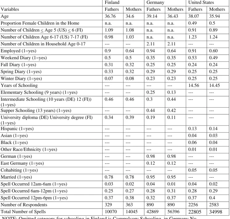
Table A1. Means for Covariates
Finland Germany United States
Variables Fathers Mothers Fathers Mothers Fathers Mothers
Age 36.76 34.6 39.14 36.43 38.07 35.94
Proportion Female Children in the Home n.a. n.a. n.a. n.a. 0.49 0.5 Number of Children < Age 5 (US) < 6 (FI) 1.09 1.08 n.a. n.a. 0.91 0.89 Number of Children Age 6-17 (US) 7-17 (FI) 0.98 1.03 n.a. n.a. 1.23 1.24 Number of Children in Household Age 0-17 --- --- 2.11 2.11 --- ---
Employed (1=yes) 0.9 0.64 0.94 0.64 0.91 0.60
Weekend Diary (1=yes) 0.5 0.5 0.35 0.35 0.53 0.49
Fall Diary (1=yes) 0.31 0.32 0.25 0.25 0.24 0.24
Spring Diary (1=yes) 0.33 0.32 0.29 0.29 0.25 0.25 Winter Diary (1=yes) 0.07 0.08 0.23 0.23 0.25 0.25
Years of Schooling --- --- --- --- 14.56 14.45
Elementary Schooling (9 years) (1=yes) --- --- 0.25 0.13 --- --- Intermediate Schooling (10 years (DE) 12 (FI))
(1=yes)
0.46 0.46 0.3 0.44 --- --- Supper Schooling (13 years) (1=yes) --- --- 0.44 0.42 --- --- University diploma (DE) University degree (FI)
(1=yes)
0.34 0.39 0.19 0.11 --- ---
Hispanic (1=yes) --- --- --- --- 0.13 0.14
Asian (1=yes) --- --- --- --- 0.04 0.03
Black (1=yes) --- --- --- --- 0.06 0.04
Other Race/Ethnicity (1=yes) --- --- --- --- 0.01 0.01
German (1=yes) --- --- 0.98 0.98 --- ---
East Germany (1=yes) --- --- 0.12 0.12 --- ---
Cohabiting (1=yes) --- --- --- --- 0.05 0.05
Married (1=yes) 0.78 0.78 0.95 0.95 --- ---
Spell Occurred 12am-6am (1=yes) 0.03 0.02 0.04 0.01 0.04 0.02 Spell Occurred 6am-12pm (1=yes) 0.25 0.27 0.28 0.31 0.28 0.29 Spell Occurred 12pm-6pm (1=yes) 0.37 0.38 0.32 0.37 0.37 0.4
Number of Respondents 329 363 890 890 2256 2583
Total Number of Spells 10070 14045 42869 56396 22805 34998 NOTE: Omitted category for schooling in Finland is Compulsory Schooling, in Germany No
Schooling. Omitted category for race/ethnicity is White/Non-Hispanic in the United States.
Omitted category for spell time is 6pm-12am, and omitted category for season is diary was in spring in all countries.
Sources: FTUS 1999-2000. GTUS 2001/02, ATUS 2003, not weighted data
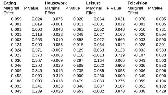
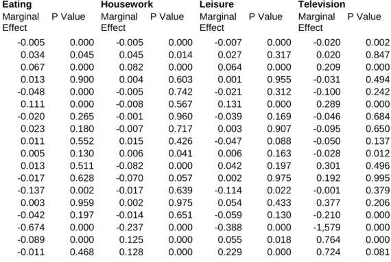
Table A2a. Marginal Effects Associated with the Logistic Regressions Used to Generate Propensity Scores: Finnish fathers (p values in parentheses)
Independent Variables Eating Housework Leisure Television
Marginal Effect
P Value Marginal Effect
P Value Marginal Effect
P Value Marginal Effect
P Value
Respondent’s Age 0.059 0.024 0.076 0.020 0.064 0.021 0.078 0.005
Respondent’s Age squared -0.001 0.019 -0.001 0.011 -0.001 0.012 -0.001 0.005 Number of children age 0-6 0.091 0.000 0.043 0.061 0.052 0.040 -0.010 0.731 Number of children age 7-17 -0.031 0.116 -0.022 0.249 -0.027 0.169 -0.020 0.504 Respondent is employed (1=yes) -0.003 0.953 0.010 0.858 0.022 0.666 -0.033 0.590
Weekend diary (1=yes) 0.124 0.000 0.055 0.015 0.064 0.012 0.028 0.301
Fall diary day (1=yes) -0.024 0.571 -0.067 0.129 -0.063 0.123 -0.033 0.533 Spring diary day (1=yes) -0.023 0.570 -0.063 0.116 -0.013 0.719 -0.107 0.033 Winter diary day (1=yes) 0.036 0.587 -0.069 0.297 0.134 0.066 0.049 0.503 Secondary education (1=yes) -0.046 0.292 -0.029 0.505 0.022 0.606 -0.030 0.553 University digree (1=yes) -0.009 0.849 0.016 0.735 0.085 0.058 -0.006 0.906 Spell occurred between 12am and 6am -0.453 0.000 -0.319 0.000 -0.280 0.000 -0.349 0.000 Spell occurred between 6am and 12pm -0.188 0.000 -0.018 0.479 -0.033 0.275 0.059 0.194 Spell occurred between 12pm and 6pm -0.032 0.241 0.023 0.346 0.037 0.187 0.052 0.192
Married (1=yes) 0.045 0.289 -0.020 0.653 -0.002 0.970 -0.038 0.429
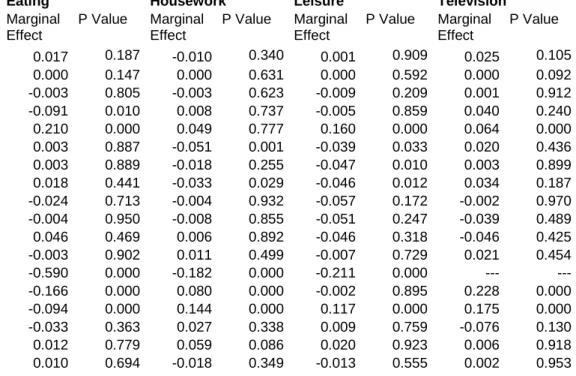
Table A2b. Marginal Effects Associated with the Logistic Regressions Used to Generate Propensity Scores: Finnish mothers (p values in parentheses)
Independent Variables Eating Housework Leisure Television
Marginal Effect
P Value Marginal Effect
P Value Marginal Effect
P Value Marginal Effect
P Value
Respondent’s Age -0.011 0.618 -0.006 0.806 -0.007 0.796 0.004 0.900
Respondent’s Age squared 0.000 0.781 0.000 0.933 0.000 0.907 0.000 0.758 Number of children age 0-6 0.104 0.000 0.085 0.001 0.075 0.004 0.056 0.056 Number of children age 7-17 0.007 0.647 -0.021 0.204 -0.040 0.018 0.003 0.870 Respondent is employed (1=yes) -0.014 0.684 -0.019 0.561 0.024 0.481 -0.038 0.368 Weekend diary (1=yes) 0.036 0.102 -0.005 0.764 0.028 0.231 -0.034 0.189 Fall diary day (1=yes) -0.024 0.528 0.010 0.780 -0.054 0.171 0.003 0.943 Spring diary day (1=yes) -0.002 0.960 -0.013 0.735 -0.030 0.487 -0.020 0.676 Winter diary day (1=yes) 0.002 0.970 -0.025 0.700 -0.002 0.097 0.153 0.025 Secondary education (1=yes) 0.061 0.213 0.047 0.344 0.008 0.876 -0.028 0.607 University digree (1=yes) 0.034 0.499 0.086 0.089 0.002 0.965 0.001 0.985 Spell occurred between 12am and 6am -0.530 0.000 -0.411 0.000 -0.308 0.000 -0.451 0.000 Spell occurred between 6am and 12pm -0.094 0.000 0.014 0.489 0.006 0.816 0.163 0.000 Spell occurred between 12pm and 6pm 0.020 0.391 0.015 0.425 0.078 0.000 0.148 0.000
Married (1=yes) 0.049 0.226 0.059 0.112 0.024 0.544 0.056 0.236
Table A2c. Marginal Effects Associated with the Logistic Regressions Used to Generate Propensity Scores: German fathers (p values in parentheses)
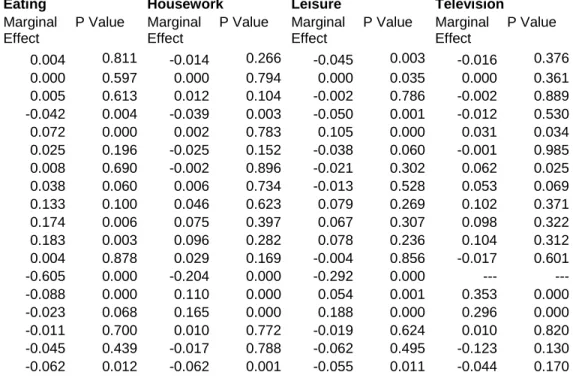
Independent Variables Eating Housework Leisure Television
Marginal Effect
P Value Marginal Effect
P Value Marginal Effect
P Value Marginal Effect
P Value
Respondent’s Age 0.017 0.187 -0.010 0.340 0.001 0.909 0.025 0.105
Respondent’s Age squared 0.000 0.147 0.000 0.631 0.000 0.592 0.000 0.092 Number of children age 0-17 -0.003 0.805 -0.003 0.623 -0.009 0.209 0.001 0.912 Respondent is employed (1=yes) -0.091 0.010 0.008 0.737 -0.005 0.859 0.040 0.240
Weekend diary (1=yes) 0.210 0.000 0.049 0.777 0.160 0.000 0.064 0.000
Fall diary day (1=yes) 0.003 0.887 -0.051 0.001 -0.039 0.033 0.020 0.436 Spring diary day (1=yes) 0.003 0.889 -0.018 0.255 -0.047 0.010 0.003 0.899 Winter diary day (1=yes) 0.018 0.441 -0.033 0.029 -0.046 0.012 0.034 0.187 Elementary Schooling (1=yes) -0.024 0.713 -0.004 0.932 -0.057 0.172 -0.002 0.970 Intermediate Schooling (1=yes) -0.004 0.950 -0.008 0.855 -0.051 0.247 -0.039 0.489 Supper Schooling (1=yes) 0.046 0.469 0.006 0.892 -0.046 0.318 -0.046 0.425 University diploma (1=yes) -0.003 0.902 0.011 0.499 -0.007 0.729 0.021 0.454 Spell occurred between 12am and 6am -0.590 0.000 -0.182 0.000 -0.211 0.000 --- --- Spell occurred between 6am and 12pm -0.166 0.000 0.080 0.000 -0.002 0.895 0.228 0.000 Spell occurred between 12pm and 6pm -0.094 0.000 0.144 0.000 0.117 0.000 0.175 0.000
Married (1=yes) -0.033 0.363 0.027 0.338 0.009 0.759 -0.076 0.130
German (1=yes) 0.012 0.779 0.059 0.086 0.020 0.923 0.006 0.918
East German (1=yes) 0.010 0.694 -0.018 0.349 -0.013 0.555 0.002 0.953
Table A2d. Marginal Effects Associated with the Logistic Regressions Used to Generate Propensity Scores: German mothers (p values in parentheses)
Independent Variables Eating Housework Leisure Television
Marginal Effect
P Value Marginal Effect
P Value Marginal Effect
P Value Marginal Effect
P Value
Respondent’s Age 0.004 0.811 -0.014 0.266 -0.045 0.003 -0.016 0.376
Respondent’s Age squared 0.000 0.597 0.000 0.794 0.000 0.035 0.000 0.361 Number of children age 0-17 0.005 0.613 0.012 0.104 -0.002 0.786 -0.002 0.889 Respondent is employed (1=yes) -0.042 0.004 -0.039 0.003 -0.050 0.001 -0.012 0.530
Weekend diary (1=yes) 0.072 0.000 0.002 0.783 0.105 0.000 0.031 0.034
Fall diary day (1=yes) 0.025 0.196 -0.025 0.152 -0.038 0.060 -0.001 0.985 Spring diary day (1=yes) 0.008 0.690 -0.002 0.896 -0.021 0.302 0.062 0.025 Winter diary day (1=yes) 0.038 0.060 0.006 0.734 -0.013 0.528 0.053 0.069 Elementary Schooling (1=yes) 0.133 0.100 0.046 0.623 0.079 0.269 0.102 0.371 Intermediate Schooling (1=yes) 0.174 0.006 0.075 0.397 0.067 0.307 0.098 0.322 Supper Schooling (1=yes) 0.183 0.003 0.096 0.282 0.078 0.236 0.104 0.312 University diploma (1=yes) 0.004 0.878 0.029 0.169 -0.004 0.856 -0.017 0.601 Spell occurred between 12am and 6am -0.605 0.000 -0.204 0.000 -0.292 0.000 --- --- Spell occurred between 6am and 12pm -0.088 0.000 0.110 0.000 0.054 0.001 0.353 0.000 Spell occurred between 12pm and 6pm -0.023 0.068 0.165 0.000 0.188 0.000 0.296 0.000
Married (1=yes) -0.011 0.700 0.010 0.772 -0.019 0.624 0.010 0.820
German (1=yes) -0.045 0.439 -0.017 0.788 -0.062 0.495 -0.123 0.130
East German (1=yes) -0.062 0.012 -0.062 0.001 -0.055 0.011 -0.044 0.170