7 Turbulence Spectra
7.1 Introduction to spectral analysis
The understanding of turbulence as being a superposition of ‘eddies’ of all sizes has implicitly been used in many previous sections. In describing turbulence in a statistical approach (Chapter 3) we have explicitly given up the idea to ‘trace each fluid element’ but rather attempted to describe its overall properties. However, for the understanding of turbulence, its production, development and decay it is important to know which ‘eddies’ contribute to what property of the flow field. The spectral decomposition of turbulence fields can give us exactly this information. In expressing a given signal as a superposition of contributions from all possible frequencies or wave lengths as in the Fourier decomposition1 – hence in constructing a power spectrum of the signal – we can investigate which fluctuations contribute to what extent to the (co-)variance of the original signal.
Power spectra may be constructed in the space and the time domain, respectively. The former corresponds to what we are mainly interested in because it addresses questions like ‘Eddies of what size contribute how to the total variance?’; ‘Are these eddies round like a soccer ball or rather elliptic like an (American) football?’; ‘How do eddy length scales correspond to ABL length scales like the ABL height?’; etc. However, spectra in the space domain are difficult to obtain because they require either a very fine resolution in numerical models or many, many instruments to be deployed in the field.
Spectra in the time (frequency) domain, on the other hand, can already be obtained from one single instrument measuring at high enough pace. Most commonly, therefore, spectral information is derived in the time domain and then transformed into the space domain by invoking Taylor’s hypothesis (see Section 3.2). Equation (3.15) gives the relation between the wavelength,
€
λ, and the frequency,
€
f, using Taylor’s hypothesis.
In this Chapter we do not concentrate on time series analysis in the technical sense. For this we refer to more specialized texts (Priestley, 1981). We closely follow Kaimal and Finnigan (1994) to summarize the essentials for boundary layer spectra. All the formulae are expressed in one-dimensional form and with the longitudinal component as an example.
The auto-covariance function in the space domain for a variable
€
a under horizontally homogeneous conditions reads
€
Ca(r1)=a'(x1)⋅a'(x1+r1). (7.1) Similarly, in the time domain (cf. equation 3.9) we have, when using Taylor’s hypothesis (
€
r1=u 1τ)
1 In this chapter we indeed use the Fourier transform as it is the most commonly used approach. Other approaches such as the ‘wavelet transform’ employ a targeted function rather than sine and cosine functions to decompose the signal and are used to detect specific structures in a turbulent flow.
- 2 -
€
Ca(τ)=a'(t)⋅a'(t+τ). (7.2)
The one-dimensional, two-sided power spectra are obtained from applying a Fourier transform to the auto-covariance functions:
€
F ) a(κ1)=:F
{
Ca(r1)}
= 21π Ca(r1)e−iκ1r1−∞
∞
∫ dr1. (7.3)
€
S ) a(ω)=:F
{
Ca(τ)}
=2π1 Ca(τ)e−iωτ−∞
∞
∫ dτ. (7.4)
Here,
€
κ1 is the longitudinal component of the wave number,
€
κ1=2πf /u 1,
€
f the natural frequency ([
€
f] = s-1) and
€
ω =2πfis the cyclic frequency. Throughout the following, ‘F’ is employed for the spectral density [function] in the space domain and ‘S’ for that in the time domain. The ‘hat’ (as in
€
F ) ) denotes two- sided spectrum. Taylor’s hypothesis yields
€
F ) a(κ1)=u 1)
S a(ω). (7.5)
The backward transforms of (7.3) and (7.4) read2
€
Ca(r1)=F-1 ) F a(κ1)
{ }
= F ) a(κ1)eiκ1r1−∞
∞
∫ dκ1. (7.6)
€
Ca(τ)=F-1 ) S a(ω)
{ }
= S ) a(ω)eiωτ−∞
∞
∫ dω. (7.7)
For the relation between the two-sided (symbol with a ‘hat’) and one-sided (symbol without ‘hat’) spectra in the time-frequency domain we require that both spectral representations integrate to the total variance of the variable under consideration (Priestley 1981)
€
Sa(f)
o
∞
∫ df =σa2 = ) S a(ω)
−∞
∞
∫ dω. (7.8)
Noting further that
€
S ) a(ω) is an even function we have (Kaimal and Finnigan, 1994)
€
Sa(f) = 2)
S (f) = 4π)
S a(ω) (7.9)
In practice, time series are measured (or ‘logged’ from the output of numerical model) as
€
X(t)= x(t), - T≤t≤T 0 otherwise
(7.10)
The Fourier pair to (7.10) is
€
XT(t)= )
G T(ω)eiωτ
−∞
∞
∫ dω (7.11)
2 Note that the normalisation convention here is different from some mathematical texts, where both the forward and backward transforms are attributed with
€
1 2π.
€
G ) T(ω)= 1
2π XT(t)e−iωt
−∞
∞
∫ dt = 1
2π X(t)e−iωt
−T T
∫ dt. (7.12)
The contribution to the total energy of
€
XT(t), from the components between
€
ω and
€
ω+Δω is
€
G ) (ω)2dω. Noting that power is energy per time the contribution to the total power of
€
XT(t) as contributed by the components with frequencies between
€
ω and
€
ω+Δω is
€
lim(T → ∞) )
G (ω)2dω/ 2T. The spectral power is estimated from the time series according to
€
S ) x(ω)=lim(T → ∞)E
G ) (ω)2dω 2T
(7.13)
where
€
E
{ }
denotes the expected value. Thus from€
XT(t) a Fourier transform yields
€
G ) T(ω), from which
€
G(f) and finally
€
Sx(f) can be estimated.
We finally note that as another measure of the turbulence structure, the so- called structure function may be useful. It is defined, e.g. in the time domain
€
Da(τ)=
(
a'(t)−a'(t+τ))
2. (7.14)Under stationary conditions the structure function is related to the auto covariance function through
€
Da(τ)=2
(
σa2−Ca(τ))
, (7.15)and through the Fourier transform also to the spectral density. Which of these measures to analyze the turbulence structure is most appropriate depends on the application and availability of data.
When considering cospectra, i.e. if we are interested in how the covariances are spectrally distributed, we have to start from the covariance function rather than from the auto-covariance function (7.1)
€
Cab(r1)=a'(x1)⋅b'(x1+r1). (7.16) This function is – opposite to the auto-covariance function – not an even function, because in general
€
a'(x1)⋅b'(x1+r1)≠a'(x1+r1)⋅b'(x1). Its Fourier transform therefore has a real and an imaginary part, i.e. for the two-sided total cospectrum,
€
F ) ab, we obtain
€
F ) ab(κ1)= 1
2π Cab(r1)e−iκ1r1
−∞
∞∫ dr1= )
C oab(κ1)−i)
Q (κ1). (7.17) We formally split up the covariance function according to
€
Cab(r1)=Gab(r1)+Uab(r1), (7.18)
- 4 - where
€
Gab is the even part and
€
Uab the odd part. The cospectrum,
€
C o) ab, and the quadrature spectrum,
€
P ) ab, then correspond to the Fourier transforms
€
C o) ab(κ1)= 1
2π Gab(r1)e−iκ1r1
−∞
∞
∫ dr1. (7.19)
€
Q ) ab(κ1)= i
2π Uab(r1)e−iκ1r1
−∞
∞∫ dr1. (7.20)
The cospectrum contains the information on how the covariances are spectrally distributed since
€
a'b'=Cab(0)= ) C oab(κ1)
−∞
∞
∫ dκ1 (7.21)
and in particular since the odd part of the auto-covariance function,
€
Uab, has no contribution to
€
Cab(0). The quadrature spectum, on the other hand, contains the information on the phase shift between the variables
€
a and
€
b.
7.2 Energy Cascade
The Russian scientist Kolmogorov (1941) introduced the equilibrium theory of turbulence with the corresponding picture of an idealized spectrum. Its basis is that he noted that eddies containing most of the energy are those at the small wave numbers (large wave length), which were produced by instability of the mean flow. They are thus highly anisotropic and represent the configuration of the boundary conditions. In the ABL this is the bounding of the flow by the surface (friction, energy exchange). These large eddies themselves are prone to instability due to, e.g., the shear stress of the mean flow acting on them. Hence they break into smaller eddies and this process continues until the eddies are so small that they begin to be affected by viscous forces. Finally then, dissipation transforms the turbulent kinetic energy into heat at the smallest eddy sizes. The picture of eddies breaking up into smaller ones is known as the energy cascade due to the similarity to a (water) cascade. It was very nicely summarized by L.F. Richardson in a poem
Big whirls have little whirls That feed on their velocity
And little whirls have lesser whirls
And so on to viscosity (in the molecular sense)
Figure 7.1 displays the idealized energy spectrum corresponding to this picture of an energy cascade. The energy containing range, where the input from the mean flow occurs, is characterised by length scales from 10m to 1000m and time scales 10 to 1000s. The maximum energy occurs at a wavenumber that is inversely proportional to an integral length scale, which in turn is related to the integral time scale (eq. 3.29) through Taylor’s
hypothesis,
€
Λa =u 1Ta. In this wavenumber range the magnitude of the spectral power is dependent on the overall characteristics of the flow and hence scale with parameters such as
€
u*, u , L, zi.
Figure 7.1 Idealized spectrum according to the hypotheses of Kolmogorov. The numbered three ranges correpond to the energy containing range (1), the Inertial Subrange (2) and the Dissipation range (3).
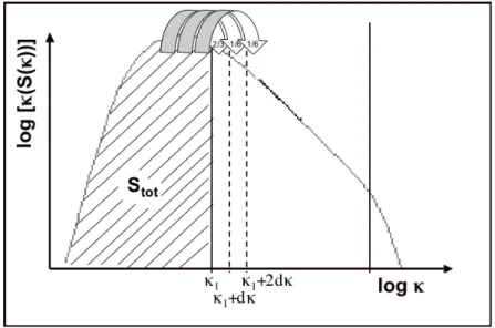
The very ‘cascade range’ of the spectrum is called inertial subrange and it is characterised by the fact that turbulent energy is neither produced nor dissipated but only transported through. For this inertial subrange Kolmogorov was therefore able to make universal predictions (see Section 7.3) since its shape and characteristics do not depend on external parameters. Based on sophisticated models it has been estimated how the transfer of energy occurs in the ‘cascade’. If we consider the energy of all eddies with wave number smaller than
€
κi in Fig. 7.2, about two thirds of their energy will be ‘given’ to eddies with wave numbers between
€
κi and
€
κi +dκ (i.e. the ‘next smaller eddies’), one sixth goes to eddies between
€
κi +dκ and
€
κi +2dκ and the remaining one sixth goes to even smaller eddies (REF??).
In the dissipation range finally, turbulent energy is transformed into heat by the action of viscous forces. It may be useful to recall that the energy thereby released is by no means relevant (as judged by magnitude) to the heat budget of a turbulent flow. Again Kolmogorov’s theory of universal equilibrium makes a prediction at which scales the transition from the inertial subrange to the dissipation range occurs.
- 6 -
7.3 Kolmogorov Hypotheses
The first Hypothesis, which was central in Kolmogorov’s theory of universal equilibrium concerns the inertial subrange. It basically states that there must be a range in the turbulence spectrum in which the turbulence can be assumed to be locally isotropic. ‘Local’ in this context refers to the location in the spectrum not in space. With his first hypothesis Kolmogorov therefore demands the existence of an inertial subrange (IS) if eddies of a particular size (range) can be assumed to be isotropic. In sketching the energy cascade we have noted that even in this range energy is transported from larger to smaller eddies through their instability, which in turn was attributed (inter alia) to the action of deformation through the mean flow. Hence this local isotropy can only be meant in a statistical sense.
Figure 7.2 Sketch of energy transfer in the ‘cascade’. Adopted from (missing REF!).
If the turbulence is locally isotropic the spectral density (in the IS) must not depend on energy production (i.e., on external parameters like
€
u*, u , L, zi), nor on the viscosity (which determines the dissipation). Therefore
€
F(κ1)=f
(
κ1, ε)
(7.22)for the one-dimensional spectral density. One may wonder why
€
ε is in the list of attributes in (7.22) even if dissipation is not considered an important process in the IS. This is due to the fact that – if the IS is viewed as a ‘tube’
through which the energy is transported from the energy containing to the dissipation range (cf. the ‘cascade’) –
€
ε stands for the rate at which it finally can be dissipated and therefore also characterises the ‘flow rate through the tube’. Dimensional analysis for (7.22) readily yields
€
F(κ1)=α1κ1−5 / 3
ε2 / 3, (7.23)
where
€
α1 is the (one dimensional) proportionality factor known as the Kolmogorov constant. Experimental evidence suggests that
€
α1≈0.55 (i.e., in the range between 0.5 and 0.6) and for the three-dimensional Kolmogorov constant,
€
α ≈1.5. A further consequence of local isotropy, which is mathematically difficult to comprehend (see Panofsky and Dutton, 1984) and therefore not explicitly worked out here, is that
€
α2 =α3 =4 / 3α1 and hence
€
Fu
2(κ2)=Fu
3(κ3)= 4 3Fu
1(κ1), (7.24)
since
€
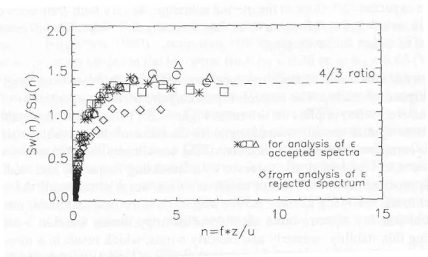
ε is the same for all three coordinate directions. Due to the very general (‘universal’) assumptions leading to (7.23) and (7.24) they also constitute a comprehensive test for an IS in a spectral analysis of a time series. Indeed the ‘minus five thirds slope’ is very often found - even for time series that were obtained in a location where we would not necessarily expect ‘local equilibrium’ to prevail (between buildings, say, in a street canyon – see section 8.2). The more stringent test on IS behaviour is the ratio of spectral densities (7.24) and often the IS has to be constrained by inspecting this ratio (Fig. 7.3).
Figure 7.3 IS test on 4/3 ratio. Ratio of spectral density as a function f non- dimensional frequency. From Weiss (2002).
In a similar manner as for the velocity spectra the IS form of the temperature spectrum can be determined (Kaimal and Finnigan (1994)
€
Fθ(κ1)=β1κ1−5 / 3
Nθε−1/ 3, (7.25)
where
€
Nθ is the dissipation rate for
€
σθ / 2 and
€
β1 ≈0.8 is, again, a universal constant. Kaimal and Finnigan (1994) note that (7.25) apparently is suitable for other scalars.
- 8 -
Local isotropy would, in fact, imply that the co-spectra should completely vanish in the IS (the velocity field being independent of rotation). They are indeed found to be very low with a much faster roll-off (proportional to
€
κ−7 / 3) for the IS (Wyngaard and Cote 1972).
The second of Kolmogorov’s hypotheses concerns the so-called micro scales.
It can be summarized as ‘at the high-frequency end of the inertial subrange it is only the dissipation rate of TKE,
€
ε, and the (molecular) viscosity,
€
υ, which determine the spectral density’. From this hypothesis the time, length and velocity scales can be determined that characterise the dissipation range.
Dimensional analysis yields
€
ηK = ν3 ε
1/ 4
length scale (7.26)
€
τK = ν ε
1/ 2
time scale (7.27)
€
uK =
( )
νε 1/ 4 velocity scale. (7.28)Inserting typical values in (7.26) to (7.28) we find
€
ηK =O(10−3m),
€
τK =O(10−1s) and
€
uK =O(10−2ms−1). Thus the smallest turbulent eddies are on the order of millimetres and any numerical model attempting to resolve these will have to use a very fine grid and correspondingly small time steps.
7.4 Spectra and Co-spectra
Recalling (7.8) we are tempted to display spectral information in a linear fashion so that the area under the spectral curve corresponds to the variance of the variable under consideration. However, in this representation not much can be seen (see Stull, 1988, his Fig. 8.9). It has therefore become standard to represent
€
fSi(f) vs.
€
f in a double logarithmic frame since in this representation also the variance corresponds to the area under the spectral curve (Stull 1988).
7.4.1 Surface Layer spectra
Monin-Obukhov scaling can be used to represent spectral curves in the SL.
For this we start from (7.23) and recall that, in fact, we would like to represent our spectral curves as
€
fSi(f). We start from Taylor’s hypothesis for the two- sided spectra (eq. 7.5) and use (7.9) for the time domain (
€
S ) a(ω)=Sa(f)/4π) as well as for the space domain (
€
F ) a(κ1)=Fa(κ1)/2). Therefore
€
1
2Fa(κ1)= u 1
4πSa(f), (7.29)
which, upon multiplication by (
€
4πf /u ) becomes
€
2πf
u Fa(κ1)=fSa(f)=κ1Fa(κ1). (7.30)
We may therefore use Kolomogorov’s hypothesis on the IS (7.23) as a starting point even in the frequency domain:
€
fS(f)=α1 2πf u 1
−2 / 3
ε2 / 3. (7.31)
Introducing a non-dimensional frequency,
€
n=fx3/u 1 and rearranging yields
€
fS(f)= α1 (2π)2 / 3
(εx3)2 / 3n−2 / 3. (7.32)
Now, the non-dimensional function for the dissipation rate,
€
Φε =εkx3/u*3 (see eq. 6.17) is introduced and, upon further rearrangement and insertion of the numerical values we obtain for the three velocity spectra
€
fSu
1(f)
u*2Φε2 / 3 =0.3n−2 / 3, fSu
2,u3(f)
u*2Φε2 / 3 =0.4n−2 / 3. (7.33)
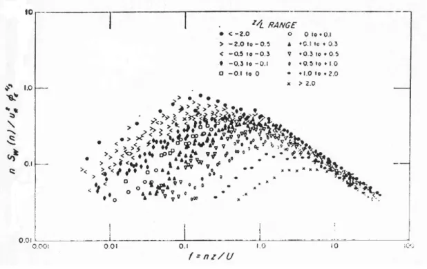
In this representation due to using the IS prediction according to (7.23), all the spectra are expected to collapse to one curve in the inertial subrange. Indeed, Fig. 7.4 shows this behaviour in the spectra of the famous ‘Kansas experiments’ over almost ideally flat and homogeneous terrain (Kaimal et al.
1972) – and has been documented in numerous examples ever since. The stability dependence is represented through
€
Φε(x3/L), i.e. the requirement according to MOST that all the variables be only a function of
€
x3/L. We readily observe that for the most stable stratification only the smallest eddies are present (and dominant) while with increasing instability eddy sizes grow.
Figure 7.4 SL spectra (example w) from Kansas (Kaimal et al 1972)
- 10 -
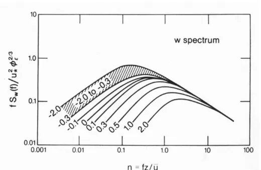
Based on eq. (7.33) curves (parameterizations) can be fitted through the data to describe their overall behaviour. Rather than explicitly formulate these, we refer to Kaimal and Finnigan (1994) for a comprehensive overview and show their summarizing figures (Fig. 7.5).
Figure 7.5 Non-dimensional SL spectra for different ranges of stability. From Kaimal and Finnigan (1994)
In a similar fashion as for the velocity spectra above, SL scaling can be used to derive non-dimensional forms for the temperature spectra
€
fSθ(f)
θ*2ΦNΦε−1/ 3 =0.43n−2 / 3, (7.34)
where
€
ΦN is the non-dimensional function for
€
Nθ according to MOST (see Kaimal and Finnigan 1994). A parameterized, again from Kaimal and Finnigan (1994) is reproduced in Fig. 7.6. The co-spectra in the SL ‘suffer’ to some extent from the success of the energy and temperature spectra, which were based Kolmogorov’s IS predictions. According to the requirement of local isotropy co-spectral density should vanish in the IS. In fact, it is only found to drop off faster than the energy and temperature spectra. Figure 7.7 shows that indeed the co-spectra exhibit a spectral slope in the IS according to
€
fCoab(f)∝n−4 / 3. (7.35)
However, it can be seen that the velocity co-spectrum (
€
u1u3) attains this behaviour at lower frequency than the
€
u3θ co-spectrum. Still, the experimental evidence suggests co-spectral curves can be parameterized in the SL based on universal functions of stability (Kaimal and Finnigan 1994).
- 12 -
Figure 7.6 Parameterized temperature spectra for the SL. Different stabilities as indicated. From Kaimal and Finnigan (1994).
Figure 7.7 Parameterized co-spectra for the SL. Different stabilities as indicated.
From Kaimal and Finnigan (1994).
7.4.2 Mixed Layer spectra
In the ML the scaling variables are
€
w* and
€
zi (Section 4.5.3), and correspondingly the scaling approach for the IS is modified. Introducing a new non-dimensional frequency
€
ni =fzi /u 1 and the ratio of dissipation and buoyant
production in the TKE equation (6.6),
€
Ψε =ε/(g/θ )(u'3θ')o, leads to a formulation for the ML spectra similar to those in the SL:
€
fSu
1(f)
w*2Ψε2 / 3 =0.16ni−2 / 3, fSu
2,u3(f)
w*2Ψε2 / 3 =0.21ni−2 / 3. (7.36)
Figure 7.8 shows idealized spectral curves for various ranges of
€
x3/zi indicating that ML spectra do not change the position of the spectral peak with height – which is clear since none of the scaling variables changes with height in the ML.
Under convective conditions the wavelength of the spectral peaks for
€
u1, u2 and u3 vary according to (Kaimal and Finnigan 1994)
€
λmax,u1 =λmax,u2 =1.5zi, 0.01zi <x3<zi. (7.37)
€
λmax,u3 = 5.9x3, - L<x3 <0.1zi 1.8zi(1−e−4x3/zi−0.0003e8x3/zi), 0.1zi ≤x3 ≤zi
(7.38)
Especially the relation between the spectral peak of the horizontal spectra and the ML height, which is valid in a quite large height range, may be utilized to infer
€
zi from the reading of single instrument relatively close to the surface.
Figure 7.8 ML spectra for different non—dimensional height ranges. From Kaimal and Finnigan (1994).
- 14 - 7.4.3 Spectra in the Local Scaling Layer
In stable stratification spectral information is relatively scarce outside the surface layer. Forrer (1999) has investigated turbulence characteristics over a nearly flat and extensively homogeneous snow and ice-covered surface over the Greenland ice sheet. As a scaling approach he used a parameterization by Olesen et al. (1984) for the stable SL3, but – in the light of Local Scaling – replaced
€
u* and
€
L by their local counterparts
€
fSu
1(f)
−τ = 96(n Φm) 1+321(n Φm)5 / 3
(Φm
Φε )2 / 3 (7.39)
€
fSu
2(f)
−τ = 13(n Φm) 1+32(n Φm)5 / 3
(Φm
Φε )2 / 3 (7.40)
€
fSu
3(f)
−τ = 4.5(n Φm) 1+11(n Φm)5 / 3
(Φm
Φε )2 / 3. (7.41)
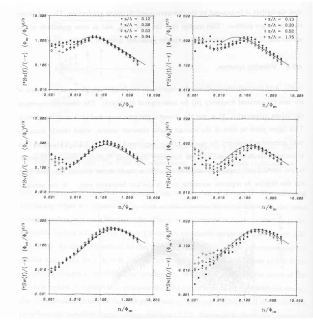
Figure 7.9 shows the spectral curves from two different levels on a tower and for different stability classes to closely collapse to one curve – as predicted by the model of Olesen et al (1984). Note that in this approach the non- dimensional frequency is scaled with the non-dimensional wind shear, i.e.
€
n/Φm. Note also that the correspondence between stability classes ceases at low frequency where wave activity may have played a role.
3 Note that the numerical factors in (3.39) to (3.41) are slightly different than those proposed by Olesen et al (1984).
Figure 7.9 Normalized spectra for the SBL. Longitudinal (upper panels), lateral (middle panels) and vertical (lower panels velocity components, from observations at 10m above ground (left) and 30m above ground (right) at ‘Swiss camp’ on the Greenland Ice Sheet. The solid lines correspond to eqs (7.39) to (7.41) respectively. From Forrer (1999).
The spectra of Fig. 7.9 stem from observations at
€
x3 =10m and
€
x3 =30m, respectively and thus might easily thought to be from within the SL. Still, the continuously stable BL over an ice sheet can be quite shallow so that even these levels may lie well in the ‘middle’ of the SBL. The katabatic wind4, which is a characteristic flow phenomenon in such an environment, very often exhibits a distinct maximum, the height of which may be employed as a length
4 The katabatic wind is a drainage flow that occurs over sloped surfaces under stable stratification through the combined action of gravity and (horizontal) density differences between near-surface positions and those farther away from the surface. See Fig. 8.11 for an illustration. This type of flow is simply called ‘slope flow’ over limited (in space) slopes, while over sometimes largely extended slopes such as on an ice sheet, they are referred to as ‘katabatic wind’. In the latter case they can be substantial in magnitude (some 10ms-1) and quite steady.
- 16 -
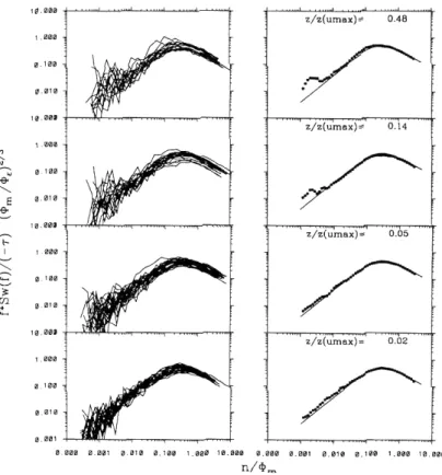
scale. Figure 7.10 shows the spectra grouped into different classes of
€
x3/x3,umax, where
€
x3,umax corresponds to the height of the wind maximum.
Except for the low frequency part, especially in the longitudinal and lateral velocity components, eqs. (7.39) to (7.41), i.e. the model of Olesen et al (1984) in its Local Scaling form, appear to describe the spectra extremely well – at least up to the middle of the SBL.
Figure 7.10a Spectra of the vertical velocity component for four non-dimensional heights in the SBL during conditions of katabatic wind. The height is scaled with the height of the wind maximum (as surrogate for the SBL height). Solid line represents eq. (7.41). From Forrer (1999).
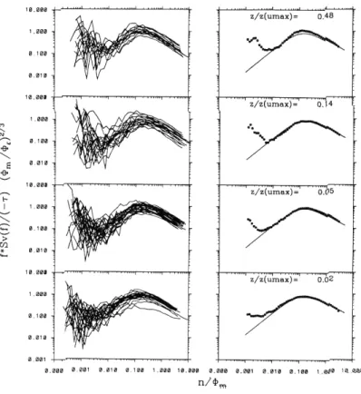
Figure 7.10b As Fig. 7.10a, but for lateral velocity component. Solid line represents eq. (7.40). From Forrer (1999).
Figure 7.10b As Fig. 7.10a, but for lateral velocity component. Solid line represents eq. (7.40). From Forrer (1999).
- 18 -
7.5 Application of Spectral Information
Clearly, the foremost goal of spectral analysis lies in the investigation of the turbulence structure in particular flow. The existence of a true inertial sublayer (validity of 7.23 a n d 7.24) indicates that a minimum condition for an equilibrium flow (at least at high frequency) is fulfilled. Raupach et al (1991) have noted that the inertial sublayer is the spectral equivalent to an inertial sublayer, which latter is the true matching layer, i.e. the ‘surface layer’ (see discussion in connection to Fig. 1.3). In studies concerned with turbulent exchange within and above canopies (plants, forests, buildings) failure of one (or both) of the IS conditions often can help to interpret the data (e.g., Rotach 1995) and to quantify the (vertical) extension of the Roughness sublayer (see Section 8.2). The measured (or parameterized) spectral curves yield furthermore information on spatial/temporal scales of the flow. For example the frequency (wavelength) of the spectral peak, i.e. the ‘size’ of the dominant eddies has found to be related to the ABL height through (7.37) and (7.38) for spectra from the ML (Kaimal and Finnigan 1994). As mentioned above, the ML height, which requires remote sensing or profile instrumentation to be observed may thus be inferred from a ‘simple’ near-surface measurement of a turbulence spectrum. Similarly, the spectra in spatially constrained flows (in a valley, say, or within a street canyon) often indicate to what extent and how the turbulence is determined or possibly limited through the spatial scales involved (e.g., Rotach 1995).
In the following a limited number of practical applications of spectral information – beyond the examination of turbulence structures – is summarized briefly in order to give some (by far not exhaustive) examples.
Determination of dissipation rate for TKE The dissipation rate of TKE,
€
ε, is very difficult to determine experimentally.
The only practical approach available today consists of using the spectral information from the IS and the Kolomogorov prediction (e.g., eq. 7.30 for the SL). Identifying the spectral range of the IS (Fig. 7.3) and using the spectral density allows then to solve (7.30) for
€
ε and hence estimating the dissipation rate. From the above discussion concerning the equivalence of inertial sublayer and inertial subrange it becomes clear that the application of this method in, e.g. the roughness sublayer (Section 8.2) is at least questionable.
Still, due to the lack of other experimental means to determine
€
ε, it is usually employed even there.
Inertial dissipation method for turbulent fluxes
Turbulent fluxes can nowadays easily be measured using fast enough instrumentation. However, this is only true if the platform, on which the instrument is mounted, is at rest. For instruments on moving platforms (ships, say, to determine turbulent exchange over the sea or airborne instrumentation) it is often difficult to distinguish between the movement of the platform itself and the turbulence that is aimed to be observed. Again, the IS behaviour of the spectrum may be used then to determine the surface fluxes
of momentum and sensible heat (Taylor 1961; Fairall and Larsen 1986). For this, eq. (7.32) and the equivalent for temperature spectra (Kaimal and Finnigan 1994) can be employed. The stability can be inferred from, e.g., the (Gradient) Richardson number (6.13) and an estimate can be made for
€
x3/L through iteration. Hence,
€
Φε can be determined using a parameterization according to MOST5. Thus (7.32) can be solved for
€
u* (and the equivalent for
€
θ*, i.e. the surface heat flux from the temperature spectrum).
Structure function
The structure function (7.14) has many practical applications, such as in the interpretation of remote sensing data6 or in the assimilation of data into numerical models. Parameterized spectra within the various layers of the ABL can be used to find appropriate values for the structure function in operational applications. Figure 7.11 shows typical vertical profiles of the so-called structure parameter, which corresponds to the spatial equivalent to (7.15), but scaled with the separating distance to the 2/3 power,
€
r12 / 3 (Kaimal and Finnigan 1994).
Figure 7.11 Vertical profiles of the normalized structure parameters in the CBL.
From Kaimal and Finigan (1994).
5 Note that often the non-dimensional form of the TKE equation (6.17) is used to represent
€
Φε in terms of the non-dimensional wind-shear, the stability parameter and sometimes even the (non-dimensional) transport and pressure correlation terms.
6 For example SODAR: The intensity or amplitude of the returned energy is proportional to the structure parameter for temperature,
€
CT2, which, in turn, is related to the thermal structure and stability of the atmosphere. In particular,
€
CT2 has characteristic patterns at any interface between air masses of different temperatures.
- 20 -
References Chapter 7
Fairall, C. W., and Larsen S. E.: 1986, Inertial dissipation methods and turbulent fluxes at the air-ocean interface. Boundary-Layer Meteorol., 34, 287-301.
Kaimal J.C., Wyngaard J.C., Izumi Y. and Coté, O.R.: 1972, Spectral characteristics of surface layer turbulence, Quart J Roy Meteorol Soc, 98, 563-589.
Kaimal, J.C. and Finnigan, J. J.: 1994, Atmospheric Boundary Layer Flows, Oxford University Press, New York, 289pp.
Kolmogorov, A.N.: 1941, The local structure of turbulence in an incompressible fluid for very large Reynolds numbers, Dok Akad Nauk SSSR, 30, 301-305; and 32, 16-18.
Panofsky H.A. and Dutton J.A.: 1984, Atmospheric Turbulence, John Wiley & Sons, New York, 397pp.
Olesen H.R., Larsen S.E. and Højstrup J.: 1984, Modeling velocity spectra in the lower part of the planetary boundary layer, Boundary-Layer Meteorol, 29, 285-312.
Priestley M.B.: 1981, Spectral Analysis and Time Series, academic Press, London, 890pp.
Raupach M. R., Antonia R. A., and Rajagopalan S.: 1991, ‘Rough-Wall Turbulent Boundary Layers’, Appl. Mech. Rev. 44, 1–25.
Rotach M.W.: 1995, 'Profiles of Turbulence Statistics in and Above an Urban Street Canyon', Atmospheric Environ., 29, 1473-1486.
Stull RB: 1988, An introduction to Boundary Layer Meteorology, Kluwer, Dordrecht, 666pp.
Taylor, R.J: 1961, A new approach to the measurement of turbulent fluxes in the lower atmosphere, J Fluid Mech, 10, 449-458.
Weiss A: (2002), ‘Determination of stratification and turbulence of the atmospheric surface layer for different types of terrain by optical scintillometry’, ETH Dissertation #14514, 148pp
Wyngaard J.C. and Coté O.R.: 1972, Cospectal similarity in the atmospheric surface layer, Quart J Roy Meteorol Soc, 98, 590-603.