Comparing Bayesian Models of Annotation

Comparing Bayesian Models of Annotation

Silviu Paun

Bob Carpenter

Jon Chamberlain

Dirk Hovy

Udo Kruschwitz

Massimo Poesio

1

School of Electronic Engineering and Computer Science, Queen Mary University of London

2

Department of Statistics, Columbia University

3

School of Computer Science and Electronic Engineering, University of Essex

4

Department of Marketing, Bocconi University

Abstract

The analysis of crowdsourced annotations in natural language processing is con- cerned with identifying (1) gold standard labels, (2) annotator accuracies and biases, and (3) item difficulties and error patterns.

Traditionally, majority voting was used for 1, and coefficients of agreement for 2 and 3. Lately, model-based analysis of corpus annotations have proven better at all three tasks. But there has been relatively little work comparing them on the same datasets.

This paper aims to fill this gap by ana- lyzing six models of annotation, covering different approaches to annotator ability, item difficulty, and parameter pooling (tying) across annotators and items. We evaluate these models along four aspects:

comparison to gold labels, predictive accu- racy for new annotations, annotator char- acterization, and item difficulty, using four datasets with varying degrees of noise in the form of random (spammy) annotators. We conclude with guidelines for model selec- tion, application, and implementation.

1 Introduction

The standard methodology for analyzing crowd- sourced data in NLP is based on majority vot- ing (selecting the label chosen by the majority of coders) and inter-annotator coefficients of agree- ment, such as Cohen’s κ (Artstein and Poesio, 2008). However, aggregation by majority vote implicitly assumes equal expertise among the annotators. This assumption, though, has been re- peatedly shown to be false in annotation prac- tice (Poesio and Artstein, 2005; Passonneau and Carpenter, 2014; Plank et al., 2014b). Chance- adjusted coefficients of agreement also have many shortcomings—for example, agreements in mis- take, overly large chance-agreement in datasets with skewed classes, or no annotator bias correc- tion (Feinstein and Cicchetti, 1990; Passonneau and Carpenter, 2014).

Research suggests that models of annotation can solve these problems of standard practices when applied to crowdsourcing (Dawid and Skene, 1979; Smyth et al., 1995; Raykar et al., 2010;

Hovy et al., 2013; Passonneau and Carpenter, 2014). Such probabilistic approaches allow us to characterize the accuracy of the annotators and correct for their bias, as well as account- ing for item-level effects. They have been shown to perform better than non-probabilistic alterna- tives based on heuristic analysis or adjudication (Quoc Viet Hung et al., 2013). But even though a large number of such models has been proposed (Carpenter, 2008; Whitehill et al., 2009; Raykar et al., 2010; Hovy et al., 2013; Simpson et al., 2013; Passonneau and Carpenter, 2014; Felt et al., 2015a; Kamar et al., 2015; Moreno et al., 2015, in- ter alia), it is not immediately obvious to potential users how these models differ or, in fact, how they should be applied at all. To our knowledge, the literature comparing models of annotation is lim- ited, focused exclusively on synthetic data (Quoc Viet Hung et al., 2013) or using publicly available implementations that constrain the experiments al- most exclusively to binary annotations (Sheshadri and Lease, 2013).

Contributions

• Our selection of six widely used models (Dawid and Skene, 1979; Carpenter, 2008;

Hovy et al., 2013) covers models with vary- ing degrees of complexity: pooled models, which assume all annotators share the same ability; unpooled models, which model in- dividual annotator parameters; and partially pooled models, which use a hierarchical structure to let the level of pooling be dictated by the data.

• We carry out the evaluation on four datasets with varying degrees of sparsity and annotator

Transactions of the Association for Computational Linguistics, vol. 6, pp. 571–585, 2018. Action Editor: JordanBoyd-Graber.

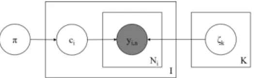
Figure 1: Plate diagram for multinomial model.

The hyperparameters are left out.

accuracy in both gold-standard dependent and independent settings.

• We use fully Bayesian posterior inference to quantify the uncertainty in parameter esti- mates.

• We provide guidelines for both model selec- tion and implementation.

Our findings indicate that models which in- clude annotator structure generally outperform other models, though unpooled models can over- fit. Several open-source implementations of each model type are available to users.

2 Bayesian Annotation Models

All Bayesian models of annotation that we de- scribe are generative: They provide a mechanism to generate parameters θ characterizing the pro- cess (annotator accuracies and biases, prevalence, etc.) from the prior p(θ), then generate the ob- served labels y from the parameters according to the sampling distribution p(y|θ). Bayesian infer- ence allows us to condition on some observed data y to draw inferences about the parameters θ; this is done through the posterior, p(θ|y).

The uncertainty in such inferences may then be used in applications such as jointly training clas- sifiers (Smyth et al., 1995; Raykar et al., 2010), comparing crowdsourcing systems (Lease and Kazai, 2011), or characterizing corpus accuracy (Passonneau and Carpenter, 2014).

This section describes the six models we eval- uate. These models are drawn from the litera- ture, but some had to be generalized from binary to multiclass annotations. The generalization nat- urally comes with parameterization changes, al- though these do not alter the fundamentals of the models. (One aspect tied to the model parameter- ization is the choice of priors. The guideline we followed was to avoid injecting any class prefer- ences a priori and let the data uncover this infor- mation; see more in §3.)

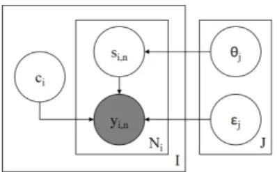
Figure 2: Plate diagram of the Dawid and Skene model.

2.1 A Pooled Model

Multinomial (M

) The simplest Bayesian model of annotation is the binomial model pro- posed in Albert and Dodd (2004) and discussed in Carpenter (2008). This model pools all annota- tors (i.e., assumes they have the same ability; see Figure 1).

The generative process is:

• For every class k ∈ {1, 2, ..., K}:

– Draw class-level abilities ζ

∼ Dirichlet(1

)

• Draw class prevalence π ∼ Dirichlet(1

)

• For every item i ∈ {1, 2, ..., I }:

– Draw true class c

∼ Categorical(π) – For every position n ∈ {1, 2, ..., N

}:

∗ Draw annotation

y

∼ Categorical(ζ

)

2.2 Unpooled Models

Dawid and Skene (D&S) The model proposed by Dawid and Skene (1979) is, to our knowledge, the first model-based approach to annotation proposed in the literature.

It has found wide application (e.g., Kim and Ghahramani, 2012; Simpson et al., 2013; Passonneau and Carpenter, 2014). It is an unpooled model, namely, each annotator has their own response parameters (see Figure 2), which are given fixed priors. Its generative process is:

• For every annotator j ∈ {1, 2, ..., J }:

– For every class k ∈ {1, 2, ..., K} :

∗ Draw class annotator abilities β

∼ Dirichlet(1

)

1Carpenter(2008) parameterizes ability in terms of specificity and sensitivity. For multiclass annotations, we generalize to a full response matrix (Passonneau and Carpenter,2014).

2Notation:1^Kis aK-dimensional vector of 1 values.

3Dawid and Skene fit maximum likelihood estimates us- ing expectation maximization (EM), but the model is easily extended to include fixed prior information for regularization, or hierarchical priors for fitting the prior jointly with the abil- ity parameters and automatically performing partial pooling.

Figure 3: Plate diagram for the MACE model.

• Draw class prevalence π ∼ Dirichlet(1

)

• For every item i ∈ {1, 2, ..., I}:

– Draw true class c

∼ Categorical(π) – For every position n ∈ {1, 2, ..., N

}:

∗ Draw annotation

y

∼ Categorical(β

)

Multi-Annotator Competence Estimation (MACE) This model, introduced by Hovy et al. (2013), takes into account the credibility of the annotators and their spamming preference and strategy

(see Figure 3). This is another example of an unpooled model, and possibly the model most widely applied to linguistic data (e.g., Plank et al., 2014a;

Sabou et al., 2014; Habernal and Gurevych, 2016, inter alia). Its generative process is:

• For every annotator j ∈ {1, 2, ..., J }:

– Draw spamming behavior

∼ Dirichlet(10

)

– Draw credibility θ

∼ Beta(0.5, 0.5)

• For every item i ∈ {1, 2, ..., I} : – Draw true class c

∼ U nif orm – For every position n ∈ {1, 2, ..., N

}:

∗ Draw a spamming indicator s

∼ Bernoulli(1 − θ

)

∗ If s

= 0 then:

· y

= c

∗ Else:

· y

∼ Categorical(

)

2.3 Partially Pooled Models

Hierarchical Dawid and Skene (H

D&S) In this model, the fixed priors of Dawid and Skene are replaced with hierarchical priors representing

4Notation: jj[i,n] gives the index of the annotator who produced then-th annotation on itemi.

5That is, propensity to produce labels with malicious intent.

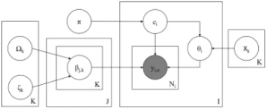
Figure 4: Plate diagram for the hierarchical Dawid and Skene model.

the overall population of annotators (see Figure 4).

This structure provides partial pooling, using in- formation about the population to improve esti- mates of individuals by regularizing toward the population mean. This is particularly helpful with low count data as found in many crowdsourcing tasks (Gelman et al., 2013). The full generative process is as follows:

• For every class k ∈ {1, 2, ..., K}:

– Draw class ability means

ζ

∼ Normal(0, 1), ∀k

∈ {1, ..., K}

– Draw class s.d.’s

Ω

∼ HalfNormal(0, 1), ∀k

• For every annotator j ∈ {1, 2, ..., J }:

– For every class k ∈ {1, 2, ..., K}:

∗ Draw class annotator abilities β

∼ Normal(ζ

, Ω

), ∀k

• Draw class prevalence π ∼ Dirichlet(1

)

• For every item i ∈ {1, 2, ..., I }:

– Draw true class c

∼ Categorical(π) – For every position n ∈ {1, 2, ..., N

}:

∗ Draw annotation y

∼

Categorical(softmax(β

))

Item Difficulty (I

D

) We also test an exten- sion of the “Beta-Binomial by Item” model from Carpenter (2008), which does not assume any an- notator structure; instead, the annotations of an item are made to depend on its intrinsic difficulty.

The model further assumes that item difficulties are instances of class-level hierarchical difficulties (see Figure 5). This is another example of a

6A two-class version of this model can be found in Carpenter(2008) under the name “Beta-Binomial by Anno- tator.”

7The argument of the softmax is aK-dimensional vector of annotator abilities given the true class, i.e.,βjj[i,n],c_i = (βjj[i,n],c_i,1, ..., βjj[i,n],c_i,K).

Figure 5: Plate diagram for the item difficulty model.

partially pooled model. Its generative process is presented here:

• For every class k ∈ {1, 2, ..., K}:

– Draw class difficulty means:

η

∼ Normal(0, 1), ∀k

∈ {1, ..., K}

– Draw class s.d.’s

X

∼ HalfNormal(0, 1), ∀k

• Draw class prevalence π ∼ Dirichlet(1

)

• For every item i ∈ {1, 2, ..., I} :

– Draw true class c

∼ Categorical(π) – Draw item difficulty θ

∼

Normal(η

, X

), ∀k

– For every position n ∈ {1, 2, ..., N

}:

∗ Draw annotation:

y

∼ Categorical(softmax(θ

)) Logistic Random Effects (L

R

E

) The last model is the Logistic Random Effects model (Carpenter, 2008), which assumes the annotations depend on both annotator abilities and item dif- ficulties (see Figure 6). Both annotator and item parameters are drawn from hierarchical priors for partial pooling. Its generative process is given as:

• For every class k ∈ {1, 2, ..., K}:

– Draw class ability means

ζ

∼ Normal(0, 1), ∀k

∈ {1, ..., K}

– Draw class ability s.d.’s Ω

∼ HalfNormal(0, 1), ∀k

– Draw class difficulty s.d.’s

X

∼ HalfNormal(0, 1), ∀k

• For every annotator j ∈ {1, 2, ..., J }:

– For every class k ∈ {1, 2, ..., K}:

∗ Draw class annotator abilities β

∼ Normal(ζ

, Ω

), ∀k

• Draw class prevalence π ∼ Dirichlet(1

)

Figure 6: Plate diagram for the logistic random effects model.

• For every item i ∈ {1, 2, ..., I }:

– Draw true class c

∼ Categorical(π) – Draw item difficulty:

θ

∼ Normal(0, X

), ∀k

– For every position n ∈ {1, 2, ..., N

}:

∗ Draw annotation y

∼

Categorical(softmax(β

−θ

))

3 Implementation of the Models

We implemented all models in this paper in Stan (Carpenter et al., 2017), a tool for Bayesian Inference based on Hamiltonian Monte Carlo.

Although the non-hierarchical models we present can be fit with (penalized) maximum likeli- hood (Dawid and Skene, 1979; Passonneau and Carpenter, 2014),

there are several advantages to a Bayesian approach. First and foremost, it pro- vides a mean for measuring predictive calibration for forecasting future results. For a well-specified model that matches the generative process, Bayesian inference provides optimally calibrated inferences (Bernardo and Smith, 2001); for only roughly accurate models, calibration may be mea- sured for model comparison (Gneiting et al., 2007). Calibrated inference is critical for mak- ing optimal decisions, as well as for forecast- ing (Berger, 2013). A second major benefit of Bayesian inference is its flexibility in combining submodels in a computationally tractable manner.

For example, predictors or features might be

8Hierarchical models are challenging to fit with classical methods; the standard approach, maximum marginal likeli- hood, requires marginalizing the hierarchical parameters, fit- ting those with an optimizer, then plugging the hierarchical parameter estimates in and repeating the process on the coef- ficients (Efron,2012). This marginalization requires either a custom approximation per model in terms of either quadra- ture or Markov chain Monte Carlo to compute the nested integral required for the marginal distribution that must be optimized first (Martins et al.,2013).

available to allow the simple categorical preva- lence model to be replaced with a multilogistic regression (Raykar et al., 2010), features of the annotators may be used to convert that to a re- gression model, or semi-supervised training might be carried out by adding known gold-standard la- bels (Van Pelt and Sorokin, 2012). Each model can be implemented straightforwardly and fit ex- actly (up to some degree of arithmetic precision) using Markov chain Monte Carlo methods, al- lowing a wide range of models to be evaluated.

This is largely because posteriors are much bet- ter behaved than point estimates for hierarchical models, which require custom solutions on a per- model basis for fitting with classical approaches (Rabe-Hesketh and Skrondal, 2008). Both of these benefits make Bayesian inference much simpler and more useful than classical point estimates and standard errors.

Convergence is assessed in a standard fash- ion using the approach proposed by Gelman and Rubin (1992): For each model we run four chains with diffuse initializations and verify that they converge to the same mean and variances (using the criterion R < ˆ 1.1).

Hierarchical priors, when jointly fit with the rest of the parameters, will be as strong and thus sup- port as much pooling as evidenced by the data. For fixed priors on simplexes (probability parameters that must be non-negative and sum to 1.0), we use uniform distributions (i.e., Dirichlet(1

)). For lo- cation and scale parameters, we use weakly infor- mative normal and half-normal priors that inform the scale of the results, but are not otherwise sen- sitive. As with all priors, they trade some bias for variance and stabilize inferences when there is not much data. The exception is MACE, for which we used the originally recommended priors, to con- form with the authors’ motivation.

All model implementations are available to readers online at http://dali.eecs.

qmul.ac.uk/papers/supplementary_

material.zip.

4 Evaluation

The models of annotation discussed in this paper find their application in multiple tasks: to label items, characterize the annotators, or flag espe- cially difficult items. This section lays out the met- rics used in the evaluation of each of these tasks.

Dataset I N J K J/I I/J

WSD 177 1770 34 3 10 10 10

10 10 10

17 20 20 52 77 177

RTE 800 8000 164 2 10 10 10

10 10 10

20 20 20 49 20 800

TEMP 462 4620 76 2 10 10 10

10 10 10

10 10 16 61 50 462

PD 5892 43161 294 4 1 5 7

7 9 57

1 4 13 147 51 3395

Table 1: General statistics (Iitems,N observations,J annotators, K classes) together with summary statis- tics for the number of annotators per item (J/I) and the number of items per annotator (I/J) (i.e., Min, 1st Quartile, Median, Mean, 3rd Quartile, and Max).

4.1 Datasets

We evaluate on a collection of datasets reflect- ing a variety of use-cases and conditions: binary vs. multi-class classification; small vs. large num- ber of annotators; sparse vs. abundant num- ber of items per annotator / annotators per item;

and varying degrees of annotator quality (statis- tics presented in Table 1). Three of the datasets—

WSD, RTE, and TEMP, created by Snow et al.

(2008)—are widely used in the literature on an- notation models (Carpenter, 2008; Hovy et al., 2013). In addition, we include the Phrase Detec- tives 1.0 (PD) corpus (Chamberlain et al., 2016), which differs in a number of key ways from the Snow et al. (2008) datasets: It has a much larger number of items and annotations, greater sparsity, and a much greater likelihood of spamming due to its collection via a game-with-a-purpose setting.

This dataset is also less artificial than the datasets in Snow et al. (2008), which were created with the express purpose of testing crowdsourcing. The data consist of anaphoric annotations, which we reduce to four general classes (DN/DO = discourse new/old, PR = property, and NR = non-referring).

To ensure similarity with the Snow et al. (2008) datasets, we also limit the coders to one annotation per item (discarded data were mostly redundant annotations). Furthermore, this corpus allows us to evaluate on meta-data not usually available in traditional crowdsourcing platforms, namely, in- formation about confessed spammers and good, established players.

4.2 Comparison Against a Gold Standard

The first model aspect we assess is how accu-

rately they identify the correct (“true”) label of

the items. The simplest way to do this is by com-

paring the inferred labels against a gold standard,

using standard metrics such as Precision / Re- call / F-measure, as done, for example, for the evaluation of MACE in Hovy et al. (2013). We check whether the reported differences are statis- tically significant, using bootstrapping (the shift method), a non-parametric two-sided test (Wilbur, 1994; Smucker et al., 2007). We use a signifi- cance threshold of 0.05 and further report whether the significance still holds after applying the Bonferroni correction for type 1 errors.

This type of evaluation, however, presupposes that a gold standard can be obtained. This as- sumption has been questioned by studies show- ing the extent of disagreement on annotation even among experts (Poesio and Artstein, 2005;

Passonneau and Carpenter, 2014; Plank et al., 2014b). This motivates exploring complementary evaluation methods.

4.3 Predictive Accuracy

In the statistical analysis literature, posterior predictions are a standard assessment method for Bayesian models (Gelman et al., 2013). We measure the predictive performance of each model using the log predictive density (lpd), that is, log p(˜ y|y), in a Bayesian K-fold cross-validation setting (Piironen and Vehtari, 2017; Vehtari et al., 2017).

The set-up is straightforward: we partition the data into K subsets, each subset formed by splitting the annotations of each annotator into K random folds (we choose K = 5). The splitting strategy ensures that models that cannot handle predictions for new annotators (i.e., unpooled models like D&S and MACE) are nevertheless included in the comparison. Concretely, we compute

lpd =

K

X

k=1

log p(˜ y

|y

)

=

K

X

k=1

log Z

p(˜ y

, θ|y

)dθ

≈

K

X

k=1

log 1 M

M

X

m=1

p(˜ y

|θ

) (1)

In Equation (1), y

and y ˜

represent the items from the train and test data, for iteration k of the cross validation, while θ

is one draw from the posterior.

4.4 Annotators’ Characterization

A key property of most of these models is that they provide a characterization of coder ability. In

the D&S model, for instance, each annotator is modeled with a confusion matrix; Passonneau and Carpenter (2014) showed how different types of annotators (biased, spamming, adversarial) can be identified by examining this matrix.

The same information is available in H

D&S and L

R

E

, whereas MACE characterizes coders by their level of credibility and spamming preference. We discuss these parameters with the help of the metadata provided by the PD corpus.

Some of the models (e.g., M

or I

D

) do not explicitly model annotators.

However, an estimate of annotator accuracy can be derived post-inference for all the models. Con- cretely, we define the accuracy of an annotator as the proportion of their annotations that match the inferred item-classes. This follows the cal- culation of gold-annotator accuracy (Hovy et al., 2013), computed with respect to the gold standard.

Similar to Hovy et al. (2013), we report the cor- relation between estimated and gold annotators’

accuracy.

4.5 Item Difficulty

Finally, the L

R

E

model also provides an estimate that can be used to assess item difficulty.

This parameter has an effect on the correctness of the annotators: namely, there is a subtractive relationship between the ability of an annotator and the item-difficulty parameter. The “difficulty”

name is thus appropriate, although an examination of this parameter alone does not explicitly mark an item as difficult or easy. The I

D

model does not model annotators and only uses the diffi- culty parameter, but the name is slightly mislead- ing because its probabilistic role changes in the absence of the other parameter (i.e., it now shows the most likely annotation classes for an item).

These observations motivate an independent mea- sure of item difficulty, but there is no agreement on what such a measure could be.

One approach is to relate the difficulty of an

item to the confidence a model has in assigning

it a label. This way, the difficulty of the items is

judged under the subjectivity of the models, which

in turn is influenced by their set of assumptions

and data fitness. As in Hovy et al. (2013), we mea-

sure the model’s confidence via entropy to filter

out the items the models are least confident in

(i.e., the more difficult ones) and report accuracy

trends.

5 Results

This section assesses the six models along dif- ferent dimensions. The results are compared with those obtained with a simple majority vote (M

V

) baseline. We do not compare the re- sults with non-probabilistic baselines as it has already been shown (see, e.g., Quoc Viet Hung et al., 2013) that they underperform compared with a model of annotation.

We follow the evaluation tasks and metrics dis- cussed in §4 and briefly summarized next. A core task for which models of annotation are used is to infer the correct interpretations from a crowd- sourced dataset of annotations. This evaluation is conducted first and consists of a comparison against a gold standard. One problem with this as- sessment is caused by ambiguity—previous stud- ies indicating disagreement even among experts.

Because obtaining a true gold standard is question- able, we further explore a complementary evalua- tion, assessing the predictive performance of the models, a standard evaluation approach from the literature on Bayesian models. Another core task models of annotation are used for is to character- ize the accuracy of the annotators and their error patterns. This is the third objective of this evalu- ation. Finally, we conclude this section assessing the ability of the models to correctly diagnose the items for which potentially incorrect labels have been inferred.

The PD data are too sparse to fit the models with item-level difficulties (i.e., I

D

and L

R

E

). These models are therefore not present in the evaluations conducted on the PD corpus.

5.1 Comparison Against a Gold Standard A core task models of annotation are used for is to infer the correct interpretations from crowd- annotated datasets. This section compares the inferred interpretations with a gold standard.

Tables 2, 3 and 4 present the results.

On WSD and TEMP datasets (see Table 4), characterized by a small number of items and annotators (statis- tics in Table 1), the different model complexi- ties result in no gains, all the models performing

9The results for MAJVOTE, HIERD&S, and LOGRNDEFF we report match or slightly outperform those reported by Carpenter (2008) on the RTE dataset.

Similar for MACE, across WSD, RTE, and TEMP datasets (Hovy et al.,2013).

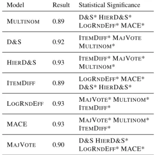
Model Result Statistical Significance MULTINOM 0.89 D&S* HIERD&S*

LOGRNDEFF* MACE*

D&S 0.92 ITEMDIFF* MAJVOTE

MULTINOM*

HIERD&S 0.93 ITEMDIFF* MAJVOTE* MULTINOM*

ITEMDIFF 0.89 LOGRNDEFF* MACE*

D&S* HIERD&S*

LOGRNDEFF 0.93 MAJVOTE* MULTINOM* ITEMDIFF*

MACE 0.93 MAJVOTE* MULTINOM* ITEMDIFF*

MAJVOTE 0.90 D&S HIERD&S*

LOGRNDEFF* MACE*

Table 2: RTE dataset results against the gold standard.

Both micro (accuracy) and macro (P, R, F) scores are the same. * indicates that significance (0.05 threshold) holds after applying the Bonferroni correction.

equivalently. Statistically significant differences (0.05 threshold, plus Bonferroni correction for type 1 errors; see §4.2 for details) are, however, very much present in Tables 2 (RTE dataset) and 3 (PD dataset). Here the results are dominated by the unpooled (D&S and MACE) and partially pooled models (L

R

E

, and H

D&S, except for PD, as discussed later in §6.1), which assume some form of annotator structure. Further- more, modeling the full annotator response matrix leads in general to better results (e.g., D&S vs.

MACE on the PD dataset). Ignoring completely any annotator structure is rarely appropriate, such models failing to capture the different levels of expertise the coders have—see the poor perfor- mance of the unpooled M

model and of the partially pooled I

D

model. Similarly, the M

V

baseline implicitly assumes equal expertise among coders, leading to poor perfor- mance results.

5.2 Predictive Accuracy

Ambiguity causes disagreement even among ex-

perts, affecting the reliability of existing gold

standards. This section presents a complementary

evaluation, namely, predictive accuracy. In a simi-

lar spirit to the results obtained in the comparison

against the gold standard, modeling the ability of

the annotators was also found to be essential for

a good predictive performance (results presented

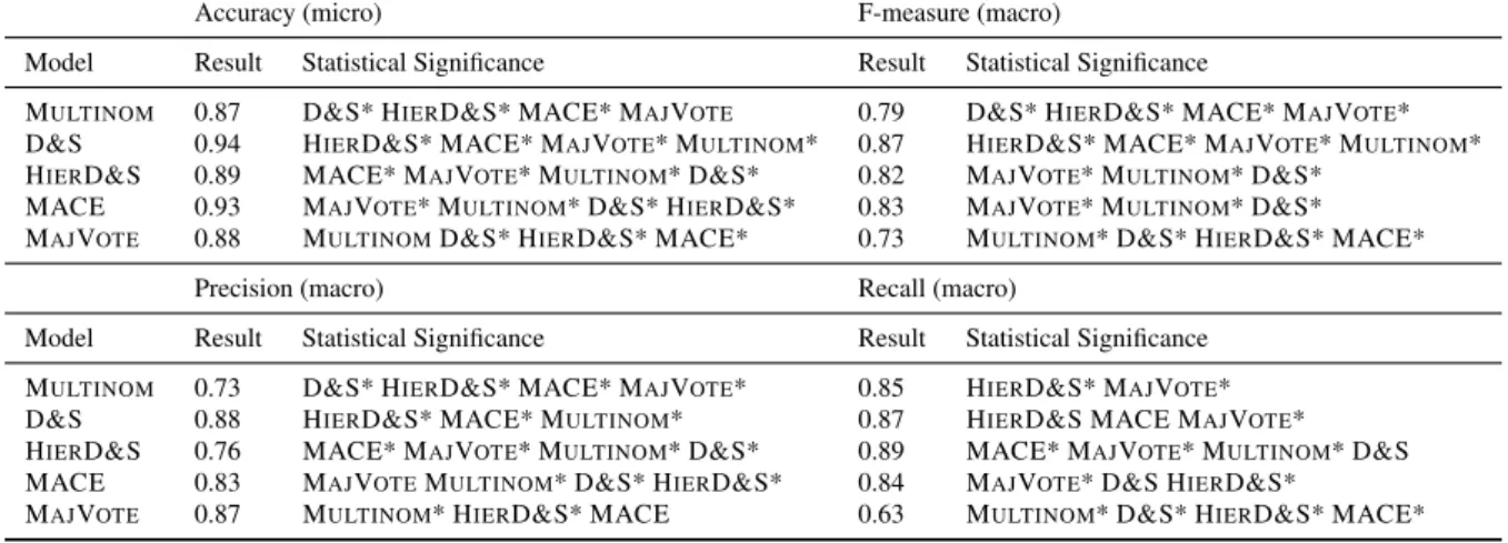
Accuracy (micro) F-measure (macro)

Model Result Statistical Significance Result Statistical Significance

MULTINOM 0.87 D&S* HIERD&S* MACE* MAJVOTE 0.79 D&S* HIERD&S* MACE* MAJVOTE* D&S 0.94 HIERD&S* MACE* MAJVOTE* MULTINOM* 0.87 HIERD&S* MACE* MAJVOTE* MULTINOM* HIERD&S 0.89 MACE* MAJVOTE* MULTINOM* D&S* 0.82 MAJVOTE* MULTINOM* D&S*

MACE 0.93 MAJVOTE* MULTINOM* D&S* HIERD&S* 0.83 MAJVOTE* MULTINOM* D&S*

MAJVOTE 0.88 MULTINOMD&S* HIERD&S* MACE* 0.73 MULTINOM* D&S* HIERD&S* MACE*

Precision (macro) Recall (macro)

Model Result Statistical Significance Result Statistical Significance MULTINOM 0.73 D&S* HIERD&S* MACE* MAJVOTE* 0.85 HIERD&S* MAJVOTE* D&S 0.88 HIERD&S* MACE* MULTINOM* 0.87 HIERD&S MACE MAJVOTE* HIERD&S 0.76 MACE* MAJVOTE* MULTINOM* D&S* 0.89 MACE* MAJVOTE* MULTINOM* D&S MACE 0.83 MAJVOTEMULTINOM* D&S* HIERD&S* 0.84 MAJVOTE* D&S HIERD&S*

MAJVOTE 0.87 MULTINOM* HIERD&S* MACE 0.63 MULTINOM* D&S* HIERD&S* MACE*

Table 3: PD dataset results against the gold standard. * indicates that significance holds after Bonferroni correction.

Dataset Model Accµ PM RM FM

WSD

ITEMDIFF

0.99 0.83 0.99 0.91 LOGRNDEFF

Others 0.99 0.89 1.00 0.94

TEMP MAJVOTE 0.94 0.93 0.94 0.94

Others 0.94 0.94 0.94 0.94

Table 4: Results against the gold (µ=Micro; M=Macro).

in Table 5). However, in this type of evaluation, the unpooled models can overfit, affecting their performance (e.g., a model of higher complex- ity like D&S, on a small dataset like WSD). The partially pooled models avoid overfitting through the hierarchical structure obtaining the best pre- dictive accuracy. Ignoring the annotator structure (I

D

and M

) leads to poor per- formance on all datasets except for WSD, where this assumption is roughly appropriate since all the annotators have a very high proficiency (above 95%).

5.3 Annotators’ Characterization

Another core task models of annotation are used for is to characterize the accuracy and bias of the annotators.

We first assess the correlation between the esti- mated and gold accuracy of the annotators. The re- sults, presented in Table 6, follow the same pattern to those obtained in §5.1: a better performance of the unpooled (D&S and MACE

) and partially pooled models (L

R

E

and H

D&S, ex- cept for PD, as discussed later in §6.1). The results

10The results of our reimplementation match the published ones (Hovy et al.,2013).

Model WSD RTE TEMP PD*

MULTINOM -0.75 -5.93 -5.84 -4.67

D&S -1.19 -4.98 -2.61 -2.99 HIERD&S -0.63 -4.71 -2.62 -3.02 ITEMDIFF -0.75 -5.97 -5.84 - LOGRNDEFF -0.59 -4.79 -2.63 -

MACE -0.70 -4.86 -2.65 -3.52

Table 5: The log predictive density results, normalized to a per-item rate (i.e.,lpd/I). Larger values indicate a better predictive performance. PD* is a subset of PD such that each annotator has a number of annotations at least as big as the number of folds.

are intuitive: A model that is accurate with respect to the gold standard should also obtain high corre- lation at annotator level.

The PD corpus also comes with a list of self- confessed spammers and one of good, established players (see Table 7 for a few details). Continuing with the correlation analysis, an inspection of the second-to-last column from Table 6 shows largely accurate results for the list of spammers. On the second category, however, the non-spammers (the last column), we see large differences between models, following the same pattern with the previ- ous correlation results. An inspection of the spam- mers’ annotations show an almost exclusive use of the DN (discourse new) class, which is highly prevalent in PD and easy for the models to infer;

the non-spammers, on the other hand, make use of all the classes, making it more difficult to capture their behavior.

11In a typical coreference corpus, over 60% of mentions are DN; thus, always choosing DN results in a good accuracy level. The one-class preference is a common spamming be- havior (Hovy et al.,2013;Passonneau and Carpenter,2014).

Model WSD RTE TEMP PD S NS

MAJVOTE 0.90 0.78 0.91 0.77 0.98 0.65

line MULTINOM 0.90 0.84 0.93 0.75 0.97 0.84

D&S 0.90 0.89 0.92 0.88 1.00 0.99

HIERD&S 0.90 0.90 0.92 0.76 1.00 0.91

ITEMDIFF 0.80 0.84 0.93 - - -

LOGRNDEFF 0.80 0.89 0.92 - - -

MACE 0.90 0.90 0.92 0.86 1.00 0.98

Table 6: Correlation between gold and estimated accu- racy of annotators. The last two columns refer to the list of known spammers and non-spammers in PD.

Type Size Gold accuracy quantiles Spammers 7 0.42 0.55 0.74

Non-spammers 19 0.59 0.89 0.94

Table 7: Statistics on player types. Reported quantiles are 2.5%, 50%, and 97.5%.

We further examine some useful parameter estimates for each player type. We chose one spammer and one non-spammer and discuss the confusion matrix inferred by D&S, together with the credibility and spamming preference given by MACE. The two annotators were chosen to be rep- resentative for their type. The selection of the mod- els was guided by their two different approaches to capturing the behavior of the annotators.

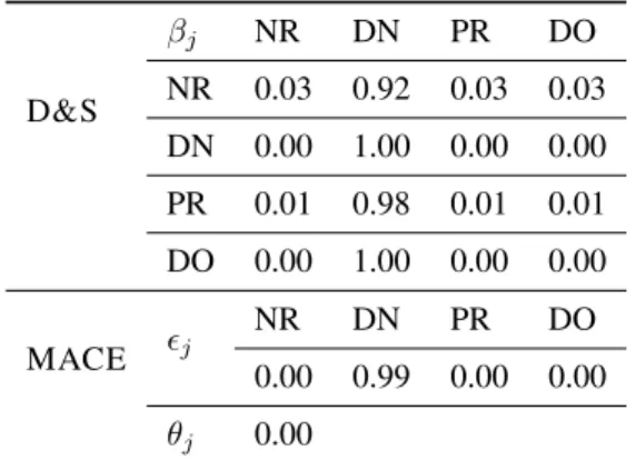
Table 8 presents the estimates for the annotator selected from the list of spammers. Again, inspec- tion of the confusion matrix shows that, irrespec- tive of the true class, the spammer almost always produces the DN label. The MACE estimates are similar, allocating 0 credibility to this annotator, and full spamming preference for the DN class.

In Table 9 we show the estimates for the anno- tator chosen from the non-spammers list. Their response matrix indicates an overall good perfor- mance (see diagonal matrix), albeit with a con- fusion of PR (property) for DN (discourse new), which is not surprising given that indefinite NPs (e.g., a policeman) are the most common type of mention in both classes. MACE allocates large credibility to this annotator and shows a similar spamming preference for the DN class.

This discussion, as well as the quantiles from Table 7, show that poor accuracy is not by it- self a good indicator of spamming. A spammer like the one discussed in this section can obtain good performance by always choosing a class with high frequency in the gold standard. At the same time, a non-spammer may fail to recognize some true classes correctly, but be very good on oth- ers. Bayesian models of annotation allow captur-

D&S

β_j NR DN PR DO NR 0.03 0.92 0.03 0.03 DN 0.00 1.00 0.00 0.00 PR 0.01 0.98 0.01 0.01 DO 0.00 1.00 0.00 0.00

MACE j

NR DN PR DO

0.00 0.99 0.00 0.00 θ_j 0.00

Table 8: Spammer analysis example. D&S provides a confusion matrix; MACE shows the spamming prefer- ence and the credibility.

D&S

βj NR DN PR DO NR 0.79 0.07 0.07 0.07 DN 0.00 0.96 0.01 0.02 PR 0.03 0.21 0.72 0.04 DO 0.00 0.06 0.00 0.94

MACE j

NR DN PR DO

0.09 0.52 0.17 0.22 θj 0.92

Table 9: A non-spammer analysis example. D&S pro- vides a confusion matrix; MACE shows the spamming preference and the credibility.

ing and exploiting these observations. For a model like D&S, such a spammer presents no harm, as their contribution towards any potential true class of the item is the same and therefore cancels out.

5.4 Filtering Using Model Confidence

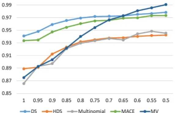
This section assesses the ability of the models to correctly diagnose the items for which potentially incorrect labels have been inferred. Concretely, we identify the items that the models are least confi- dent in (measured using the entropy of the poste- rior of the true class distribution) and present the accuracy trends as we vary the proportion of fil- tered out items.

Overall, the trends (Figures 7, 8 and 9) indicate that filtering out the items with low confidence improves the accuracy of all the models and across all datasets.

12Point also made byPassonneau and Carpenter(2014).

13The trends for MACE match the published ones. Also, we left out the analysis on the WSD dataset, as the models already obtain 99% accuracy without any filtering (see §5.1).

Figure 7: Effect of filtering on RTE: accuracy (y-axis) vs. proportion of data with lowest entropy (x-axis).

Figure 8: TEMP dataset: accuracy (y-axis) vs. propor- tion of data with lowest entropy (x-axis).

6 Discussion

We found significant differences across a number of dimensions between both the annotation models and between the models and M

V

.

6.1 Observations and Guidelines

The completely pooled model (M

) un- derperforms in almost all types of evaluation and all datasets. Its weakness derives from its core as- sumption: It is rarely appropriate in crowdsourc- ing to assume that all annotators have the same ability.

The unpooled models (D&S and MACE) as- sume each annotator has their own response pa- rameter. These models can capture the accuracy and bias of annotators, and perform well in all evaluations against the gold standard. Lower performance is obtained, however, on posterior predictions: The higher complexity of unpooled models results in overfitting, which affects their predictive performance.

The partially pooled models (I

D

, H

D&S, and L

R

E

) assume both

Figure 9: PD dataset: accuracy (y-axis) vs. proportion of data with lowest entropy (x-axis).

individual and hierarchical structure (capturing population behavior). These models achieve the best of both worlds, letting the data determine the level of pooling that is required: They asymptote to the unpooled models if there is a lot of variance among the individuals in the population, or to the fully pooled models when the variance is very low. This flexibility ensures good performance both in the evaluations against the gold standard and in terms of their predictive performance.

Across the different types of pooling, the mod- els that assume some form of annotator structure (D&S, MACE, L

R

E

, and H

D&S) came out on top in all evaluations. The unpooled models (D&S and MACE) register on par performance with the partially pooled ones (L

R

E

and H

D&S, except for the PD dataset, as discussed later in this section) in the evaluations against the gold standard, but as pre- viously mentioned, can overfit, affecting their predictive performance. Ignoring any annotator structure (the pooled M

model, the par- tially pooled I

D

model, or the M

V

baseline) leads generally to poor performance results.

The approach we took in this paper is domain- independent, that is, we did not assess and com- pare models that use features extracted from the data, even though it is known that when such fea- tures are available, they are likely to help (Raykar et al., 2010; Felt et al., 2015a; Kamar et al., 2015).

This is because a proper assessment of such mod- els would also require a careful selection of the features and how to include them into a model of annotation. A bad (i.e., misspecified in the statistical sense) domain model is going to hurt more than help as it will bias the other estimates.

Providing guidelines for this feature-based analysis

would have excessively expanded the scope of this paper. But feature-based models of annotation are extensions of the standard annotation-only mod- els; thus, this paper can serve as a foundation for the development of such models. A few exam- ples of feature-based extensions of standard mod- els of annotation are given in §7 to guide readers who may want to try them out for their specific task/domain.

The domain-independent approach we took in this paper further implies that there are no dif- ferences between applying these models to cor- pus annotation or other crowdsourcing tasks. This paper is focused on resource creation and does not propose to investigate the performance of the models in downstream tasks. However, previous work already used such models of annotation for NLP (Plank et al., 2014a; Sabou et al., 2014;

Habernal and Gurevych, 2016, image labeling (Smyth et al., 1995; Kamar et al., 2015), or med- ical (Albert and Dodd, 2004; Raykar et al., 2010) tasks.

Although H

D&S normally achieves the best performance in all evaluations on the Snow et al.

(2008) datasets, on the PD data it is outper- formed by the unpooled models (MACE and D&S). To understand this discrepancy, note that the datasets from Snow et al. (2008) were pro- duced using Amazon Mechanical Turk, by mainly highly skilled annotators; whereas the PD dataset was produced in a game-with-a-purpose setting, where most of the annotations were made by only a handful of coders of high quality, the rest be- ing produced by a large number of annotators with much lower abilities. These observations point to a single population of annotators in the former datasets, and to two groups in the latter case. The reason why the unpooled models (MACE and D&S) outperform the partially pooled H

D&S model on the PD data is that this class of mod- els assumes no population structure—hence, there is no hierarchical influence; a multi-modal hierar- chical prior in H

D&S might be better suited for the PD data. This further suggests that results depend to some extent on the dataset specifics.

This does not alter the general guidelines made in this paper.

6.2 Technical Notes

Posterior Curvature. In hierarchical models, a complicated posterior curvature increases the dif-

ficulty of the sampling process affecting con- vergence. This may happen when the data are sparse or when there are large inter-group vari- ances. One way to overcome this problem is to use a non-centered parameterization (Betancourt and Girolami 2015). This approach separates the lo- cal parameters from their parents, easing the sam- pling process. This often improves the effective sample size and, ultimately, the convergence (i.e., lower R). The non-centered parameterization of- ˆ fers an alternative but equivalent implementation of a model. We found this essential to ensure a robust implementation of the partially pooled models.

Label Switching. The label switching problem that occurs in mixture models is due to the like- lihood’s invariance under the permutation of the labels. This makes the models nonidentifiable.

Convergence cannot be directly assessed, because the chains will no longer overlap. We use a gen- eral solution to this problem from Gelman et al.

(2013): re-label the parameters, post-inference, based on a permutation that minimizes some loss function. For this survey, we used a small ran- dom sample of the gold data (e.g., five items per class) to find the permutation that maximizes model accuracy for every chain-fit. We then re- labeled the parameters of each chain according to the chain-specific permutation before combining them for convergence assessment. This ensures model identifiability and gold alignment.

7 Related Work

Bayesian models of annotation share many char- acteristics with so called item-response and ideal- point models. A popular application of these models is to analyze data associated with indi- viduals and test items. A classic example is the Rasch model (Rasch, 1993) which assumes that the probability of a person being correct on a test item is based on a subtractive relationship be- tween their ability and the difficulty of the item.

The model takes a supervised approach to jointly estimating the ability of the individuals and the difficulty of the test items based on the correct- ness of their responses. The models of annota- tion we discussed in this paper are completely unsupervised and infer, in addition to annotator ability and/or item difficulty, the correct labels.

More details on item-response models are given in

Skrondal and Rabe-Hesketh (2004) and Gelman

and Hill (2007). Item-response theory has also been recently applied to NLP applications (Lalor et al., 2016; Martınez-Plumed et al., 2016; Lalor et al., 2017).

The models considered so far take into account only the annotations. There is work, however, that further exploits the features that can accompany items. A popular example is the model introduced by Raykar et al. (2010), where the true class of an item is made to depend both on the annotations and on a logistic regression model that are jointly fit; essentially, the logistic regression replaces the simple categorical model of prevalence. Felt et al.

(2014, 2015b) introduced similar models that also modeled the predictors (features) and compared them to other approaches (Felt et al., 2015a).

Kamar et al. (2015) account for task-specific fea- ture effects on the annotations.

In §6.2, we discussed the label switching prob- lem (Stephens, 2000) that many models of an- notation suffer from. Other solutions proposed in the literature include utilizing class-informative priors, imposing ordering constraints (obvious for univariate parameters; less so in multivariate cases) (Gelman et al., 2013), or applying different post-inference relabeling techniques (Felt et al., 2014).

8 Conclusions

This study aims to promote the use of Bayesian models of annotation by the NLP community.

These models offer substantial advantages over both agreement statistics (used to judge coding standards), and over majority-voting aggregation to generate gold standards (even when used with heuristic censoring or adjudication). To provide assistance in this direction, we compare six existing models of annotation with distinct prior and likelihood structures (e.g., pooled, unpooled, and partially pooled) and a diverse set of effects (annotator ability, item difficulty, or a subtractive relationship between the two). We use various evaluation settings on four datasets, with different levels of sparsity and annotator accuracy, and report significant differences both among the models, and between models and majority voting. As importantly, we provide guidelines to both aid users in the selection of the models and to raise awareness of the technical aspects essential to their implementation. We release all models evaluated here as Stan implementations at

http://dali.eecs.qmul.ac.uk/paper/

supplementary_material.zip.

Acknowledgments

Paun, Chamberlain, and Poesio are supported by the

project, funded by

. Carpenter is partly supported by the U.S. National Science Foundation and the U.S. Office of Naval Research.

References

Paul S. Albert and Lori E. Dodd. 2004. A caution- ary note on the robustness of latent class models for estimating diagnostic error without a gold standard. Biometrics, 60(2):427–435.

Ron Artstein and Massimo Poesio. 2008. Inter- coder agreement for computational linguistics.

Computational Linguistics, 34(4):555–596.

James O. Berger. 2013. Statistical Decision The- ory and Bayesian Analysis. Springer.

José M. Bernardo and Adrian F. M. Smith. 2001.

Bayesian Theory. IOP Publishing.

Michael Betancourt and Mark Girolami. 2015.

Hamiltonian Monte Carlo for hierarchical mod- els. Current trends in Bayesian methodology with applications, 79:30.

Bob Carpenter. 2008. Multilevel Bayesian mod- els of categorical data annotation. Unpublished manuscript.

Bob Carpenter, Andrew Gelman, Matt Hoffman, Daniel Lee, Ben Goodrich, Michael Betancourt, Michael A. Brubaker, Jiqiang Guo, Peter Li, and Allen Riddell. 2017. Stan: A probabilistic programming language. Journal of Statistical Software, 76(1):1–32.

Jon Chamberlain, Massimo Poesio, and Udo Kruschwitz. 2016. Phrase Detectives corpus 1.0:

Crowdsourced anaphoric coreference. In Pro- ceedings of the International Conference on Language Resources and Evaluation (LREC 2016), Portoroz, Slovenia.

Alexander Philip Dawid and Allan M. Skene.

1979. Maximum likelihood estimation of ob-

server error-rates using the EM algorithm. Ap-

plied Statistics, 28(1):20–28.

Bradley Efron. 2012. Large-Scale Inference: Em- pirical Bayes Methods for Estimation, Testing, and Prediction, volume 1. Cambridge Univer- sity Press.

Alvan R. Feinstein and Domenic V. Cicchetti.

1990. High agreement but low kappa: I. The problems of two paradoxes. Journal of clinical epidemiology, 43(6):543–549.

Paul Felt, Kevin Black, Eric Ringger, Kevin Seppi, and Robbie Haertel. 2015a. Early gains matter:

A case for preferring generative over discrimi- native crowdsourcing models. In Proceedings of the 2015 Conference of the North American Chapter of the Association for Computational Linguistics: Human Language Technologies.

Paul Felt, Robbie Haertel, Eric K. Ringger, and Kevin D. Seppi. 2014. MOMRESP: A Bayesian model for multi-annotator document labeling. In Proceedings of the International Conference on Language Resources and Eval- uation (LREC 2014), Reykjavik.

Paul Felt, Eric K. Ringger, Jordan Boyd-Graber, and Kevin Seppi. 2015b. Making the most of crowdsourced document annotations: Confused supervised LDA. In Proceedings of the Nine- teenth Conference on Computational Natural Language Learning, pages 194–203.

Andrew Gelman, John B. Carlin, Hal S. Stern, David B. Dunson, Aki Vehtari, and Donald B.

Rubin. 2013. Bayesian Data Analysis, Third Edition. Chapman & Hall/CRC Texts in Sta- tistical Science. Taylor & Francis.

Andrew Gelman and Jennifer Hill. 2007.

Data Analysis Using Regression and Multi- level/Hierarchical Models. Analytical Methods for Social Research. Cambridge University Press.

Andrew Gelman and Donald B. Rubin. 1992. In- ference from iterative simulation using multiple sequences. Statistical science, 7:457–472.

Tilmann Gneiting, Fadoua Balabdaoui, and Adrian E. Raftery. 2007. Probabilistic fore- casts, calibration and sharpness. Journal of the Royal Statistical Society: Series B (Statistical Methodology), 69(2):243–268.

Ivan Habernal and Iryna Gurevych. 2016. What makes a convincing argument? Empirical anal- ysis and detecting attributes of convincingness in Web argumentation. In Proceedings of the 2016 Conference on Empirical Methods in Nat- ural Language Processing, pages 1214–1223.

Dirk Hovy, Taylor Berg-Kirkpatrick, Ashish Vaswani, and Eduard Hovy. 2013. Learning whom to trust with MACE. In Proceedings of the 2013 Conference of the North American Chapter of the Association for Computational Linguistics: Human Language Technologies, pages 1120–1130.

Ece Kamar, Ashish Kapoor, and Eric Horvitz.

2015. Identifying and accounting for task- dependent bias in crowdsourcing. In Third AAAI Conference on Human Computation and Crowdsourcing.

Hyun-Chul Kim and Zoubin Ghahramani. 2012.

Bayesian classifier combination. In Proceed- ings of the Fifteenth International Confer- ence on Artificial Intelligence and Statistics, pages 619–627, La Palma, Canary Islands.

John Lalor, Hao Wu, and hong yu. 2016. Build- ing an evaluation scale using item response the- ory. In Proceedings of the 2016 Conference on Empirical Methods in Natural Language Pro- cessing, pages 648–657. Association for Com- putational Linguistics.

John P. Lalor, Hao Wu, and Hong Yu. 2017.

Improving machine learning ability with fine- tuning. CoRR, abs/1702.08563. Version 1.

Matthew Lease and Gabriella Kazai. 2011.

Overview of the TREC 2011 crowdsourcing track. In Proceedings of the text retrieval con- ference (TREC).

Fernando Martınez-Plumed, Ricardo B. C.

Prudêncio, Adolfo Martınez-Usó, and José Hernández-Orallo. 2016. Making sense of item response theory in machine learning. In Proceedings of 22nd European Conference on Artificial Intelligence (ECAI), Frontiers in Artificial Intelligence and Applications, volume 285, pages 1140–1148.

Thiago G. Martins, Daniel Simpson, Finn Lindgren,

and Håvard Rue. 2013. Bayesian computing

with INLA: New features. Computational Statistics & Data Analysis, 67:68–83.

Pablo G. Moreno, Antonio Artés-Rodríguez, Yee Whye Teh, and Fernando Perez-Cruz. 2015.

Bayesian nonparametric crowdsourcing. Jour- nal of Machine Learning Research.

Rebecca J. Passonneau and Bob Carpenter. 2014.

The benefits of a model of annotation. Transac- tions of the Association for Computational Lin- guistics, 2:311–326.

Juho Piironen and Aki Vehtari. 2017. Comparison of Bayesian predictive methods for model selec- tion. Statistics and Computing, 27(3):711–735.

Barbara Plank, Dirk Hovy, Ryan McDonald, and Anders Søgaard. 2014a. Adapting taggers to Twitter with not-so-distant supervision. In Proceedings of COLING 2014, the 25th Inter- national Conference on Computational Linguis- tics: Technical Papers, pages 1783–1792.

Barbara Plank, Dirk Hovy, and Anders Sogaard.

2014b. Linguistically debatable or just plain wrong? In Proceedings of the 52nd Annual Meeting of the Association for Computational Linguistics (Volume 2: Short Papers).

Massimo Poesio and Ron Artstein. 2005. The re- liability of anaphoric annotation, reconsidered:

Taking ambiguity into account. In Proceedings of ACL Workshop on Frontiers in Corpus Anno- tation, pages 76–83.

Nguyen Quoc Viet Hung, Nguyen Thanh Tam, Lam Ngoc Tran, and Karl Aberer. 2013. An evaluation of aggregation techniques in crowd- sourcing. In Web Information Systems Engi- neering – WISE 2013, pages 1–15, Berlin, Heidelberg. Springer Berlin Heidelberg.

Sophia Rabe-Hesketh and Anders Skrondal. 2008.

Generalized linear mixed-effects models. Lon- gitudinal data analysis, pages 79–106.

Georg Rasch. 1993. Probabilistic Models for Some Intelligence and Attainment Tests. ERIC.

Vikas C. Raykar, Shipeng Yu, Linda H. Zhao, Gerardo Hermosillo Valadez, Charles Florin, Luca Bogoni, and Linda Moy. 2010. Learning from crowds. Journal of Machine Learning Re- search, 11:1297–1322.

Marta Sabou, Kalina Bontcheva, Leon Derczynski, and Arno Scharl. 2014. Corpus annotation through crowdsourcing: Towards best practice guidelines. In Proceedings of the Ninth Interna- tional Conference on Language Resources and Evaluation (LREC-2014), pages 859–866.

Aashish Sheshadri and Matthew Lease. 2013.

SQUARE: A benchmark for research on com- puting crowd consensus. In Proceedings of the 1st AAAI Conference on Human Computation (HCOMP), pages 156–164.

Edwin Simpson, Stephen Roberts, Ioannis Psorakis, and Arfon Smith. 2013. Dynamic Bayesian Combination of Multiple Imperfect Classifiers. Springer Berlin Heidelberg, Berlin, Heidelberg.

Anders Skrondal and Sophia Rabe-Hesketh. 2004.

Generalized Latent Variable Modeling: Mul- tilevel, Longitudinal, and Structural Equation Models. Chapman & Hall/CRC Interdisci- plinary Statistics. Taylor & Francis.

Mark D. Smucker, James Allan, and Ben Carterette. 2007. A comparison of statisti- cal significance tests for information retrieval evaluation. In Proceedings of the Sixteenth ACM Conference on Conference on Informa- tion and Knowledge Management, CIKM ’07, pages 623–632, New York, NY, USA. ACM.

Padhraic Smyth, Usama M. Fayyad, Michael C.

Burl, Pietro Perona, and Pierre Baldi. 1995. In- ferring ground truth from subjective labelling of Venus images. In Advances in neural informa- tion processing systems, pages 1085–1092.

Rion Snow, Brendan O’Connor, Daniel Jurafsky, and Andrew Y. Ng. 2008. Cheap and fast - but is it good? Evaluating non-expert annotations for natural language tasks. In Proceedings of the Conference on Empirical Methods in Natu- ral Language Processing, pages 254–263.

Matthew Stephens. 2000. Dealing with label switching in mixture models. Journal of the Royal Statistical Society: Series B (Statistical Methodology), 62(4):795–809.

Chris Van Pelt and Alex Sorokin. 2012. De-

signing a scalable crowdsourcing platform. In

Proceedings of the 2012 ACM SIGMOD Inter- national Conference on Management of Data, pages 765–766. ACM.

Aki Vehtari, Andrew Gelman, and Jonah Gabry.

2017. Practical Bayesian model evaluation us- ing leave-one-out cross-validation and WAIC.

Statistics and Computing, 27(5):1413–1432.

Jacob Whitehill, Ting-fan Wu, Jacob Bergsma, Javier R. Movellan, and Paul L. Ruvolo. 2009.

Whose vote should count more: Optimal in- tegration of labels from labelers of unknown expertise. In Advances in Neural Information Processing Systems 22, pages 2035–2043.

Curran Associates, Inc.

W. John Wilbur. 1994. Non-parametric signif-

icance tests of retrieval performance com-

parisons. Journal of Information Science,

20(4):270–284.