Holographic entanglement entropy: temperature and ﬂavour contributions

(1)

Holographic entanglement entropy:

temperature and flavour contributions

Nina Miekley

Munich 2015

(2)

(3)

Holographic entanglement entropy:

temperature and flavour contributions

Nina Miekley

Master’s Thesis

within the Elite Master Course Theoretical and Mathematical Physics

of Ludwig–Maximilians–Universit¨ at M¨ unchen

handed in by Nina Miekley

of Oldenburg in Holstein

(4)

Second supervisor: Dr. Michael Haack

Submission date: 18th December 2015

(5)

Abstract

This thesis investigates entanglement in strongly coupledN = 4 supersymmetric Yang- Mills theory by applying the AdS/CFT correspondence to calculate the entanglement entropy holographically. I have derived an analytic expression for the entanglement entropy at finite temperature, which agrees with known numerical results. My result has a temperature-dependent area law, which indicates a thermally induced effective mass for the adjoint degrees of freedom. This phenomenon is known as Debye screening.

Furthermore, I have considered the leading order correction to the entanglement entropy caused by coupling the theory to massive flavour degrees of freedom. My results show a mass-dependent contribution to the area law, which indicates a modification of the Debye screening. Furthermore, my findings reproduce the known results for the thermal entropy, as well as the results for the thermal potentials deduced from it.

These display the ‘meson melting’ transition between stable and unstable mesons.

(6)

(7)

Chapter 1 Introduction

In this thesis, I examine the entanglement entropy in strongly coupled N = 4 supersymmetric Yang-Mills theory (SYM theory). In quantum field theory, this measure for the quantum entanglement is difficult to calculate for higher-dimensional theories.

This is true in particular at strong coupling, where perturbative calculations are no longer possible. A promising approach to this problem is to consider a dual theory, which describes the same physics albeit looking completely different. Various dualities, where two different theories are only different formulations of the same dynamics, emerge from physics and especially from string theory. One example is the AdS/CFT correspondence, which maps N = 4 SYM theory to a five-dimensional theory containing gravity. Although gauge theory and gravity are completely different theories, the connection between them was already anticipated before the discovery of the AdS/CFT correspondence. Let us begin by looking at these arguments.

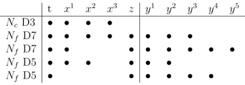
First clues

∼N² ∼N⁰

Figure 1.1: Vacuum amplitudes and corresponding string theory diagrams Picture taken from [2], scaling added

There were already clues about a link between gauge theory and string theory or gravity in the 70’s and 90’s. In 1974, ’t Hooft examined strongly coupled gauge theories with gauge groupSU(N) [1]. Since it is not possible to make an expansion in the coupling constantg_{Y M}, he treatedN as a free parameter and expanded the theory for largeN, while keeping the effective coupling constant g_{Y M}² ·N fixed. Interestingly, Feynman diagrams with scaling 1/N^2−2g can be mapped to string theory diagrams with g handles (c.f. Figure 1.1). The expansion in 1/N is therefore equivalent to an

(10)

perturbative expansion of string theory with string coupling g_s ∼ 1/N. However, the precise form of the dual string theory is unknown and is difficult to construct for higher dimensions.

The second clue was the Bekenstein entropy bound [3] and the thereby motivated holographic principle [4–6]. The Bekenstein bound states that the entropy in a volume cannot exceedA/4G_N, whereAis the boundary area andG_N is the Newton’s constant.

The holographic principle states that for a theory of quantum gravity, the degrees of freedom in a volume can be described by a theory living on the boundary, in which the degrees of freedom scale with the area. Therefore, quantum gravity in D dimensions can be described by some theory without gravity in D−1 dimensions.

AdS/CFT correspondence

In the 1960s, string theory¹ was developed to describe strong interactions. Although it was possible to describe confinement, it was not possible to describe the high energy behaviour of hadron physics and this approach was abandoned. However, string theory is a promising candidate for a unified theory describing weak force, strong force, electromagnetic force and gravity. The fundamental objects of string theory are open and closed strings. All particles are excitations of this fundamental objects. The theory automatically contains gauge symmetry as well as gravity, because gravitons are excitations of closed strings and gauge fields are excitations of open strings. However, consistency of string theory requires 10 spacetime dimensions, making it a non-trivial problem to obtain a four-dimensional theory.

In the 1970s, quantum chromodynamics (QCD) was developed to describe the strong interaction. It is SU(3) gauge theory, which is asymptotically free (i.e. has small coupling) at high energies and confined (i.e. has large coupling and only un- charged bound states exist) at low energies. As a consequence, it is not possible to perform perturbative calculations at low energy and complex numerical calculations are necessary.

In 1997, Maldacena proposed the AdS/CFT correspondence², which is motivated by dualities between different perspectives in string theory. The correspondence maps higher dimensional theories in a weakly curved spacetime to strongly coupled, large Nc conformal field theories (CFTs) with gauge group SU(Nc). The spacetime on the gravity side is Anti-de Sitter (AdS) times a compact space. Symmetry considerations place the field theory on the boundary of the AdS space, making the AdS/CFT duality a concrete realisation of the holographic principle. The additional radial coordinate in AdS is identified with the energy scale in the field theory, where the boundary corresponds to high energy and the deep bulk to low energy. Both sides of the correspondence describe the same dynamics, the same symmetries and there is a one-to-one map between operators and fields [12, 13]. The power of the correspondence is that it

1An extensive explanation of string theory is e.g. given in [7], short introductions can be found in [2, 8, 9].

2The original proposal was made in [10], reviews can be found in [2, 8, 9, 11].

(11)

3

QCD N = 4 SYM

runs to weak coupling T >>T_c remains strongly-coupled

Confinement SUSY

No confinement

T = 0 strongly-coupled plasma

(with massive fundamental matters) deconfinement, Debye screening

strongly-coupled plasma (with massive adjoint matters) deconfinement, Debye screening T >T_c

Conformal symmetry Figure 1.2: Comparison between QCD and N = 4 SYM theory

Picture taken from [2] and modified

maps physics in weakly curved gravity (i.e. a regime where we can work in appropriate approximations) to physics in a strongly coupled field theory, which is not accessible by perturbation theory.

One particularly interesting example is the duality between a field theory in four dimensions and a theory containing gravity in five dimensions. The field theory is N = 4 SU(N) supersymmetric Yang-Mills theory (or short N = 4 SYM theory), which is dual to a theory in AdS₅ ×S⁵. This duality already passed a number of non-trivial tests (e.g. the calculation of the correct three point functions and of the conformal anomaly).

Even if a dual description for QCD is not known, the AdS/CFT correspondence can provide insights into the strong coupling behaviour. The hope is that by studying supersymmetric theories, we obtain an intuition for the behaviour of strongly coupled theories and that some observables have an universal behaviour. This universal behaviour was already observed for the ratio between shear viscosity η and entropy s.

The AdS/CFT correspondence yields the famous result η/s = 1/4π [14] for a large class of strongly coupled theories, which is a small value and of the same order of mag- nitude as experimental results for QCD at high temperature. Furthermore, QCD may be similar to supersymmetric gauge theories in a specific temperature range. Above the deconfinement temperatureT_c, the theory is still strongly coupled and shares properties (e.g. Debye screening) with N = 4 SYM theory, as can be seen in Figure 1.2.

Debye screening is the phenomenon that a massless theory develops a finite correlation length due to a thermally induced mass.

(12)

B C

(a) Field theory side

B

C

(b) Gravity side

Figure 1.3: Region B on both sides

Entanglement entropy

Besides understanding local quantities like correlation functions, the AdS/CFT correspondence can also be used to study non-local properties like the entanglement entropy³. This entropy is a measure for how entangled or strongly correlated a spatial region B is with its complement C. For a global state ρ, it is defined as the von Neumann entropy of the reduced density matrix

ρ_B =Tr_Cρ,

SEE =−TrBρBlnρB.

The entanglement entropy is the missing information for an observer, who has only access to the region B but not to its complement. The physical importance of the entanglement entropy is that it is a measure for the effective degrees of freedom and can be used as an order parameter for quantum phase transitions. It is not always possible to describe such phase transitions by classical order parameter.

Although the equation for the field theory side looks simple, it involves complicated quantum calculations. There are results for two-dimensional conformal field theories, but not many for higher-dimensional theories. This makes it particularly interesting to consider a dual description. Inspired by the holographic principle and the entropy bound, Ryu and Takayanagi conjectured that the smearing out of the complement corresponds to hiding part of the bulk from the observer. The hidden information is bounded by the Bekenstein entropy bound. By minimizing the surface area of the hidden bulk volume, a bound for the corresponding entropy is found.⁴ The entanglement entropy of a region is therefore bounded byA/4G_N, whereAis the area of the minimal surface, as shown in Figure1.3. Calculations in two dimensions showed that this bound is saturated, suggesting that this is also the case in higher dimensions. Therefore, a

3For information about entanglement on the field theory side see [15–17], for the holographic dual see [18, 19] or the reviews [20, 21].

4This minimizing is performed on a constant time slice. This only works for static spacetimes, where a timelike killing field defines a unique foliation. A covariant holographic entropy was proposed in [22].

(13)

5

complicated quantum calculation reduces to a geometrical calculation. This gives a geometrical meaning to the entanglement entropy in the field theory.

Black holes

One important generalization of the AdS/CFT correspondence is the generalization to non-vanishing temperature by placing a black hole in the AdS space [23]. This connects the AdS/CFT duality to open questions in black hole physics. Black holes have laws analogous to the laws of thermodynamics. In particular, it has a temperature, whose black body radiation manifests itself as Hawking radiation [24,25], and an entropy [26].

The entropy of a black hole is the Bekenstein entropy S_BH = A

4G_N,

where A is the horizon area. For a statistical system, the entropy scales in general with the volume, hence the black hole entropy behaves like the entropy of a statistical system living in one spacetime dimension less. Furthermore, the exact origin of this entropy is an open question. In statistical mechanics, the entropy is a measure for possible microscopic states described by the same macroscopic variables. For black holes, counting the microscopic states would require a complete understanding of quantum gravity, which is not yet solved. However, semi-classical calculations of the entropy by using the saddle point approximation of the Euclidean path integral confirm the Bekenstein entropy. The AdS/CFT correspondence offers a new perspective of this entropy: the black hole entropy in AdS can be interpreted as the statistical entropy of a gauge theory living on the boundary of this space. Furthermore, since the field theory side of the correspondence is unitary, the gravity side also suspected to be unitary⁵. However, it is still an open question how unitarity is restored.

Flavour in AdS/CFT

Maldacena’s original proposal only describes adjoint degrees of freedom on the field theory side. However, it is well known that QCD also contains flavours, which are fundamental degrees of freedom. Introducing N_f flavour on the field theory side is dual to placing a stack of N_f hyperplanes in the gravity side [9, 28]. Open strings beginning at the hyperplane and falling into the bulk are transforming in the fundamental representation ofSU(N_c) and yield the fundamental degrees of freedom.

In general, the hyperplanes deform the space and it is necessary to solve the equation of motion again instead of working with the AdS background. However, some behaviour of the theory can be examined in the probe approximation, which means the deformation of the background is neglected. One example for such a property is the behaviour for massive flavour. Massive flavour are introduced by embedding the

5For a discussion, see e.g. [27].

(14)

hyperplanes non-trivially in the compact space. For zero temperature, the size of the hyperplanes shrinks to zero at some radial position and the hyperplanes end. Since the radial direction corresponds to an energy scale of the field theory, this represents a mass gap in the dual description. The quark condensate can be read of from the embedding and is vanishing at zero temperature.

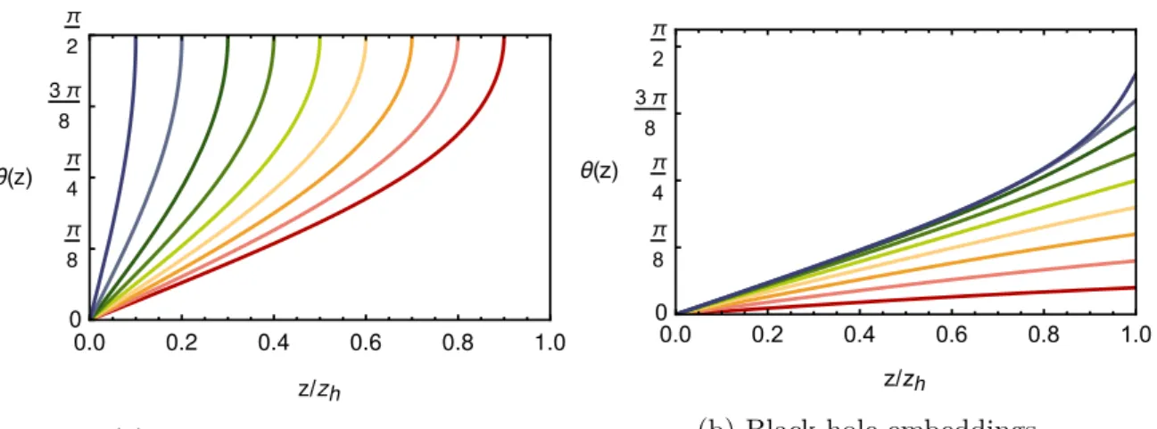
Going to non-vanishing temperature, the situation changes. The hyperplanes only fill the space outside the event horizon and there are two different kinds of embeddings:

embeddings with large mass which end before the horizon (Minkowski embeddings) and embeddings with small mass which reach the horizon (black hole embeddings).

Since the only energy scales are temperature and mass, only the ratio between them is important, making large (small) mass equivalent to low (high) temperature. It has been shown that mesons (i.e. the supersymmetric versions of a quark anti-quark bound states) are stable at low temperature, but have a finite decay time at high temperature.

The transition between this two phases is not smooth, but a first order phase transition because of a discontinuous jump between the two types of embeddings [29–32]. This phase transition is called ”meson melting”. Additionally, for non-vanishing mass and non-vanishing temperature, there is a quark condensate.⁶

However, other properties cannot be examined in this approximation, e.g. the entanglement entropy. Therefore, it is necessary to leave the probe approximation and treat the flavour as small perturbation of the background. This can be solved order by order. For the entanglement entropy, a method to calculate the leading order flavour correction was worked out in [33]. Because of the extremity of the minimizing surface, it is only necessary to calculate the area change for the same surface. This was already applied to massive flavour at zero temperature [34, 35] and massless flavour at finite temperature and charge density [36].

Results

This thesis examines the entanglement in strongly coupled N = 4 SYM theory by applying Maldacena’s AdS/CFT correspondence and Ryu’s and Takayanagi’s proposal for the holographic entanglement entropy. My results are split in two parts.

The first part analyses the entanglement entropy of the adjoint degrees of freedom in N = 4 SYM theory at finite temperature. In [18, 19], the holographic entanglement entropy for a two-dimensional conformal field theory dual to AdS₃ was calculated, while limiting the discussion of higher-dimensional cases to general arguments about the qualitative behaviour. Up to now, there are only numerical results for the holographic entanglement entropy at finite temperature in higher-dimensions (see [37]). I have obtained an analytical expressions for this entanglement entropy for a straight belt (c.f. Figure 1.3). The entanglement entropy and the width of the straight belt are expressed in terms of the turning point of the minimal surface. My results agree with the known fact that in the large-volume limit, the entanglement entropy agrees

6Chiral symmetry breaking, i.e. a quark condensate at vanishing mass, is prohibited by supersymmetry.

(15)

7

with the thermal entropy. After subtracting the thermal contribution, the ‘corrected’

entanglement entropy is lower than the zero temperature result and follows an area law in the large-volume limit, which is due to the Debye screening of the plasma.

Furthermore, I have analysed the effective degrees of freedom by a proposal for a generalized entropic c-function in [20]. The effective degrees of freedom agree with the zero temperature theory in the UV, decrease along the RG flow and vanish at the IR fixed point. This agrees with the physical interpretation that the adjoint degrees of freedom have a thermally induced mass and are integrated out in the low energy theory.

Furthermore, I calculate the leading order flavour correction to the entanglement entropy for massive flavour, following [33] and generalizing the calculations performed in [34–36]. For the backreaction of the metric, the initial conditions are chosen such that the contribution from the thermal entropy separates. The thermal entropy obtained in this thesis is used to determine the free energy and average energy, reproducing the results in [38] and showing the ‘meson melting’ phase transition. Furthermore, I examine the correction of the ‘corrected’ entanglement entropy (i.e. the entanglement entropy without thermal contribution) and compare the results with the zero temperature results. For vanishing mass, the flavour correction to the entanglement entropy is proportional to the entanglement entropy of the adjoint degrees of freedom, which was already observed for vanishing temperature. This implies that the entanglement entropy in a theory with flavour is equivalent to the entanglement entropy in a theory with increased number of adjoint degrees of freedom. For finite mass, the entanglement for a small volume is equivalent to the zero temperature result. In the large-volume limit, the entanglement approaches a constant, which is in general different from the constant of the zero temperature result. This asymptotic constant agrees with the zero temperature result for heavy flavours. Moreover, it is larger than the zero temperature result near the phase transition and lower for high temperatures. This indicates that there is a range where the effective flavour mass is lower than the effective mass of the adjoint degrees of freedom, which decreases the effects of the Debye screening. For high temperature, i.e. in the phase where mesons are melted, the temperature may induce a mass increase for the flavour degrees of freedom, which would enhance the effects of the Debye screening.

Outline

This thesis is structured as follows. The first chapter is a review of the basics of AdS/CFT. At the beginning, this chapter focuses on both sides of the duality, i.e. N = 4 SYM theory at the field theory side with additional focus on thermodynamics and the entanglement entropy as well as AdS spacetimes at the gravity side. An additionally important point in understanding the AdS/CFT correspondence and specifically its origin is string theory. Therefore, we review the key ideas with special emphasis on supergravity and D-branes. Subsequently, we state the precise form of the Maldacena’s AdS/CFT correspondence and look at the mapping between gravity theory and field

(16)

theory. A main emphasis is on adding flavour degrees of freedom and the holographic dual of the entanglement entropy.

As explained above, the results of this thesis are split into two parts. The analysis of the entanglement entropy in N = 4 SYM theory is presented in the second chapter.

The leading order flavour correction to the entanglement entropy is calculated in chapter 3. In chapter 4, I summarize my results and give an outlook on open questions. The appendix of this thesis contains a summary of conventions used (in particular of the different ranges of indices) and an overview of the AdS/CFT dictionary, which maps quantities from the gravity side to quantities of the field theory side. Furthermore, this part contains a short review of hypergeometric functions and some technical analytical calculations. Lastly, I summarize my numerical calculations.

(17)

Chapter 2 Preliminaries: AdS/CFT

In this chapter, the knowledge important for understanding my calculations is re- viewed. The starting point are the two theories the AdS/CFT correspondence relates:

conformal field theory (CFT) and gravity in Anti-de Sitter space (AdS). After briefly reviewing the basics of string theory, the origin and the exact form of the duality are summarized. Since the original duality only contains adjoint degrees of freedom, we place special emphasis on the necessary modifications to obtain flavour degrees of freedom. Furthermore, the entanglement entropy as measure for entanglement is introduced.

During preparation of this thesis, some up-to-date books about the AdS/CFT correspondence appeared, which are [2,8,39]. More information about string theory can be found in [7]. The following sections will follow these books as well as further references, as mentioned in the text.

2.1 Field theory

2.1.1 N = 4 SYM theory

N = 4 SU(N) supersymmetric Yang-Mills theory (or short N = 4 SYM theory) is a conformal field theory with R-symmetry group SU(4)_R. In the large N limit, it is exactly solveable and can be used as a simple toy model for interacting field theories in four dimensions. Let us shortly examine the different kind of symmetries in this theory.

Conformal symmetry

The conformal symmetry is a special case of Weyl symmetry. A Weyl transformation rescales the metric by multiplying a positive function

g_µν(x)→e^2σ(x)g_µν(x). (2.1)

This transformation preserves angles and causality. Conformal transformations are the restriction of Weyl transformations to flat spacetime (i.e. g_µν =η_µν). An infinitesimal

(18)

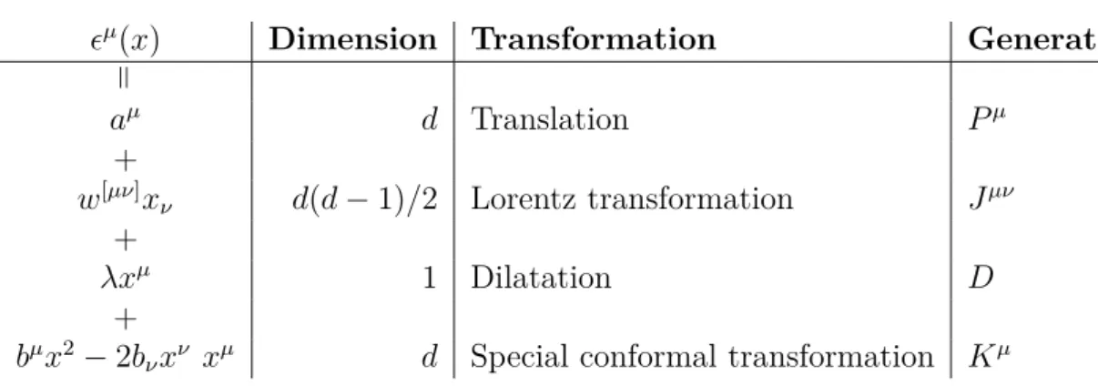
Table 2.1: Conformal transformations

^µ(x) Dimension Transformation Generator

=

a^µ d Translation P^µ

+

w^[µν]x_ν d(d−1)/2 Lorentz transformation J^µν +

λx^µ 1 Dilatation D

+

b^µx²−2b_νx^ν x^µ d Special conformal transformation K^µ conformal transformation can be achieved by the coordinate transformation

x^µ →x^µ+^µ(x), (2.2)

where satisfies the conformal Killing equation

∂_µ_ν +∂_ν_µ= 2σ(x)η_µν. (2.3) For spacetime dimension d > 2,¹ the conformal group extends the Poincar´e group with dilatations and special conformal transformations, as shown in Table 2.1. This transformation rescales the metric by multiplying exp(2σ(x)), whereσisσ =λ−2b^µx_µ. The conformal symmetry group is equivalent to SO(d,2).²

A theory which is invariant under dilatations is called scale invariant and contains only dimensionless parameters. Physically, such a theory is independent of the energy scale of interest. An infinitesimal dilatation causes δ_λg_µν = 2λδg_µν. In a classical scale invariant theory, the variation of the action vanishes, which leads to a traceless stress energy tensor.

δλS=− λ√

−g

2 T^µνgµν = 0 (2.4)

When considering a quantum theory, the expectation value of the trace can be non- vanishing due to the conformal anomaly, also called Weyl anomaly. For d = 4, the expectation value of the trace is

hT^µ_µi= c

16π²C^µνσρC_µνσρ− a

16π²E, (2.5a)

where E is the Euler topological density and C is the Weyl tensor.³

1d= 2 is special, because the conformal killing equation reduces to the Cauchy-Riemann differential equation and⁰+i¹ is an analytic (i.e. holomorphic) function ofx⁰+x¹. The symmetry group in d= 2 is infinite dimensional.

2This is the case in Minkowski signature. In Euclidean signature, it is equivalent toSO(d+ 1,1).

3The Euler topological density and the Weyl tensor are

E=R^µνσρRµνσρ−4R^µνRµν+R², Cµνσρ =Rµνσρ− 2

d−2(g_µ[σR_ρ]ν−g_ν[σR_ρ]µ) + 2

(d−1)(d−2)R g_µ[σg_ρ]ν.

(19)

2.1 Field theory 11

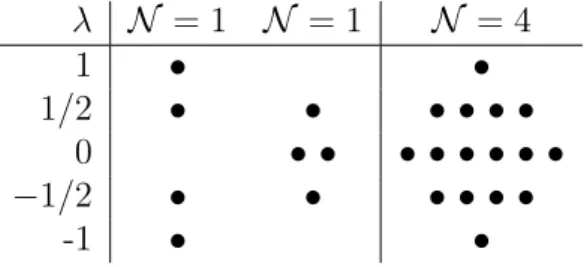
Table 2.2: Massless supersymmetric multiplets λ N = 1 N = 1 N = 4

1 • •

1/2 • • • • • • 0 • • • • • • • •

−1/2 • • • • • •

-1 • •

In general, the conformal symmetry can be broken in the renormalized theory (as happens e.g. in quantum electrodynamics).

Supersymmetry

The Coleman-Mandula theorem restricts the bosonic symmetries of a theory to Poincaré symmetry and internal symmetries. To bypass this, we have to use supersymmetry with spinor charges Qâ, a ∈ 1, . . .N. In d = 4, this charges can be written as left-handed Weyl spinor Qâ_α and right-handed Weyl spinor ¯Q_a_α_˙ = (Qâ_α)^∗, where α,α˙ ∈ {1,2} are spinor indices.⁴ When extending the Poincaré symmetry, the mass is still a Casimir operator, but the helicity is not. Qâ_α decreases the helicity by 1/2, whereas ¯Qaα˙ in- creases it by 1/2. An irreducible representation of the supersymmetry algebra has the following properties:

• same mass m for all states,

• contains states with different helicity,

• the number of fermionic and bosonic degrees of freedom agree,

• all states are in same representation of the gauge group.

The size of multiplets depends on whether they are massive or not. In a massless representation, Qâ₂ acts trivially on states, i.e. Qâ₂|physi = 0. Starting with a state of highest helicity, all 2^N states of the multiplet can be constructed by acting with Qâ₁. For CPT-invariance, we also have to add the states with negative helicity. The in the following interesting multiplets are shown in Table 2.2. The names of the multiplets depend on the highest helicity state. A gauge multiplet has λ_max = 1 and a chiral multiplet hasλ_max = 1/2.

The particle content of N = 4 SYM theory is that of the N = 4 gauge multiplet.

It has the same particle content as a N = 1 gauge multiplet and three N = 1 chiral multiplets. It is easier to obtain the unique supersymmetric theory by considering these N = 1 multiplets.

4Weyl spinors are possible in even dimensions. The dimension of a spinor is dimension-dependent, e.g. 4 ford= 4 and 16 ford= 10.

(20)

For massive multiplets, Q^a_α, α ∈ 1,2 act in a non-trivial way in general. For a special choice of algebra however, up to N/2 linear combinations (with respect to the index a= 1, . . .N) of them act trivially for both spinor indices. Therefore, the number of creation operator is reduced to 2 (N −k), yielding 2^{2(N −k)} states in the massive multiplets. This multiplets are called 1/2^k Bogomolnyi-Prasad-Sommerfield multiplets or short BPS multiplets. For this states, k of the central charges have the maximal value for a given mass m or equivalently, this states are the lightest particles for given central charges. This ensures stability of the theory.

N = 4 SU(N) supersymmetric Yang-Mills theory

The particle content of the massless N = 4 supersymmetric multiplet consists of a gauge fieldA_µ, four Weyl fermionsλ^aand six real scalarsφⁱ. All of this fields transform in the adjoint representation of SU(N). The only CP-invariant Lagrangian with the required symmetries is

L=Tr

"

− 1

2g²_{Y M}F_µνF^µν + θ

16π²F_µνF˜^µν−iλâσ¯^µD_µλ_a−D_µXⁱD^µXⁱ +gY MC_iâbλa[Xⁱ, λb] +Ciabλâ[Xⁱ, λ^b] + g_{Y M}²

2 [Xⁱ, X^j]²

#

, (2.6)

where g_{Y M} is the Yang-Mills coupling, F_µν is the field strength tensor of A^µ and C_i^ab are Clebsch-Gordan coefficients.⁵ Since the only parameter in the Lagrangian is the dimensionless coupling constant gY M, the theory is conformal on the classical level. A special feature of N = 4 SYM theory is that it is also scale invariant as a quantum theory.

Due to the conformal symmetry, the number of supercharges is doubled. The (Poincaré) supercharges Qâ,a= 1, . . .N are the superpartners ofP^µ. In a theory with conformal symmetry, we have to introduce additional (special conformal) supercharges Sâ as superpartners of K^µ. Since a spinor in four dimensions has dimension 4, this results in 32 supercharges.

2.1.2 Entanglement entropy

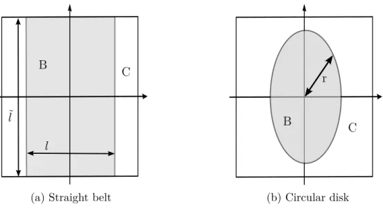
In this thesis, I calculate the entanglement entropy in N = 4 SYM theory. It is a measure for the entanglement between a spacelike submanifold B and its complement C. A common choice forB is a straight belt with widthl or a circular disk with radius r, as shown in Figure2.1. Physically, the entanglement entropy can be understood as the missing information for an observer who only has access to the region B but not to its complement. In quantum field theory, the entanglement entropy is a measure for the degrees of freedom of the theory and can be used as an order parameter for quantum phase transitions. The following review is based and the introductory papers by Calabrese [15–17], Takayanagi’s review in [19] and [40].

5Used conventions: Fµν =∂µAν−∂νAµ+i[Aµ, Aν], Dµ· =∂µ+i[Aµ,·], ¯σ^µ= −12,−σⁱ

(21)

l

˜l

B C

(a) Straight belt

r

B C

(b) Circular disk

Figure 2.1: Region B and complement C for different shapes

An observer, who does not have access to the complement C of a region B, has only access to the reduced density matrix ρ_B of the global density matrixρ

ρB = TrCρ. (2.7)

The entanglement entropyS_EE is defined as the von Neumann entropy of the reduced density matrix

SEE =−TrBρBlnρB. (2.8)

Let us have a look on how this entanglement entropy works as a measure for entanglement. We consider a pure state

ρ=|ψihψ|, (2.9)

where the Hilbert spaceH can be written as a product spaceH=H_B⊗ H_C. The state

|ψican be written in the Schmidt decomposition

|ψi=^X

i

ai|ψiiB⊗ |ψiiC, with ^X

i

|ai|² = 1, (2.10) where{|ψ_ii_B}and{|ψ_ii_C}form an orthonormal basis ofH_Band H_C respectively. The reduced density matrix is

ρ_B =Tr_Bρ,

=^X

i

|a_i|² · |ψ_ii_Bhψ_i|_B. (2.11) We see that althoughρ is pure (i.e. ^P_i|λ_i|² = 1), the reduced density matricesρ_B and ρ_C are in general not because

Tr_Bρ²_B= Tr_Cρ²_C=^X

i

|a_i|⁴. (2.12)

(22)

The entanglement entropy is

S_EE(B) = −^X

i

|a²_i|ln|a²_i|=S_EE(C) (2.13) and in general non-vanishing. It only vanishes for product states, i.e. for

|ψi=|ψi_B⊗ |ψi_C, (2.14) which means that the two subsystems are not entangled. This makes the entanglement entropy to a measure for the entanglement.

Calculating the full reduced density matrix or even only its eigenvaluesλ_iis difficult.

Due to the properties of density matrices, the eigenvalues are all positive, in the interval [0,1] and sum up to 1. Therefore, Tr_Bρⁿ_B =^P_iλⁿ_i is absolutely convergent for n ≥ 1 and can be analytically continued to Re(n) ≥ 1. This leads to the definition of the R´enyi entropies S⁽ⁿ⁾

S⁽ⁿ⁾ = 1

1−nln Tr_Bρⁿ_B. (2.15)

In the limit n →1+, this expression approaches the entanglement entropy

n→1limS⁽ⁿ⁾ = lim

n→1

−1

n−1ln (TrBρⁿ_B),

=−∂nTr_Bρⁿ_B|n=1,

=S_EE. (2.16)

Tr_Bρⁿ_B is the partition function on an n-sheeted Riemann surface, where the region B at a fixed time is removed and the boundaries are sewed together. This works well in two dimensions, but there are no exact results for higher dimensions.

This makes it difficult to prove whether a dual quantity yields the same result.

Therefore, let us take a look at some qualitative features of the entanglement entropy, which can be checked for a candidate of a dual. One well understood contribution comes from short-range correlation. At the boundary of the region, shorter and shorter correlation become important. To regulate this contribution, we introduce a UV cut-off proportional to 1/. Indspacetime dimensions, this short-range contribution yields an area law [41–43] in leading order

S_EE ∝Vol(∂B)







1

^d−2 d >2

log d= 2, (2.17)

which is proportional to the boundary of B. Together with subleading contributions, the entanglement entropy can be written as an expansion in (c.f. [44])

S_EE =cd−2(∂B)^−(d−2)+cd−1(∂B)^−(d−1)+· · ·+c₀(∂B) ln () + finite, (2.18) where only the finite part depends on the volume.

In a theory with a mass gap, the momentum of the short-range excitations is also limited from below. Therefore, we expect an additional area contribution. Further- more, the entanglement entropy has following properties

(23)

• for a pure state: S_EE(B) = S_EE(C),

• subadditivity: for a region B which is divided into B₁ and B₂

S_EE(B₁) +S_EE(B₂)≥S_EE(B), (2.19)

• strong subadditivity: for non-intersecting regions B_i

S_EE(B₁+B₂+B₃) +S_EE(B₂)≤S_EE(B₁+B₂) +S_EE(B₂+B₃). (2.20) To obtain some intuition what happens to the entanglement entropy in different situations, let us review results for two dimensions, whereB is an interval with width l. For a conformal field theory with central charge c, the entanglement entropy is

S_EE = 2c 3 log l

!

+const., (2.21)

where the last term is a non-universal constant andl is the length of the interval. The central charge c is a measure for the degrees of freedom in the theory. Since in two dimensions, the area of the boundary is the factor 2, this contains the expected area term for the UV cut-off. Using conformal mappings, this result can be generalized to non-vanishing temperatureT = 1/β, yielding

S_EE = 2c

3 log β

πsinh πl β

!!

+const.. (2.22)

Expanding this result in the large-volume limit or equivalently high-temperature limit yields

S_EE = 2c

3 log β π

!

+2cπl

3β +O(l)⁻¹+const.. (2.23) This contains the appropriate volume term for the thermal entropy. In a theory with a finite correlation lengthξ, long-range correlation decrease exponentially. For ξ l, the entanglement entropy becomes independent of the volume of the region (in two dimensions l) and only contains an area term (in two dimensions a constant).

S_EE =2c

3 log ξ

!

ξl (2.24)

Comparison to the result for non-vanishing temperature shows that, after deducing the thermal contribution, the remaining entanglement entropy contains a constant term, which is an area law for a finite correlation lengthξ = 1/(πT).

Using the entanglement entropy, it is possible to define an entropic c-function.

A c-function C is a function which depends on the renormalized coupling constants and satisfies three properties. Firstly, it is non-increasing along the renormalization group (RG) flow. Secondly, the c-function is stationary at the fixed points of the RG

(24)

flow. A stationary c-function implies that all β functions vanish and the theory is conformal. Lastly, the value of the c-function at the fixed points coincides with the central charge of the conformal theory describing the fixed point. Since the central charge is proportional to the degrees of freedom in a conformal theory, the c-function can be considered to be a measure of the degrees of freedom for a general field theory.

For two dimensions, there is a function which satisfies these conditions [45], but this is not proven for higher dimensions (see e.g. [46]). For two-dimensional theories, the c-function can be calculated by

C =ldS_EE

dl , (2.25)

where S_EE is the entanglement entropy of an interval of length l. There are many attempts to generalize this to higher dimensions. However, many are complicated to calculate. Following [20], we will use the generalization

C = l^d−1

˜l^d−2 dS_EE

dl , (2.26)

where S_EE is the entanglement entropy for a straight belt with widthl. This function is dimensionless and cut-off independent, because the cut-off dependent terms only depend on the boundary (see equation (2.18)). Furthermore, it is easy to calculate from the entanglement entropy.

2.1.3 Thermodynamics

As explained above, the entanglement entropy is a measure for the missing information for an observer in the region B. At finite temperature, there are two contributions.

The first one is the missing information about the complement C and is due to its entanglement with B. Additionally, we have to consider that the system is no longer in a pure state. It is described by thermodynamics, where a complicated many-particle system is characterized by a few macroscopic variables, which do not fix the microstate uniquely. Therefore, the entanglement entropy also contains the thermal entropy, which is associated to the missing information about the microstate. The thermal entropy dominates the entanglement entropy in the large-volume limit. This enables us to calculate the thermal entropy and thermodynamical potentials from the entanglement entropy. Thermodynamical potentials can have a physical interpretation (e.g. the average energy hEi) or give conclusions about phase transitions (e.g. the free energy F).

A system at fixed particle number, fixed volume and fixed temperatureT = 1/β is described by the canonical ensemble. The density matrix of the system is

ˆ

ρ_can = exp(−βH)ˆ

Z_can , (2.27)

(25)

where ˆH is the Hamiltonian operator and Z_can the partition function Z_can=^X

n

exp(−βE_n),

=Tr exp(−βH).ˆ (2.28)

The expectation value for operators is defined as

hOi_can= Tr (ˆρ_canO). (2.29)

One physical important expectation value is the average energy

hEi=hHiˆ can = Tr(ˆρcanH) =ˆ −∂βlnZcan. (2.30) It can be used to determine the time component of the stress energy tensor, which is the energy density. Furthermore, the diagonal spatial components are the pressureP, which is the negative density of the free energy F

F =−TlnZ_can, (2.31a)

=−P V. (2.31b)

The free energy is the thermal potential of the canonical ensemble. The von Neumann entropy is defined as

S =h−ln ˆρi_can=−Tr( ˆρ_canln ˆρ_can), (2.32a)

=−ln ˆρcan+βTrρˆcanHˆ. (2.32b) It is a measure for the missing information about the microstate. The relationship betweenF, hEi and S is

F =hEi −T S, (2.33a)

dF =−SdT −P dV +µdN, (2.33b)

where P is the pressure andµ is the chemical potential.

One interesting aspect of thermodynamics are phase transitions. They occur when the thermal potential is non-analytic at a point. This can happen when there are two competing macroscopic states and macroscopic variables determine which one is stable.

There are different kinds of phase transitions:

• first order phase transition: discontinuity of F⁰,

• second order phase transition: discontinuity of F⁰⁰ , ...

• n^th order phase transition: discontinuity of F⁽ⁿ⁾.

(26)

2.2 Gravity

Let us turn to the gravity side of the duality. The action for a spacetime is given by the Einstein Hilbert action

SEH[g_ab] = 1 16πG_N

Z

d^Dx√

−g(R−2Λ), (2.34)

where G_N is the D-dimensional Newton’s constant and Λ is the cosmological constant.

Minimizing this action yields the Einstein field equations G_ab =R_ab−1

2Rg_ab, (2.35a)

=−Λg_ab, (2.35b)

whereG_abis the Einstein tensor. In the presence of a matter contribution to the action, the Einstein field equations are sourced by the energy momentum tensor T_ab

8πG_NT_ab =G_ab+ Λg_ab, (2.36a)

Tab =− 2

√−g

δS_matter

δg^ab . (2.36b)

Taking the trace yields the scalar curvature R in terms of T and λ. This can be used to rewrite the Einstein field equations as

Rab = 8πGNT˜ab+_D−2² gabΛ, (2.37) T˜_ab =T_ab− _D−2¹ g_abT^cdg_cd. (2.38) T˜_ab is called the trace-reversed tensor.

2.2.1 AdS spacetime

For AdS/CFT, the Anti-de Sitter (or short AdS) spacetime is used on the gravity side.

It is a vacuum solution (i.e. T_ab = 0) to the Einstein field equations with negative cosmological constant Λ

R_ab−1

2Rg_ab+ Λg_ab =0. (2.39)

For any (d+ 1) dimensional solution of this equation, we immediately obtains for the scalar curvature R and the Ricci tensor R_ab as

R =d+ 1

d−12Λ, Rab = 1

d−12Λg_ab. (2.40) Hence, AdS is a spacetime with constant negative curvature. Furthermore, the AdS spacetime is a maximally symmetric spacetime (i.e. it has the maximal number of symmetries). Because of this high symmetry, the Riemann tensor is uniquely determined to be

R_abcd = R

(d+ 1)d(g_bd g_ac−g_ad g_bc). (2.41)

(27)

2.2 Gravity 19

x¹

L

qL²+ (x¹)²

Figure 2.2: AdS₂ in global coordiantes

An intuitive approach to introduce D = d + 1 dimensional AdS spacetime is by embedding it into d + 2-dimensional Minkowski spacetime R^d,2 with signature (−,+, . . . ,+,−). The AdS spacetime is the sphere with radius L.

−(X⁰)²+

n

X

i=1

(Xⁱ)²−(X^d+1)² =L². (2.42) Figure2.2 shows the embedding of AdS₂ inR³. This space is invariant under rotation in the higher dimensional spacetime, which corresponds to the group O(d,2). This group is (d+ 1)(d+ 2)/2 dimensional. This is the maximal number of independent symmetries of and+ 1 dimensional spacetime.

A common choice of coordinates are the Poincar´e patch coordinates (r, t, ~x), which are defined by

X⁰ =L²

2r 1 + r⁴

L⁴(~x²−t²+L²)

!

, (2.43a)

Xⁱ =rxⁱ

L for i∈1, . . . , d−1, (2.43b) X^d=L²

2r 1 + r⁴

L⁴(~x²−t²−L²)

!

, (2.43c)

X^d+1 =rt

L. (2.43d)

The metric in this coordinates is ds² =L²

r²dr² + r² L²

−dt²+d~x² (2.44)

and is singular atr = 0. Hence, the new coordinates are restricted tor >0 and cover only one half of the complete AdS spacetime. The other half is covered by the same

(28)

coordinates with r < 0. A similar coordinate choice is z = L²/r. The metric in this coordinates is

ds² =L² z²

dz² −dt²+d~x²= L² z²

dz²+η_νµdx^νdx^µ, (2.45) where we use Einstein sum convention and sum over µ= 1, . . . d.

2.2.2 Asymptotically AdS

We also consider less symmetric solutions of equation (2.39) in the AdS/CFT duality, which are only asymptotically AdS. This means that the metric can be written as

ds² =L² z²

dz²+ ˆgνµ(z, x)dx^νdx^µ, (2.46) which generalizes equation (2.45). This form of the metric is called Fefferman-Graham form. The metric ˆg_νµhas to be finite for z→0. An asymptotic AdS metric is singular at the boundary. However, it is still possible to define a boundary metric by using a defining function ω(z, t, ~x). If ω is smooth, positive and has a second order zero at z = 0, a boundary metric can be defined by

ds²_∂AdS = lim

z→0ω(z, t, ~x)ds²|_z=const.. (2.47) This boundary metric depends on the choice of ω. Therefore, the bulk metric only determines the boundary metric up to conformal transformations. The reason for this lies in the gauge freedom due to diffeomorphism invariance. A specific transformation of the metric is the Penrose-Brown-Henneaux transformation

z =˜z(1−2σ(˜x)), (2.48a)

x^µ=˜x^µ+a^µ(˜x,z),˜ (2.48b) with∂_za^µ =zL²g^µν∂_νσ(x) anda_µ(x,0) = 0. It keeps a metric in the Fefferman-Graham form and reduces at the boundary to an infinitesimal Weyl transformation

ˆ

gµν(0, x)→(1 + 2σ(x)) ˆgµν(0, x). (2.49) For this reason, the boundary of an asymptotically AdS spacetime is called conformal.

One example of an asymptotically AdS metric is the five dimensional AdS-Schwarzschild metric

ds²_AdS =L² z²

dz²

b(z)−b(z)dt²+d~x²

!

, (2.50a)

b(z) =1− z⁴

z_h⁴. (2.50b)

(29)

2.2 Gravity 21

Using the transformation z = ˜z/

r

1 + _4z^z^˜⁴4 h

, this can be brought to the Fefferman- Graham form with

ˆ

g_νµ(˜z, x^σ)dx^νdx^µ=−(1− _4z^˜^z⁴4 h

)² 1 + _4z^z^˜⁴4

h

dt²+ (1 +_4z^z^˜⁴4 h

)dxⁱdxⁱ. (2.51) This spacetime has an event horizon atz =z_h and contains a black hole. Expanding the metric (2.50) in Euclidean signature around the horizon yields

b(z)≈4z_h−z

z_h , (2.52a)

ds²_AdS ≈L² z_h²

dz² 4

z_h

z_h−z + 4z_h−z

z_h dτ²+d~x²

!

, (2.52b)

whereτ =it is the imaginary time. Changing the coordinates to r=L

s

1− z

z_h, (2.53a)

ϕ= 2

z_hτ (2.53b)

brings the metric to the form

ds²_AdS ≈dr²+r²dϕ²+· · · . (2.54) To avoid the conical singularity,ϕhas to be periodic with period 2π. In quantum statistical mechanics, the corresponding period of the imaginary timeβ =z_hπis identified with the inverse temperature