On-the-fly Probability Enhanced Sampling
A dissertation submitted to attain the degree of
D octor of S ciences of ETH Z urich
(Dr. sc. ETH Zurich)
presented by
M ichele I nvernizzi
MSc. in Physics Universit`a degli Studi di Milano born on 3 April 1990
citizen of Italy
accepted on the recommendation of Prof. Dr. Michele Parrinello, examiner Prof. Dr. Giovanni Bussi, co-examiner
2021
quod tales turbae motus quoque materiai significant clandestinos caecosque subesse.
multa videbis enim plagis ibi percita caecis commutare viam retroque repulsa reverti nunc huc nunc illuc in cunctas undique partis.
scilicet hic a principiis est omnibus error.
prima moventur enim per se primordia rerum, inde ea quae parvo sunt corpora conciliatu et quasi proxima sunt ad viris principiorum, ictibus illorum caecis inpulsa cientur,
ipsaque proporro paulo maiora lacessunt.
sic a principiis ascendit motus et exit paulatim nostros ad sensus, ut moveantur illa quoque, in solis quae lumine cernere quimus nec quibus id faciant plagis apparet aperte.
Lucretius, De Rerum Natura, II, 125-141
Molecular simulations have become an important scientific tool with several applications in physics, chemistry, material science and biol- ogy. Therefore, the development of more efficient and robust com- putational methods is of great importance, as any improvement in this respect can potentially have a positive impact on various open research fronts. One of the major challenges for molecular simulations is the sampling of so-called rare events, i.e. microscopic phenomena occurring on macroscopic time scales. Typical examples of rare events are phase transitions, chemical reactions, or protein folding. Here we propose a novel computational technique, called on-the-fly probability enhanced sampling (OPES) method, which can significantly improve molecular simulations of such phenomena. The OPES method can be described as an evolution of another popular enhanced sampling method, metadynamics, with respect to which it brings both concep- tual and practical improvements. It goes a long way toward making en- hanced sampling not only more efficient, but also more robust and eas- ier to use. Furthermore, OPES unifies in the same approach two tradi- tionally distinct sampling strategies, namely collective-variable-based methods and expanded-ensembles methods. We believe that this per- spective will open interesting new possibilities in the field of enhanced sampling.
Riassunto
Le simulazioni molecolari sono diventate un importante strumento
scientifico con diverse applicazioni in fisica, chimica, scienza dei mate-
riali e biologia. Pertanto, lo sviluppo di metodi di calcolo pi `u efficienti
e robusti `e di grande importanza, in quanto qualsiasi miglioramento
in questo senso pu `o potenzialmente avere un impatto positivo su va-
ri fronti di ricerca aperti. Una delle maggiori sfide per le simulazioni
molecolari `e il campionamento dei cosiddetti eventi rari, cio`e fenomeni
microscopici che si verificano su scale di tempo macroscopiche. Esem-
pi tipici di eventi rari sono le transizioni di fase, le reazioni chimiche
o il ripiegamento delle proteine. Qui proponiamo una nuova tecnica
di calcolo, chiamata metodo OPES (on-the-fly probability enhanced sam-
pling), che pu `o migliorare significativamente le simulazioni molecolari
di tali fenomeni. OPES si pu `o considerare come l’evoluzione di un al-
tro popolare metodo di campionamento potenziato, la metadinamica,
rispetto a cui apporta miglioramenti sia concettuali che pratici. OPES
ha come obiettivo di rendere il campionamento potenziato non solo pi `u
efficiente, ma anche pi `u robusto e di pi `u facile impiego. Inoltre, OPES
unifica nello stesso approccio due strategie di campionamento tradizio-
nalmente distinte, vale a dire i metodi basati su variabili collettive e
quelli basati su insiemi statistici espansi. Riteniamo che questa prospet-
tiva aprir`a nuove interessanti possibilit`a nel campo del campionamento
potenziato.
Contents v
1 Introduction 1
2 Articles 5
2.1 Coarse graining from variationally enhanced sampling applied to the Ginzburg–Landau model . . . . 5 2.2 Making the best of a bad situation: a multiscale approach to
free energy calculation . . . . 19 2.3 Rethinking metadynamics: from bias potentials to probability
distributions . . . . 43 2.4 Unified approach to enhanced sampling . . . . 65
3 Conclusion and future works 99
3.1 Conclusion . . . . 99 3.2 Future works . . . 100
Other articles 103
Bibliography 105
Acknowledgements 117
Curriculum vitae 119
Introduction
Molecular simulations are playing an ever-increasing role in modern science and are applied to fields as varied as physics, chemistry, biology, and mate- rial science. They are used for example to gain insight about the microscopic mechanisms of complex phenomena and better understand experiments or guide them, or to accelerate the discovery of new drugs and materials by pre- screening large databases of possible candidates. Since its early years, molec- ular simulation had to face two main challenges: the modelling accuracy and the sampling efficiency. Despite the tremendous progress that computer simulations have witnessed, both in hardware and algorithms, these two key challenges are still at the very center of current research and method devel- opment. During my doctoral studies, I focused on the sampling problem in molecular simulations and in this thesis I present a novel enhanced sam- pling method, called on-the-fly probability enhanced sampling (OPES), which contributes to tackling this issue.
The sampling problem has its roots in the multiscale nature of many phe-
nomena of interest such as phase transitions, protein folding or chemical
reactions, just to name a few. These phenomena, also known as rare events,
present long-lived metastable states separated by kinetic bottlenecks. The
probability of observing one of such rare transitions can be so small that,
when simulating these systems via molecular dynamics or Markov-chain
Monte Carlo, one might need an unfeasible amount of computational time
to sample all the relevant metastable states. In many practical cases most
if not all the simulation is spent in the same free energy basin, and no in-
formation about the actual phenomena is obtained. Over the years, several
different techniques have been developed to try and solve this central issue
in molecular simulations. Among them, we are interested in particular in
the so-called collective variables (CVs) based methods, the first of which was
proposed in the 70s by Torrie and Valleau [1]. Various popular enhanced
sampling methods belong to this category, such as umbrella sampling [2]
and metadynamics [3]. These methods typically add to the system a bias potential that is a function of few CVs and that artificially increases the probability of observing the rare transitions between metastable states.
These methods can efficiently solve the sampling problem only if a set of few good CVs is known for the given system. A good collective variable, or reac- tion coordinate, should encode all the slow modes of the system and express them as a smooth function of the atomic positions. As a consequence, such CVs should be able to distinguish all the relevant metastable states as well as the transition states in between them. Typically, CVs are carefully devised by trial and error, guided by human insight and expertise, but this process can be difficult and time-consuming and quickly becomes impractical for complex systems. For this reason, in recent years much effort has been de- voted to try to apply machine learning techniques to automatically find such good CVs. The interested reader can find in Ref. [4] a good (even though inevitably incomplete) review of this still very active field of research.
With my research I have taken instead a different direction and studied the way the bias potential can be built, rather than focusing on the identification of CVs. This choice was motivated by the experience gained by me and other colleagues in the research group while making use of metadynamics and the variationally enhanced sampling (VES) method [5]. Although these methods can be extremely powerful, allowing the study of elusive phenom- ena, it was clear to us practitioners that they could be further improved. A first aspect that I wanted to tackle was the slow convergence of the methods when suboptimal CVs are used, thus when some slow mode is not accel- erated by biasing. Fewer transitions and hysteresis are clear symptoms of this suboptimality, and in this scenario the choice of the parameters of the methods becomes delicate, often requiring a trial-and-error approach. The outcome of my research has been a novel enhanced sampling method, OPES, that brings not only an improvement over some of these practical aspects, but also a different perspective on enhanced sampling. The method inherits some key characteristics from metadynamics and VES, such as the on-the- fly optimization of the bias, or the concept of target probability distribution, which is pushed even further, bringing new insight into what enhanced sam- pling can be.
This thesis is made as a compilation of four articles that are connected to the development of the OPES method. The first two articles, Sec. 2.1 and 2.2, do not directly deal with OPES, but are instead based on the VES method.
They are included in the thesis because they present some of the key ideas
that later have contributed to the formulation of the OPES method, and
thus can guide the reader to better understand the underlying issues and
the tools that are at the heart of the new method. In the last two articles,
Sec. 2.3 and 2.4, the OPES method is formulated and applied to some pro-
tions and, while its core elements remain the same, the implementation can
change considerably depending on the chosen target. In the first of these
two articles, similarly to metadynamics, OPES is used to sample uniform
or well-tempered distributions in the CV space and makes use of a kernel
density estimation algorithm. On the contrary, in the last paper we explore
the exciting possibility of using the OPES formalism to perform the same
type of sampling as the popular replica-exchange method[6], thus targeting
expanded ensembles. This last article proves that the perspective introduced
with OPES has been able to bring new insights into the field of enhanced
sampling that go beyond the practical improvements that I was aiming for
at the beginning of my research. Finally, in the concluding chapter of this
thesis I discuss possible future research routes and applications of the OPES
method.
Articles
2.1 Coarse graining from variationally enhanced sam- pling applied to the Ginzburg–Landau model
This first article is not directly related to the OPES method, however, thanks to its unusual perspective on enhanced sampling, it touches on some ideas that were later crucial to develop the method. The goal of this paper is to show how the variationally enhanced sampling method can be used to efficiently optimize the parameters of a coarse-graining model, while simul- taneously improving the sampling of the underlying full-atoms system. We also explore the use of a nontrivial target distribution and we show that by using a simple functional to model the free energy (only three free parame- ters), it becomes possible to greatly increase the number of employed CVs (up to 364 in the paper). This idea of taking advantage of a specific func- tional form to express the bias, was later used for developing the expanded ensemble version of OPES, Sec. 2.4.
My contribution to this article has been implementing the algorithms, per- forming the simulations, and writing the paper jointly with Valsson and Prof. Parrinello.
Reference: M. Invernizzi, O. Valsson, and M. Parrinello. “Coarse grain- ing from variationally enhanced sampling applied to the Ginzburg-Landau model.” Proceedings of the National Academy of Sciences 114.13 (2017): 3370- 3374. URL https://www.pnas.org/content/114/13/3370
Copyright © 2017 National Academy of Sciences.
Coarse graining from variationally enhanced sampling applied to the Ginzburg–Landau model
Michele Invernizzi
1,2, Omar Valsson
3,2, and Michele Parrinello*
3,21
Department of Physics, ETH Zurich c/o Universit`a della Svizzera italiana, 6900 Lugano, Switzerland
2
Facolt`a di Informatica, Institute of Computational Science, and National Center for Computational Design and Discovery of Novel Materials (MARVEL), Universit`a della
Svizzera italiana, 6900 Lugano, Switzerland
3
Department of Chemistry and Applied Biosciences, ETH Zurich c/o Universit`a della Svizzera italiana, 6900 Lugano, Switzerland
Abstract
A powerful way to deal with a complex system is to build a coarse- grained model capable of catching its main physical features, while be- ing computationally affordable. Inevitably, such coarse-grained models introduce a set of phenomenological parameters, which are often not easily deducible from the underlying atomistic system. We present a unique approach to the calculation of these parameters, based on the recently introduced variationally enhanced sampling method. It allows us to obtain the parameters from atomistic simulations, providing thus a direct connection between the microscopic and the mesoscopic scale.
The coarse-grained model we consider is that of Ginzburg-Landau, valid around a second order critical point. In particular we use it to describe a Lennard-Jones fluid in the region close to the liquid-vapor critical point. The procedure is general and can be adapted to other coarse-grained models.
2.1.1 Introduction
Computer simulations of condensed systems based on an atomistic descrip- tion of matter are playing an ever-increasing role in many fields of science.
Yet, as the complexity of the systems studied increases, so does the aware- ness that a less detailed, but nevertheless accurate, description of the system is necessary.
This has been long since recognized, and branches of physics like elastic-
ity or hydrodynamics can be classified in modern terms as coarse-grained
(CG) models of matter. In more recent times, a field theoretical model suit-
able to describe second order phase transitions has been introduced by Lan-
dau [7], and later perfected by Ginzburg [8]. In recent decades a number
of coarse-grained models that aim at describing polymers or biomolecules
have also been proposed [9, 10]. In all these approaches some degrees of free-
dom, deemed not essential to study the phenomenon at hand, are integrated
out and the resulting reduced description contains a number of parameters
which are not easy to be determined.
Here we shall use the recently developed variationally enhanced sampling (VES) method [5] to suggest a procedure that allows the determination of such parameters, starting from the microscopic Hamiltonian. This will il- luminate a somewhat unexpected application of VES, which has been intro- duced as an enhanced sampling method. We shall show that it also provides a powerful framework for the optimization of CG models, thanks to the com- bination of its enhanced sampling capabilities and its variational flexibility.
Moreover VES takes advantage of its deep connection with relative entropy, a quantity that has been shown to play a key role in multiscale problems [11, 12].
As a first test case for our procedure we shall consider the Ginzburg-Landau (GL) model for continuous phase transitions. An advantage of using this model is that its strengths and limits are well known and that other re- searchers have already attempted to perform such a calculation [13–19]. A system which undergoes a second order phase transition is described in the GL model by the following free energy, valid in a rotationally invariant one-component real order parameter scenario:
F [ ψ ] = g Z
|∇ ψ ( ~ r )|
2d
3r + a Z
ψ
2( ~ r ) d
3r + b Z
ψ
4( ~ r ) d
3r , (2.1) where the field ψ ( ~ r ) describes the order parameter fluctuations, and g, a and b are phenomenological quantities that we shall call Landau’s parameters.
To be defined, we shall apply our method close to the liquid-vapor critical point of a Lennard-Jones fluid.
2.1.2 Variationally Enhanced Sampling
Before discussing our method, we briefly recall some of the ideas at the basis of VES. The VES method shares with metadynamics [3, 20] the idea of enhancing the sampling by adding an external bias potential, which is a function of a few coarse-grained order parameters, so-called collective vari- ables (CVs). Contrary to metadynamics and other similar methods, VES does not generate the bias potential by periodically adding on the fly small contributions, but as the result of the minimization of a convex functional.
Various extensions have been proposed, where VES has been employed in different ways [21–26].
Let’s suppose that the physical behavior of interest is well described by a set of CVs s = s ( R ) , that are function of the coordinates R of the N particles that compose the system. Then one can write the associated free energy function as F ( s ) = −( 1/β ) log R
dR δ [ s − s ( R )] e
−βU(R), where β = 1/ ( k
BT )
is the inverse temperature and U ( R ) is the interparticle potential energy.
In VES a functional that depends on an externally applied bias V ( s ) is intro- duced:
Ω [ V ] = 1 β log
R ds e
−β[F(s)+V(s)]R ds e
−βF(s)+
Z
ds p ( s ) V ( s ) , (2.2) where p ( s ) is a chosen probability distribution, that we will call target dis- tribution. The functional is convex and for the value of V ( s ) that minimizes Ω [ V ] , one has
P
V( s ) = p ( s ) , (2.3)
where
P
V( s ) = e
−β[F(s)+V(s)]
R ds e
−β[F(s)+V(s)](2.4) is the distribution of s in the ensemble biased by V ( s ) . Neglecting immate- rial constants, Eq. (2.3) can also be written as
F ( s ) = − V ( s ) − 1
β log p ( s ) . (2.5)
Thus, finding the minimizing bias potential V ( s ) is equivalent to finding the free energy F ( s ) .
We notice here that the functional Ω [ V ] has close connections to the relative entropy or Kullback-Leibler divergence D
KL[27–29], in particular βΩ [ V ] = D
KL( p k P
V) − D
KL( p k P
0) . Furthermore, at the minimum we have Ω [ V ] ≤ 0, which is a rewrite of the Gibbs-Bogoliubov inequality [30].
In order to minimize Ω [ V ] we shall express V ( s ) as a linear function of a finite set of variational parameters α = { α
i} , thus V ( s; α ) . By doing so, our functional becomes a function of α, that can be minimized using the gradient and the Hessian
∂ Ω ( α )
∂α
i= −
∂V ( s; α )
∂α
iV(α)
+
∂V ( s; α )
∂α
ip
(2.6)
∂
2Ω ( α )
∂α
i∂α
j= β
"
∂V ( s; α )
∂α
i∂V ( s; α )
∂α
jV(α)
−
∂V ( s; α )
∂α
iV(α)
∂V ( s; α )
∂α
jV(α)
#
, (2.7)
where the averages in the right hand side of the equations are calculated ei- ther in the biased ensemble h·i
V(α), or in the p ( s ) ensemble h·i
p, and second derivatives in α have been omitted due to the linearity assumption.
Since the forces in Eq. (2.6,2.7) are calculated as statistical averages, a stochas-
tic optimization method [31] is needed. We describe in detail the minimiza-
tion procedure in the Supporting Information (Sec. 2.1.9).
2.1.3 Free Energy Model
We consider a Lennard-Jones fluid of N particles confined in a periodically repeated cubic box of volume V = L
3. The order parameter of such a system is linked to the density ρ ( ~ r ) :
ψ ( ~ r ) = ρ ( ~ r ) − ρ
cρ
0, (2.8)
where ρ
0= N/V and ρ
cis the critical density. The order parameter can be expanded in a discrete Fourier series as:
ψ ( ~ r ) = ∑
~k
e
i~k·~rψ
~k, (2.9)
where ~ k =
2πL~ n, with ~ n ∈ Z
3. Ginzburg-Landau model implicitly relies on a characteristic CG length Λ. This is defined by including in the series expansion, Eq. (2.9), only those wave vectors ~ k whose modulus is less than k
M= 2π/Λ. We will refer to this as “wave vector cutoff of order n
M”, where n
Mis an integer such that | ~ k |
2≤ k
2M= n
M( 2π/L )
2for all the included ~ k.
Close to T
cthe system is dominated by long wavelength fluctuations and the presence of a cutoff should become physically irrelevant.
We shall consider as collective variables these Fourier components of the order parameter, s = { ψ
~k}
|~k|≤kM
. In terms of s the GL free energy can be rewritten as
F ( s ) = g I
G( s ) + a I
2( s ) + b I
4( s ) , (2.10) where the integrals in Eq. (2.1) are rewritten in Fourier space as:
I
G( s ) = V ∑
|~k|≤kM
k
2| ψ
~k|
2(2.11)
I
2( s ) = V ∑
|~k|≤kM
| ψ
~k|
2(2.12)
I
4( s ) = V ∑
|~q|≤2kM
∑
|~k|≤kM
ψ
~kψ
~q−~k2
(2.13)
and in the last convolution it is implied that if | ~ q − ~ k | > k
Mthen ψ
~q−~k= 0. We notice that since the order parameter is a real quantity, its Fourier transform has the property ψ
~k= ψ
∗−~k
. This symmetry property will be used
to reduce the number of independent collective variables. With a cutoff of
order n
M= 3 one has 26 CVs, but in our simulations we have dealt with up
to 364 CVs, in the n
M= 19 case (see Table 2.1).
T>T
cψ F(T,ψ)
T=T
cψ F(T,ψ)
T<T
cψ F(T,ψ)
Figure 2.1:
A simplified one-dimensional representation of the chosen quadratic target free energy
Ft= −(
1/β)
logp(
s) (green dashed line) and the expected Landau’s free energy (orange solid line).
2.1.4 Bias Potential and Target Distribution
In order to proceed, we have to choose a variational form for V ( s ) and intro- duce a suitable p ( s ) . We shall use for V ( s ) and p ( s ) expressions that, when combined as in Eq. (2.5), lead for F ( s ) to an expression with the same ana- lytical structure as the GL free energy, Eq. (2.10). Guided by this principle we take
V ( s ) = g
VI
G( s ) + a
VI
2( s ) + b
VI
4( s ) (2.14) and
p ( s ) = e
−β[gtIG(s)+atI2(s)]
R ds e
−β[gtIG(s)+atI2(s)]. (2.15) These two expressions can be employed in Ω [ V ] , which then can be min- imized relative to the variational parameters g
V, a
Vand b
V. At the min- imum the estimated F ( s ) has the desired GL structure, with parameters g = g
t− g
V, a = a
t− a
Vand b = − b
V.
Since V ( s ) in Eq. (2.14) has only a limited variational flexibility, our estimate of the free energy F ( s ) is only approximated. However, given that our V ( s ) is based on sound physical considerations, we still expect the F ( s ) obtained to be a good approximation.
Using the p ( s ) in Eq. (2.15) has some advantages. It is a product of uni- variate Gaussian distributions, so the averages over p ( s ) that are needed to minimize Ω [ V ] (see Eq. 2.6,2.7) can easily be evaluated. And, more im- portantly, it can be used to guide sampling and accelerate the optimization convergence.
In order to understand this point we shall refer to Fig. 2.1 that gives an
artist’s impression of a Landau free energy as a function of a one dimen-
sional order parameter as the system crosses the critical temperature T
c. For
T > T
cthe order parameter fluctuations are predominantly Gaussian and
the effect of the non-Gaussian quartic term is hidden in the tail of the distri-
bution, as pointed out also by other authors [15, 18]. By using a p ( s ) that is
broader than the natural Gaussian fluctuations, we can enhance the proba- bility with which the tails are sampled, thus improving the computation of the parameter b proportional to the quartic term I
4( s ) .
For T < T
cone enters into the coexistence region, where different problems arise. The symmetry is broken, and the system spontaneously separates into two slab-shaped regions of finite but different value of the order parameter.
These two phases, vapor and liquid, correspond to the two minima in the rightmost curve in Fig. 2.1. By using a p ( s ) that focuses on the transition region we can keep the system homogeneous and avoid to a certain extent some finite-size drawbacks (see Ref. [32]). However, as the temperature is lowered, the interface between the two phases sharpens up with respect to the CG length Λ. This situation cannot be described quantitatively by a GL model which takes into account only long wavelengths fluctuations of the order parameter. In our simulations there are some clear evidences that the underlying model is not any longer suited for describing the system. In fact the convergence in the optimization of Ω [ V ] slows dramatically, and the obtained parameters no more follow the expected linear behavior.
The use of a higher wave vector cutoff, and thus a smaller CG length Λ, can mitigate this issue, but only marginally. In fact there is another important feature that is not taken into account by this simple model, that is the so called field-mixing due to the lack of particle-hole symmetry [33], which in- duces an asymmetry between the two phases at low T. Nevertheless the GL model we adopted can still give us some relevant information, as shown at the end of Sec. 2.1.6.
2.1.5 Computational Setup
We choose to simulate an Argon fluid, described by the classical two body Lennard-Jones potential ϕ
LJ( r ) = 4ε [( σ/r )
12− ( σ/r )
6] truncated and shifted at R
c= 2.5σ :
Φ
LJ( r ) = (
ϕ
LJ( r ) − ϕ
LJ( R
c) r < R
c0 r ≥ R
c(2.16)
This simple system has been intensively studied [32–35] and exhibits in its phase diagram the needed second order phase transition, at the liquid-vapor critical point. All the physical quantities in this paper are expressed in terms of Lennard-Jones reduced units.
We perform canonical (NVT) molecular dynamics simulations at a fixed
average density equal to the critical one, ρ
c= 0.317 (see Ref. [34]). We are
aware that in a finite size system the critical density is not exactly ρ
c, but for
our purposes we just need to be close to that value. The temperature T is
kept constant by the velocity rescaling stochastic thermostat [36]. The time
step used is 0.002, and typically we used 10
7steps for each run.
−0.1 0 0.1
(a) (b)
−0.1 0 0.1
0.8 1.0 1.2
Landau Parameters
Temperature T/Tc (c)
0.8 1.0 1.2
(d) g
a b
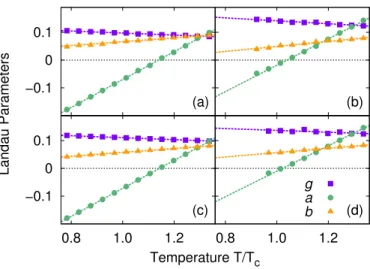
Figure 2.2:
Landau’s parameters optimized for systems with: (a)
N=
128, nM=
3thus
Λ=
4.267; (b)N=
2048, nM=
3thus
Λ=
10.75; (c) N=
2048,nM=
19thus
Λ=
4.272;(d)
N=
8192, nM=
3thus
Λ=
17.07. Data at temperatures where convergence was not clearly reachable are omitted. The linear fits are obtained using only data at
T>
0.95Tc, and error bars are smaller than the data points.
All the simulations are performed with the molecular dynamics package GROMACS 5.0.4 [37], patched with a development version of the PLUMED 2 [38] enhance sampling plugin, in which we implemented the VES method for our specific GL free energy model.
The choice of g
tand a
t, that define p ( s ) in Eq. (2.15), was based on the amplitude of the fluctuations observed in the unbiased runs, and on some trial and error simulations performed on small systems (N = 128, 256). The value thus obtained were then used as reference for the larger systems. The adopted values were between 0.05 and 0.2, and generally g
t> a
t.
2.1.6 Results
Ginzburg-Landau model expects the parameter a to have a linear tempera- ture dependence close to the critical point, thus
a ( T ) = a
c( T − T
c) , (2.17)
while the other two parameters should be constant, g ( T ) = g
cand b ( T ) =
b
c. We run multiple simulations varying both, the size of the system and
the cutoff order, and consequently also the CG length Λ . As noted at the
end of Sec. 2.1.4, depending on the system size and Λ, convergence can
become problematic at low temperatures. Nevertheless we can, somewhat
conservatively, refer only to the region T > 0.95 T
c, where convergence is
safely reached for all the systems studied here. In this region our estimates
are always in qualitative agreement with Landau’s ansatz, as can be seen e.g.
1.140 1.101 1.196 1.077 1.132 1.211
1.054 1.091 1.141 1.177
1.039 1.064 1.098 1.119 1.143
1.028 1.045 1.066
1.022 1.033
1 / 8192 1 / 2048 1 / 512 1 / 128 1 / N
5 10 15 20
n
M3 7 11 15
Λ
Figure 2.3:
The effective critical temperature
Tc∗/Tcfor different system sizes
Nand wave vector cutoff orders
nM. The dimension of the points is proportional to (
Tc∗/Tc−
1) . The background colors are related to the coarse-graining length
Λ ∝N1/3/√
nM
, according to the scale on the right.
in Fig. 2.2. The temperature dependence of the three parameters can be well fitted linearly, and all the results obtained are provided in the Supporting Information (Sec. 2.1.9). Here we only notice that the slope of g ( T ) and b ( T ) is roughly 10 times smaller than the one of a ( T ) . This non-constant behavior has been reported also in previous literature, for other Landau free energy models (see e.g. Ref. [15]).
It is possible to define an effective critical temperature T
c∗, as the temperature at which the parameter a ( T ) becomes zero. This is different from the critical temperature in the thermodynamic limit, T
c= 1.085 ± 0.005 [34], due to finite size effects. Contrary to the effective critical temperature that one could define by looking at the specific heat, T
c∗is always greater than T
c, as noted already in Ref. [13]. In Fig. 2.3 we show our estimate of T
c∗/T
cas a function of both the system size N, and the wave vector cutoff order n
M. As expected, increasing the size at fixed cutoff we have that T
c∗approaches T
c. Maybe less intuitively, when we increase the number of wave vectors, T
c∗moves away from T
c. What we observe is that T
c∗is mainly linked to the coarse-graining length Λ, in fact we find that roughly ( T
c∗− T
c) ∝ 1/Λ. In spite of the great variations in the value of T
c∗, all our data on a ( T ) can be collapsed into a single line when plotted as a function of ( T − T
c∗) /T
c, see Fig. 2.4. These are all empirical observations and do not necessarily imply rigorous scaling laws.
2.1.7 Simulations of the coarse-grained model
Having obtained a coarse-grained description, we can ask to what an ex- tent the GL model can represent the microscopic properties of the system.
To try and answer this question, we run Monte Carlo simulations, using as
−0.1 0.0 0.1 0.2
−0.2 0.0 0.2 0.4
Parameter a
Temperature (T−T*c)/Tc
5 9 13 17
Λ
Figure 2.4:
Parameter
a, the one proportional to the quadratic term in Eq. (2.10), as a functionof the rescaled temperature (
T−
Tc∗)
/Tc. The effective critical temperature
Tc∗is different for each system, as shown in Fig. 2.3. Only points with
T>
0.95Tcare plotted.
variables the Fourier components ψ
~kand as Hamiltonian the GL free energy.
We define the model at all temperatures by assuming that the parameters de- pend linearly on T. Despite the limitations of GL model (see end of section 2.1.4), we find that some of the properties of our system are well described for a wide range of temperatures.
The most remarkable one is maybe the description of the Binder cumulant [39, 40], a quantity often used to obtain a good estimate of the critical tem- perature T
c, from finite-size simulations. Using our notation, we can handily express the Binder cumulant as follows:
U ( T ) = 1 − h I
4i
3 h I
2i
2, (2.18)
where h·i is the ensemble average at temperature T, and I
2and I
4are defined in Eq. (2.12,2.13) respectively. The important property of Binder cumulant is that U ( T
c) does not depend on the system size, and thus it is possible to evaluate T
cby looking at the crossing point of the curves obtained with different N.
The behavior of U ( T ) for different system sizes is reported in Fig. 2.5, as ob-
tained with unbiased molecular dynamics and Monte Carlo coarse-grained
simulations. Remarkably the CG simulations well reproduce the U ( T ) curve,
even at T < T
c, and gives an estimate of T
Cin good agreement with the liter-
ature [34]. To calculate I
2and I
4for this figure we have used a wave vector
cutoff of order n
M= 3, but it is important to note that the inclusion of
higher order wave vectors does not change the crossing point, even though
the shape of the curves U ( T ) may change. This reflects the fact that the
critical behavior is dominated by long wavelength fluctuations.
0 0.1 0.2 0.3 0.4 0.5
0.8 0.9 1.0 1.1 1.2 1.3
Binder Cumulant U(T)
Temperature T/Tc N=128 N=512 N=2048 N=8192
Figure 2.5:
The Binder cumulant
U(
T) defined in Eq. (2.18) obtained with full molecular dynamics simulations and with Monte Carlo simulations using the optimized GL free energy as Hamiltonian. In both cases a wave vector cutoff of order
nM=
3was used, thus for the CG simulations only
26independent variables were employed for each system size. The interception of the curves gives an estimate of the critical temperature. We take as reference
Tc=
1.085[34].
Error bars are smaller than the data points, and lines are only drawn to guide the eyes.
2.1.8 Conclusions
In this paper we have shown that VES is not only a method for enhanced sampling, but it provides a formidable tool to approach coarse-graining in a systematic and rigorous way. It combines the strength of relative entropy optimization methods with the intriguing ability to orient the sampling to- wards a desired statistical distribution.
In the present application we treated the case of a second order phase tran- sition, for which the well established GL theory provided a good CG model.
In other fields of application careful consideration will have to be paid, and the structure of the CG model might not be easily determinable. However once this is done, VES provides a way to link rigorously and effectively the parameters of the coarse-graining model to the microscopic Hamiltonian.
Aknowledgements
This research was supported by the NCCR MARVEL, funded by the Swiss
National Science Foundation, and the European Union Grant No. ERC-2014-
AdG-670227/VARMET. The computational time for this work was provided
by the Swiss National Supercomputing Center (CSCS). The authors thank
Haiyang Niu for carefully reading the manuscript.
2.1.9 Supporting Information
Minimization Procedure
The minimization of the VES functional Ω [ V ] , Eq. (2.2), was carried out following the iterative procedure of Bach and Moulines [31], as described also in Ref. [5, 21]. In this scheme one considers two distinct sequences of parameters: the instantaneous α
(n)and the averaged ¯ α
(n). The instantaneous sequence is updated using the gradient and the full Hessian, see Eq. (2.6,2.7), evaluated at the last available average parameter values ¯ α
(n):
α
(in+1)= α
(in)− µ
∂Ω
¯ α
(n)∂α
i+ ∑
j
∂
2Ω
¯ α
(n)∂α
i∂α
jα
(jn)− α ¯
(jn)
, (2.19) where µ is a fixed step size, that we keep on the order of 0.1 in all our sim- ulations. An important feature of this algorithm is that it does not require long sampling time for each iteration, in fact we typically estimate the gra- dient and the Hessian with a stride S = 2000 simulation time steps. We also implemented a multiple walkers framework [41] to further improve the sampling, using two independent walkers that share the same bias.
In order to accelerate convergence, we found useful to calculate ¯ α as an exponentially decaying average, namely
¯
α
(in+1)= α ¯
(in)+ α
(n+1) i
− α ¯
i(n)W , (2.20)
that is the discretized equivalent of
¯ α
i( t ) =
Z
t0
dt
0α
i( t
0) e
−(t−t0)/τ. (2.21) The weight W is linked to the decaying time τ by the relation 1/W = 1 − e
−S∆t/τ≈ S ∆ t/τ, where ∆ t is the simulation time step and S is the stride between the parameters update. In the runs here reported we aimed at a τ of about 1/10 of the total simulation length, which amounts at taking W = 500.
Within reasonable bounds, the precise choice of the parameters µ, S, and τ do not affect much the rate of convergence of the optimization algorithm. In fact, we found that the choice of the target distribution parameters, g
tand a
t, play a more important role in this.
Collective Variables
We report here explicitly the collective variables (CVs) used for our Lennard-
Jones system. We can write the density of the system as a sum of delta
Table 2.1:
Number of independent CVs for a given wave vector cutoff order
nM.
n
MCVs
3 26
7 80
12 178 16 256 19 364 functions centered in the atom’s positions ~ R
j
: ρ ( ~ r ) =
∑
N jδ ( ~ r − ~ R
j
) . (2.22)
This is a safe approximation, because the wave vector cutoff will then actu- ally limit our study to distances greater than Λ. Being the order parameter ψ ( ~ r ) = ( ρ ( ~ r ) − ρ
c) /ρ
0, its Fourier components ψ
~kare
Re ( ψ
~k) = 1 N
∑
N jcos ( ~ k · ~ R
j) , (2.23) Im ( ψ
~k) = − 1
N
∑
N jsin ( ~ k · ~ R
j) , (2.24) it is now easy to notice that ψ
~k= ψ
∗−~k
, which halves the number of indepen- dent Fourier components.
The number of independent CVs is directly related to the cutoff order n
M. For each independent Fourier component ψ
~k, we have two independent CVs, its real and imaginary part. The number of CVs as a function of n
Mis reported in Tab. 2.1.
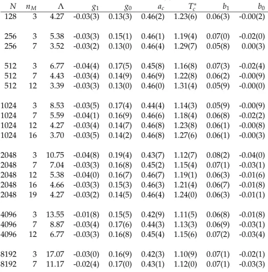
Landau Parameters
We report here the Landau parameters obtained with the variational en- hanced sampling method, as described in the main text. The parameters in Tab. 2.2 are obtained with a linear fit of the optimized parameters at tem- peratures
T = { 1.05, 1.10, 1.15, 1.20, 1.25, 1.30, 1.35, 1.40, 1.45, 1.50 } . (2.25) The lowest temperature for the fit is chosen in such a way that a good con- vergence is ensured at any T even for the bigger systems. Given Ginzburg- Landau free energy, Eq. (2.10), the fitting parameters are defined as follows:
g ( T ) = g
1T + g
0(2.26)
a ( T ) = a
c( T − T
c∗) (2.27)
b ( T ) = b
1T + b
0. (2.28)
Table 2.2:
Landau parameters for different systems sizes
Nand wave vector cutoff orders
nM. We recall that the coarse-grained length is
Λ=
N1/3/(
ρ1/30√
nM
) , and that in the thermodynamic limit the critical temperature is
Tc=
1.08(
5) .
N n
MΛ g
1g
0a
cT
c∗b
1b
0128 3 4.27 -0.03(3) 0.13(3) 0.46(2) 1.23(6) 0.06(3) -0.00(2) 256 3 5.38 -0.03(3) 0.15(1) 0.46(1) 1.19(4) 0.07(0) -0.02(0) 256 7 3.52 -0.03(2) 0.13(0) 0.46(4) 1.29(7) 0.05(8) 0.00(3) 512 3 6.77 -0.04(4) 0.17(5) 0.45(8) 1.16(8) 0.07(3) -0.02(4) 512 7 4.43 -0.03(4) 0.14(9) 0.46(9) 1.22(8) 0.06(2) -0.00(9) 512 12 3.39 -0.03(3) 0.13(0) 0.46(0) 1.31(4) 0.05(9) -0.00(0) 1024 3 8.53 -0.03(5) 0.17(4) 0.44(4) 1.14(3) 0.05(9) -0.00(9) 1024 7 5.59 -0.04(1) 0.16(9) 0.46(6) 1.18(4) 0.06(8) -0.02(2) 1024 12 4.27 -0.03(4) 0.14(7) 0.46(8) 1.23(8) 0.06(1) -0.00(8) 1024 16 3.70 -0.03(5) 0.14(2) 0.46(8) 1.27(6) 0.06(1) -0.00(3) 2048 3 10.75 -0.04(8) 0.19(4) 0.43(7) 1.12(7) 0.08(2) -0.04(0) 2048 7 7.04 -0.03(3) 0.16(8) 0.45(2) 1.15(4) 0.07(1) -0.03(1) 2048 12 5.38 -0.04(0) 0.16(7) 0.46(7) 1.19(1) 0.06(3) -0.01(6) 2048 16 4.66 -0.03(3) 0.15(3) 0.46(3) 1.21(4) 0.06(7) -0.01(8) 2048 19 4.27 -0.03(2) 0.14(5) 0.46(4) 1.24(0) 0.06(3) -0.01(1) 4096 3 13.55 -0.01(8) 0.15(5) 0.42(9) 1.11(5) 0.06(8) -0.01(8) 4096 7 8.87 -0.03(4) 0.17(6) 0.44(3) 1.13(3) 0.06(9) -0.03(1) 4096 12 6.77 -0.03(3) 0.16(8) 0.45(4) 1.15(6) 0.07(2) -0.03(4) 8192 3 17.07 -0.03(0) 0.16(9) 0.42(3) 1.10(9) 0.07(1) -0.02(1) 8192 7 11.17 -0.02(4) 0.17(0) 0.43(1) 1.12(0) 0.07(1) -0.03(3) The errors in our estimate of the GL parameters arise from two sources:
the statistical error coming from the stochastic optimization, and the error
provided by the linear fit. The former is significantly smaller than the fit
error.
2.2 Making the best of a bad situation: a multiscale approach to free energy calculation
This article, as the previous one, is based on VES and it is not directly con- nected to the OPES method. However, the paper discusses many of the key concepts that have been at the center of OPES development. Here we suggest the idea that the collective variables typically used in applications are almost always suboptimal and any enhanced sampling method should take into account the resulting multiscale behavior. For example, we argue that when dealing with suboptimal CVs, using a quasi-static bias is more important than having it to precisely reach convergence and fill in all the de- tails of the free energy surface. Thus the proposed method aims to achieve as quickly as possible an adiabatic regimen for the bias potential, which should then be modified only gently, allowing a reweighing procedure not affected by systematic errors to accurately retrieve the free energy and other observables. The OPES method adopts this same biasing strategy. Finally here we write the bias in such a way that it only depends on the free-energy difference between the basins, and thus the parameter to be optimize is ex- actly the physical quantity we are mostly interested into, as it will be the case in OPES when targeting expanded ensembles, Sec. 2.4.
My contribution to this article has been implementing the algorithms, per- forming the simulations, and writing the paper jointly with Prof. Parrinello.
Reference: M. Invernizzi, and M. Parrinello. “Making the best of a bad sit- uation: a multiscale approach to free energy calculation.” Journal of chemical theory and computation 15.4 (2019): 2187-2194. URL https://pubs.acs.org/
doi/10.1021/acs.jctc.9b00032
Copyright © 2019 American Chemical Society.
Making the Best of a Bad Situation: A Multiscale Approach to Free Energy Calculation
Michele Invernizzi*
1,2, and Michele Parrinello
3,21
Department of Physics, ETH Zurich c/o Universit`a della Svizzera italiana, 6900 Lugano, Switzerland
2
Facolt`a di Informatica, Institute of Computational Science, and National Center for Computational Design and Discovery of Novel Materials (MARVEL), Universit`a della
Svizzera italiana, 6900 Lugano, Switzerland
3
Department of Chemistry and Applied Biosciences, ETH Zurich c/o Universit`a della Svizzera italiana, 6900 Lugano, Switzerland
Abstract
Many enhanced sampling techniques rely on the identification of a number of collective variables that describe all the slow modes of the system. By constructing a bias potential in this reduced space, one is then able to sample efficiently and reconstruct the free energy land- scape. In methods such as metadynamics, the quality of these collective variables plays a key role in convergence efficiency. Unfortunately in many systems of interest it is not possible to identify an optimal col- lective variable, and one must deal with the nonideal situation of a system in which some slow modes are not accelerated. We propose a two-step approach in which, by taking into account the residual multi- scale nature of the problem, one is able to significantly speed up con- vergence. To do so, we combine an exploratory metadynamics run with an optimization of the free energy difference between metastable states, based on the recently proposed variationally enhanced sampling method. This new method is well parallelizable and is especially suited for complex systems, because of its simplicity and clear underlying physical picture.
2.2.1 Introduction
Many systems are characterized by metastable states separated by kinetic bottlenecks. Examples of this class of phenomena are chemical reactions, first order phase transitions, and protein folding. Calculating the difference in free energy between these states is of great importance, and various meth- ods have been developed to reach this goal [42, 43]. In this work, we focus on the case in which only two states are relevant. The generalization to a multistate scenario is not too difficult and will be discussed in a future publication.
In the two-state case one can distinguish two time scales, a shorter one in
which the system undergoes fluctuations while remaining in one of the min-
ima, and a longer one in which the system moves from one minimum to
another. This is the so-called rare event scenario, in which the separation
between the two time scales can be so large as to be inaccessible to direct molecular dynamics simulation, preventing a direct calculation of the free energy surface (FES).
In order to address this issue, a widely used class of free energy methods, including, among others, umbrella sampling [2], metadynamics [3] (MetaD), and variationally enhanced sampling [5, 44] (VES), aim at closing this time scale gap by speeding up the sampling of the slow modes of the system. To achieve this result, one first identifies a set of order parameters or collective variables (CVs) that are functions of the atomic coordinates s = s ( R ) . The CVs describe the slow modes whose sampling is accelerated by means of an applied bias potential V ( s ) . An optimal CV is such that if employed for an enhanced simulation run, it closes the time scale gap, so that intrastate and interstates exploration take place on the same time scale. A more common scenario is that the CV does not encode some slow modes, and although much reduced, the gap remains also in the enhanced sampling run. We shall refer to such CV as suboptimal. The limiting case would be that of a CV so poorly chosen that the gap falls outside the computational reach. In this case the CV would be not just suboptimal but also a bad CV. Given the crucial role of CVs, much effort has been devoted to their design and their systematic improvement [45–50].
In metadynamics and variationally enhanced sampling the effect of subopti- mal CVs manifests itself in a hysteretic behavior, easily detectable in the CV evolution. In these cases MetaD and VES efficiency suffers [20, 51–53]. The exploration of the system is still enhanced, and the calculation does even- tually converge [54], but this can require a substantial computational effort because, even after depositing the bias, some slow modes are present and the system retains a multiscale nature, with two separate time scales. More in detail, in this case the shape of the free energy surface in the basins is easily reconstructed, while their relative height is much harder to converge.
On the basis of this observation, we propose a multiscale approach that separates the calculation in two steps and aims at improving efficiency in a suboptimal CV scenario. First we reconstruct separately the free energy profile of each basin, using MetaD. In a second step we use the properties of VES to optimize their free energy difference and finally reconstruct the global FES. The purpose of our approach is to take into consideration the multiscale nature of a suboptimally enhanced simulation to speed up con- vergence.
First we shortly present to the unfamiliar reader MetaD and VES, and we
introduce a simple illustrative model that is helpful in visualizing the prob-
lem; then we explain in detail the proposed method. Finally we successfully
apply the new method to some representative systems.
2.2.2 Metadynamics and Variationally Enhanced Sampling
In this section we recall briefly the main features of the MetaD and VES meth- ods, both used in our approach. For a more in-depth review see e.g. Ref. [20].
Both methods enhance sampling by building on the fly a bias potential that is a function of a few collective variables. This bias discourages the system from remaining trapped in a metastable basin and forces it to explore other regions. It also provides an estimate of the free energy, which is related to the probability distribution:
e
−βF(s)Z = P ( s ) ∝
Z
dR e
−βU(R)δ [ s − s ( R )] , (2.29) Z = R
dse
−βF(s)being the normalization partition function, U ( R ) the poten- tial energy, and β = 1/ ( k
BT ) .
Metadynamics builds its bias as a sum of Gaussian contributions deposited periodically. In particular we will use its well-tempered variant (WTMetaD) [55], in which the height of the deposited Gaussian decreases exponentially as the bias is deposited:
V
n( s ) =
∑
n k=1G ( s, s
k) e
−β/(γ−1)Vk−1(sk), (2.30) where G ( s, s
k) = We
−ks−skk2is a Gaussian centered in s
k, the CVs value at time t
k. Independently from the choice of the Gaussian kernel parameters, this bias converges in the asymptotic limit to
V ( s ) = −( 1 − 1/γ ) F ( s ) + c , (2.31) where F ( s ) is the FES and c = c ( t ) does not depend on s. Once at conver- gence, the biased ensemble distribution P
V( s ) ∝ e
−β[F(s)+V(s)]is a smoother version of the unbiased one, i.e.: P
V( s ) = [ P ( s )]
1/γ. This broadening is controlled by the bias factor γ, which can go from 1 (unbiased case) up to infinity (non-well-tempered MetaD).
In the VES method, on the other hand, the bias is obtained as the result of the minimization of a convex functional:
Ω [ V ] = 1 β log
R ds e
−β[F(s)+V(s)]R ds e
−βF(s)+
Z
ds p ( s ) V ( s ) , (2.32) where p ( s ) is an arbitrary probability distribution called target distribution.
The VES functional is related to the relative entropy, or Kullback-Leibler divergence [56]. The minimum condition is reached when P
V( s ) = p ( s ) , a relation that can also be written as
F ( s ) = − V ( s ) − 1
β log p ( s ) . (2.33)
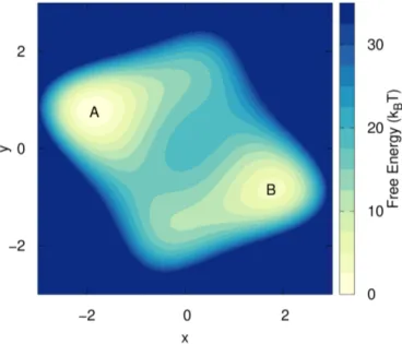
Figure 2.6:
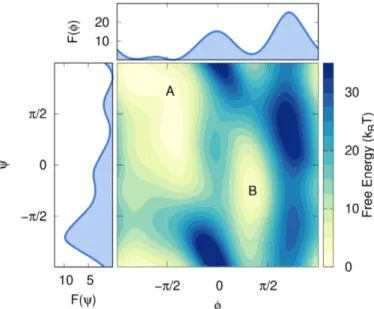
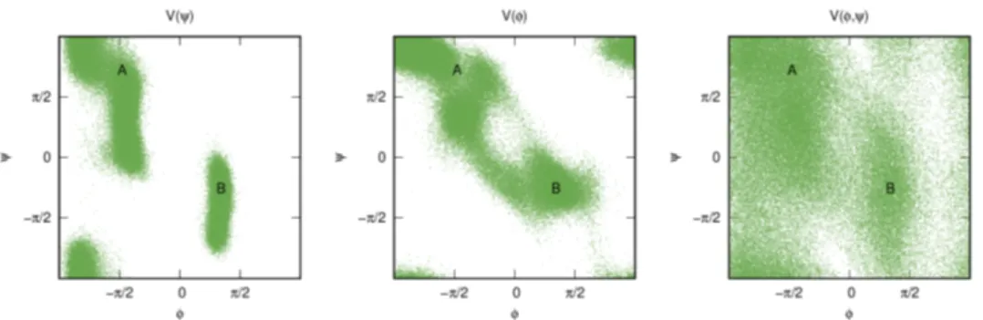
2D free energy surface of the considered model, with the two basins
Aand
B.It is possible to choose as target distribution the well-tempered one, p ( s ) = [ P ( s )]
1/γ. In this case the target has to be self-consistently adjusted as shown in Ref. [21]. At convergence one obtains the same bias potential as WT- MetaD.
In order to carry out the minimization of Ω [ V ] , the bias is usually expanded over an orthogonal basis set V ( s ) = ∑
kα
kf
k( s ) , or parametrized according to some physically motivated FES model [23, 26, 56]. In this way the functional becomes a function of the variational parameters and can be minimized using a stochastic gradient descent algorithm as described in Ref. [5].
2.2.3 Illustrative Model
In order to better acquaint the reader with the problem described in the in-
troduction (Sec. 2.2.1), we illustrate the phenomenology associated with the
use of suboptimal CVs in a simple model. The model consists of a single
particle moving with a Langevin dynamics on a 2D potential energy surface
(see Fig. 2.6) with two metastable basins, A and B, such that transitions be-
tween them are rare. This system has only two degrees of freedom, namely
the x and y positions. If we take x as CV and perform a well-tempered
MetaD run (details in the Supporting Information (SI), Sec. 2.2.7), we obtain
the result in Fig. 2.7. The fact that we are missing one degree of freedom can
be seen from the hysteresis apparent in the CV time evolution. In order to
go from one basin to the other, one must wait for a rare y fluctuation, result-
ing in a delay that cannot be enhanced by adding a bias on x. Nevertheless,
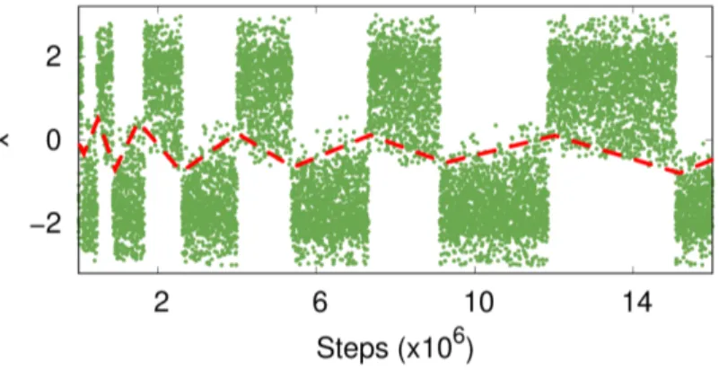
Figure 2.7:
Typical trajectory of a suboptimal CV, obtained via a WTMetaD run (γ =
10).Hysteresis can clearly be seen (highlighted by the red dashed line), and it is also visible how WTMetaD slowly reduces it, by depositing less bias as the simulation proceeds. While it is not possible to draw an horizontal line that separates the two basins, one can easily determine the basin of belonging for each point by inspecting the CV time evolution.
if we put more bias in one basin we open some higher pathways and tran- sitions are observed. However, they do not generally follow the lowest free energy path. This extra bias will also prevent the system from coming back to the same basin until it is properly compensated as the MetaD simulation progresses, and this gives rise to hysteresis.
Well-tempering reduces the amount of bias deposited in such a way that the hysteresis will eventually disappear, and in the asymptotic limit the bias will converge [54].
If we monitor the time dependence of the bias V ( x ) , we can see how the shape of the two basins is learned after just the first few transitions and remains pretty much unchanged throughout the simulation. After this quick initial phase, the vast majority of the computational effort is used to pin down the free energy difference ∆ F between the two basins.
2.2.4 Method
The observations made earlier suggest a two-step strategy. First one obtains the shape of the free energy surface in the different metastable basins, then optimizes the free energy difference between them. We will refer to this two-step procedure as VES∆F.
Free Energy Surface Model
In a rare event scenario, such as the one discussed in Sec. 2.2.3, there are
by definition distinct metastable basins and it is thus possible to identify
their separate contribution to the global FES. Formally this can be done by
considering the conditional probability P ( s | A ) , i.e., the probability that the CVs have value s when the system is in basin A.
P ( s | A ) ∝
Z
A
dR e
−βU(R)δ [ s − s ( R )] . (2.34) From P ( s | A ) one then can write an associated free energy:
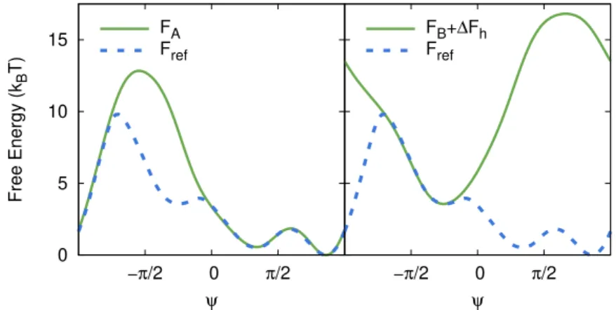
e
−βFA(s)Z
A= P ( s | A ) , (2.35)
where Z
Ais a normalization constant. With an identical procedure one can define F
B( s | B ) .
Notice that in general these probabilities are not mutually exclusive and, especially in the case of suboptimal CVs, there can be an overlapping region between them (see Fig. 2.7).
The global probability distribution is then obtained simply by combining these conditional probabilities:
P ( s ) = P ( s | A ) P
A+ P ( s | B ) P
B, (2.36) and the global free energy (modulo a constant) can thus be written as
F ( s ) = − 1 β log
"
e
−βFA(s)Z
A+ e
−βFB(s)
Z
Be
−β∆F#
, (2.37)
where the free energy difference between the basins ∆F is defined by e
−β∆F= P
BP
A= R
B
dR e
−βU(R)R
A