JulianWalter PartiellesZoomeningroßenNetzwerkgraphen Praktikumsbericht

(1)

Praktikumsbericht

Partielles Zoomen in großen Netzwerkgraphen

Julian Walter

Abgabedatum: 21. September 2019 Betreuer: Prof. Dr. Alexander Wolff

Johannes Zink M.Sc.

Dr. David Hock Fabian Lipp M.Sc.

Julius-Maximilians-Universität Würzburg Lehrstuhl für Informatik I

Algorithmen, Komplexität und wissensbasierte Systeme

(2)

Zusammenfassung

Dieser Praktikumsbericht befasst sich mit Möglichkeiten zum partiellen Zoomen in Netz- werkgraphen. Im Rahmen des zugehörigen Praktikums wurden Ideen für Algorithmen hierzu und mögliche Visualisierungsvarianten gesammelt und verglichen. Hiervon wurde eine Variante ausgewählt und mit Hilfe der Programmbibliothek yFiles implementiert.

(3)

Inhaltsverzeichnis

1 Einleitung 4

2 Literaturüberblick 6

3 Visualisierung 13

3.1 Zoomen, dann clustern . . . 13

3.2 Hierarchisches Fisheye . . . 15

3.3 Fokusbereich + Randbereich . . . 16

3.4 Ebenen durch Rahmen . . . 18

3.5 Fokusebene + Verbindungsknoten . . . 19

3.6 Zu allen Ansätzen . . . 21

4 Umsetzung 22 4.1 Änderung der sichtbaren Knoten . . . 22

4.2 Änderung der sichtbaren Kanten . . . 23

4.3 Visualisierung . . . 24

4.4 Tests . . . 25

5 Ausblick 27

3

(4)

1 Einleitung

Ziel der Arbeit ist es, einen Algorithmus zum partiellen Zoomen – ähnlich einer Fisheye- Ansicht – in einen großen Graphen zu entwickeln und zu implementieren. In der Fotografie wird mit einem Fisheye-Objektiv ein großer Bereich abgebildet – meist180^◦-Ansichten.

Hierbei wird der mittlere Bereich, welcher im Fokus ist, nahezu unverzerrt dargestellt und das Bild zu den Seiten hin gestaucht um den großen Bereich abbilden zu können.

Angewendet auf einem Graphen kann das beispielsweise bedeuten, den fokussierten Be- reich übersichtlich und detailliert zu halten und die Randbereiche zu stauchen oder zu clustern. Hintergrund war die Überlegung, einen Graphen zu visualisieren, welcher das komplette IT-Netzwerk eines Unternehmens beinhaltet, also alle Rechner und deren Ver- kabelung. Bei global agierenden Unternehmen kann das allein für einen Standort schon weit mehr Knoten und Kanten bedeuten, als auf einem 1080p-Display oder einer DIN A4-Seite übersichtlich dargestellt werden können.

Hierbei war der Wunsch, eine Möglichkeit zu finden, in Teile des Graphen hineinzoo- men zu können, wobei jederzeit der komplette Graph zur Orientierung sichtbar bleibt.

Der Gedanke dahinter ist, dass sich die „mental map“ des Benutzers beim Zoomen er- hält. Damit zusammenhängend ist das Problem des Clusterns der Knoten, wobei auch Attribute von Knoten oder Kanten eine Rolle spielen können, welche vom Benutzer fest- gelegt sein können. Der Benutzer sollte angeben können, wie weit er einen Superknoten oder eine Teilmenge von Knoten vergrößern oder verkleinern möchte. Dies soll durch die Repräsentation von Teilen des Graphen durch einzelne Knoten – wie z. B. einen Knoten, repräsentativ für Europa, während ein Standort in den USA näher betrachtet wird – oder eine passend beschriftete, aus dem angezeigten Bereich herausführende Kante er- reicht werden. Eine weitere Option für den Nutzer könnte ein „Knoten-Klick“ darstellen, wobei beim Klick auf einen Superknoten dieser ausgeklappt und auf dessen Unterknoten gezoomt wird.

Ebenfalls ist es wichtig darauf zu achten, dass die Gesamtmenge der sichtbaren Knoten nicht zu groß wird, um die Übersichtlichkeit zu gewährleisten. Hierzu könnte beispielsweise ein Schwellwert eingeführt werden; wird dieser beim Ausklappen eines Knotens überschritten, müssen am Rand Knoten zusammengefasst werden. Der Maßstab soll sich also beim Zoomen nicht gleichmäßig auf dem ganzen Graphen verändern, stattdessen sollten die wichtigen Gebiete zulasten der unwichtigen vergrößert bzw. detaillierter dargestellt werden.

Spezifizierung der Aufgabenstellung. Die Aufgabe des Praktikums bestand im Finden und Implementieren eines Algorithmus, welcher bei Eingabe eines großen Graphen eine übersichtliche Darstellung dieses Graphen durch Zusammenfassen der Knoten des nicht fokussierten Bereichs zu Clustern berechnet. Ein großer Graph bedeutet hier, ein Graph mit mehr Knoten als übersichtlich auf einem 1080p-Display oder auf einer DIN A4 Seite dargestellt werden können. Eine übersichtliche Darstellung beinhaltet, dass einzelne Kno- ten und Kanten mit bloßem Auge eindeutig identifiziert werden können und genügend Platz für eine lesbare Beschriftung vorhanden ist.

(5)

Übersicht. In Abschnitt 2 „Literaturüberblick“ werden einige Paper vorgestellt, welche sich mit diesem Thema auseinandersetzen. Abschnitt 3 „Visualisierung“ beschäftigt sich mit Möglichkeiten der Darstellung des Zoomens – dazu zählen unter anderem die Re- präsentation der zusammengefassten Knoten und Übergangsanimationen. In Abschnitt 4

„Umsetzung“ ist die Implementierung des ausgewählten Modells näher beschrieben. In Abschnitt 5 „Ausblick“ werden Ideen vorgestellt, wie auf diese Arbeit aufgebaut werden kann.

5

(6)

2 Literaturüberblick

Tominski et al. befassen sich in ihrem Paper „Fisheye Tree Views and Lenses for Graph Visualization“ [TAVHS06] damit, wie ein Teilbereich eines großen Graphen durch Zoomen übersichtlich dargestellt werden kann. Hierzu haben sich die Autoren mit unterschiedlichen Lupenfunktionen auseinandergesetzt, welche jeweils den fokussierten Bereich auf un- terschiedliche Art und Weise übersichtlicher darzustellen versuchen. Diese sind die „Local Edge Lens“, die „Bring Neighbors Lens“ und eine „Composite Lens“, welche beide anderen Lupenfunktionen und zusätzlich gleichzeitig eine traditionelle Fisheye-Lupenfunktion bereitstellt.

Zu sehen ist deren Wirkungsweise am besten in der Graphik aus ihrem Paper, welche in Abbildung 1 zu sehen ist. Abbildung 1b zeigt die „Local Edge Lens“, die alle Kanten, welche den fokussierten Bereich schneiden, ausblendet. Nur Kanten, welche von und zu Knoten innerhalb des fokussierten Bereichs führen, werden angezeigt. Die „Bring Neigh- bors Lens“, zu sehen in Abbildung 1c verschiebt temporär alle Endknoten von Kanten, welche aus dem fokussierten Bereich heraus führen, in den fokussierten Bereich hinein.

In Abbildung 1d ist die „Composite Lens“ dargestellt, welche die beiden anderen Lupen- funktionen und die Fisheye-Ansicht kombiniert.

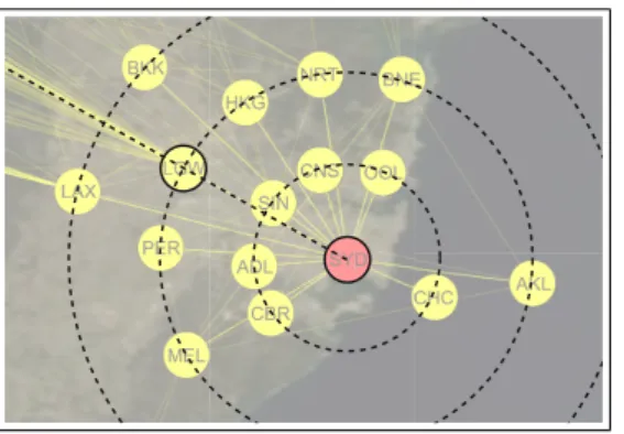
Eine andere Variante „Bring Neighbors Lens“ wird in dem Paper „Topology-Aware Navigation in Large Networks“ [MCH⁺09] von Moscovich et al. vorgestellt. Deren Lu- penfunktion nennt sich „Bring & Go“, zu sehen in Abbildung 2, welche eine Graphik von Moscovich et al. zeigt. Hier ist die „Bring & Go“-Funktion am Beispiel von Flügen von und nach Sydney visualisiert. Die anderen Start- bzw. Zielflughäfen werden in den Bereich um Sydney herum zusammen gezogen. Diese Funktion unterscheidet sich von der „Bring Neighbors Lens“ dahingehend, dass hier die Knoten auf festen Radien um den Fokusknoten herum angeordnet werden, welche gleichzeitig den relativen Abstand zeigen (zu sehen in Abbildung 3). Flughäfen, welche sehr weit von Sydney entfernt liegen, werden auf den äußersten Ring verlegt, während Knoten, welche Flughäfen nahe Sydney repräsentieren auf den innersten Ring gezeichnet werden.

Eine Übersicht über einige ähnliche Arbeiten, wie die zwei bereits hier vorgestellten, wurde von Tominski et al. in deren Artikel „A Survey on Interactive Lenses in Visualiza- tion“ [TGK⁺14] zusammengetragen. In diesem sind einige weitere Arbeiten vorgestellt, welche sich mit unterschiedlichen Lupenfunktionen befassen.

Eine andere, verbreitete Herangehensweise ist, zu versuchen den Graphen in Cluster zu unterteilen und durch Nutzung dieser Informationen den gesamten Graphen übersichtli- cher darzustellen. Hierzu gibt es Arbeiten wie „Large Graph Visualization by Hierarchi- cal Clustering“ [HN08] von Huang und Nguyen, die klassisch die Knoten clustern sowie Arbeiten wie „Geometry-Based Edge Clustering for Graph Visualization“[CZQ⁺08] von Cui et al. welche sich mit dem Zusammenfassen von Kanten beschäftigen, um den Graph übersichtlicher zu machen.

In ihrem Paper „Interactive Visualization of Small World Graphs“ [VHVW04] haben sich die Autoren Frank van Ham und Jarke J. van Wijk mit dem Problem der dreidimen- sionalen Darstellung eines Graphen befasst, der zu groß ist um ihn übersichtlich mit allen Knoten und Kanten zu visualisieren. Ihre Herangehensweise lässt sich aber unverändert

(7)

5. Conclusion and discussion

In this paper we have addressed aspects related to the navigation and visual exploration of graph structures. An adequate visual interface for this task must provide different interactive views that allow one to easily navigate the visualized structures and to intuitively explore large graph data according to different aspects.

We described Textual and Non-Textual Fisheye Tree Views as visual interfaces to trees. The simplicity of these interfaces opens up the possibility of using them for a variety of daily tasks. The presented interaction methods, specifically the on-demand 1D fisheye transformation, provide support for more complicated visualization tasks.

This is achieved by incorporating overview+detail and focus+context concepts in an integrated fashion.

As a second contribution of this paper, we have exemplified the usefulness of lens techniques for displaying, on demand, local information that may be otherwise difficult to grasp in large and dense graph layouts. While the Local Edge Lens is a lens that supports the detection of edges within the lens scope, the Bring Neighbors Lens is a tool to bring in neighboring vertices of the vertices within the lens perimeter. The developed Local Edge Lens and the novel Bring Neighbors Lens have been combined with a fisheye lens to illustrate the composition of different lens types. By this composition,

the advantages of the original lenses can be accommodated in one advanced lens.

The described methods have been incorporated in a framework for visualizing clustered graphs. We are currently evaluating and tuning the proposed methods for the exploration and navigation of clustered graphs with up to 100,000 vertices.

Although initial user tests have been conducted, which led to the development of the Composite Lens, it is necessary to further evaluate the proposed visual interfaces and interaction techniques with concrete observable graph exploration tasks. Among the concerns that surfaced in the initial user test were the coordination of the different views and the consistency of interaction among the different techniques. These will be addressed in future work. Further user tests could also lead to a demand for additional views or new lens techniques.

Another interesting issue to investigate in the future is to develop a generalized model for integrating lenses at the different stages of the visualization pipeline.

6. Acknowledgements

Special thanks go to Konrad Borys for his advice regarding the Bring Neighbors Lens. The support provided by the DIMACS center at Rutgers University for this project is gratefully acknowledged.

(a)

(c) (d)

(b)

Figure 7: The figure provides a comparative view of the presented lens types. (a) No lens; (b) Local Edge Lens; (c) Bring Neighbors Lens; (d) Composite Lens which integrates (b) and (c) as well as an

additional fisheye lens.

(a)Ausschnitt ohne Lupe

(a)

(c) (d)

(b)

(b) „Local Edge Lens“

(a)

(c) (d)

(b)

(c)„Bring Neighbors Lens“

(a)

(c) (d)

(b)

(d) „Composite Lens“

Abb. 1: Graphiken aus dem Paper „Fisheye Tree Views and Lenses for Graph Visualization“

[TAVHS06]; Auswirkungen der verschiedenen vorgestellten Lupen am Ausschnitt eines Beispielgraphen

furthest neighbor edges to bundle

furthest node edges to bundle

junction node

Figure 3. Multiple links leaving a node in the same compass direction (a) are collected into bundles by routing them through a dummy junction node (b). The process is repeated until the number of bundles leaving all nodes or junctions in the same compass direction fall below a given threshold (c).

(a) (b) (c)

Figure 4. (a) Highlighting all flights to/from Sydney, Australia. (b) Close-up on Sydney, with highlighting. (c) Bring & Go initiated on Sydney.

BRING & GO

Link Sliding makes it easy to navigate along a given path.

However, it does not help in the decision process that leads to the selection of one path among many potential candidates.

This decision might depend on the type of arc to be followed when there are different types of paths. It might also depend on attributes of the node at the other end of the path. Having to navigate to the other end, in order to decide whether this is the path of interest or not, quickly becomes tedious as the number of connected arcs increases.

Bring & Go addresses this problem by bringing adjacent nodes close to a node upon selection. Figure 4-a shows a map of about 700 commercial flights connecting 232 airports. Highlighting (in red) gives a general idea of the number and location of airports connected to the currently selected node: Sydney International. At this scale, the node is difficult to select, being only 1-pixel large on a 17” display.

Moreover, some parts of the network are very crowded, mak- ing it difficult to visually follow the paths. One has to zoom- in to get detailed information such as airport names, thus losing context and moving all airports connected to Syd- ney out of the viewport (Figure 4-b). When selecting the node corresponding to Sydney, Bring & Go translates all airports connected to it inside the current viewport (Figure 4-c) using smooth animations to preserve perceptual continuity [29]. The spline curves that represent links are smoothly flattened and brought inside the viewport, thus providing additional contextual information, such as the degree of connected nodes, that might help the user make his decision.

For instance, the user might be looking firstly for an airport hub, which would be more likely to offer him a direct flight to his final destination.

Once the user has made a decision about what link to follow, Bring & Go makes it very easy to reach the corresponding node with a simple selection of that node. The viewport is smoothly animated, zooming out and then in to get some context, as when traveling along a path with Link Sliding (see section on distance-dependent automatic zooming for details about the computation of the trajectory in space and scale). In the meantime, all nodes and splines are animated back to their previous position and geometry, thus restoring the network to its original configuration and terminating the Bring & Go.

The concept of Bring & Go is similar to Hopping [18] and Drag-and-Pop[3], which facilitate selection by bringing prox- ies of potential targets closer to the cursor. Bring & Go, however, is designed for navigation, rather than selection, and can handle a much larger number of distant targets, as only connected nodes are brought close. The technique is also similar to the Bring Neighbors Lens [31], which ad- justs the layout of the graph to bring connected nodes into view. However, we believe that Bring & Go’s use of prox- ies, rather than distortion, better preserves spatial constancy, and is critical for geographically embedded networks. Most importantly, Bring & Go works iteratively: a new Bring &

Go can be initiated on a node that is currently inside the viewport as the result of a previous Bring & Go, bringing additional nodes into view, and so on. Looking for a flight from Sydney to Tel Aviv (which are not directly connected in our network), a user would easily identify London as a hub and, thanks to a second Bring & Go initiated on the London node brought inside the viewport, find that it is connected to Tel Aviv.

(a) Gesamte Weltkarte

junction node

(a) (b) (c)

BRING & GO

(b)Ausschnitt ohne Lupe

junction node

(a) (b) (c)

BRING & GO

(c) mit „Bring & Go“

Abb. 2: Graphiken aus dem Paper „Topology-Aware Navigation in Large Networks“ [MCH⁺09];

Beispiel eines Graphen welcher Flugrouten repräsentiert; „Bring & Go“-Funktion am Beispiel des Kartenausschnitts Sydney

7

(8)

Bring & Go Layout

The layout algorithm for computing the position of nodes brought inside the viewport is relatively simple. As illus- trated in Figure 5, nodes are placed in concentric circles centered on the selected node according to the following method.

Polar coordinates (ρ, θ) are computed for all connected nodes.

The list of nodes to be brought inside the viewport is sorted by distanceρ(shortest first). Nodes are then brought onto the rings following this order. For each node the algorithm checks each ring, starting from the innermost one, until it finds one where the node can be laid out, without overlapping any previously laid-out node, while keeping itsθcoor- dinate constant. This method preserves the direction to the original location of brought nodes, and gives a sense of their relative distance to the selected node.

Figure 5. The layout of brought nodes preserves the direction to their actual location, and gives a sense of their relative distance to the selected node.

EXPERIMENT

We conducted an experiment to compare the performance and limits of Bring & Go (hereafter abbreviated B&G) and Link Sliding (LS) with simple visual augmentation of the methods currently available for navigating in node-link dia- grams: Pan & Zoom (PZ), and interactive Bird’s Eye View (BEV). Participants were asked to perform a compound navigation task on an abstract graph. We measured the performance time for each sub-task, and accuracy where relevant.

Following the task participants responded to a questionnaire regarding their experience.

Task and Stimuli

All navigation tasks are set in one of two randomly generated scale-free graphs, onesparse, and onedense. The graphs were created using a Bar´abasi-Albert model [2]. In the graph generation process, each new node is connected to ndistinct nodes, randomly chosen from the existing nodes.

Thesparse graph(1000 nodes, 1485 edges) was generated with a random connectivityn∈[1,2], and thedense graph (1000 nodes, 2488 edges) usingn∈[1,5]. We also provide a small graph (200 nodes, 477 edges) for training purposes.

The nodes on the graphs are labeled with the names of an- imals, and vegetables. Unlike a real-world task, where the node labels are meaningful to the user, random name labels can be difficult to remember. To reduce the cognitive load on our participants we consistently give the start node the label

“rat”, and give one of its neighbors the label “cat” (explained below).

The trials in each condition are assigned to four fixed patterns in the corresponding graph, each consisting of a starting node and its neighbors. A pattern has a starting node of degreed(d= 5in thesparsegraph, andd= 10in thedense graph). For each technique, participants perform timed tasks for all patterns of the two graphs. As we have four techniques, we provided four versions of each graph: the initial one, and its rotations by 90, 180 and 260 degrees. The labels are changed for each graph pattern, but retain their animal/vegetable category.

As each technique we study may be best suited to a different graph navigation tasks, we select three representative task from Leeet al.’s task taxonomy for graph visualization [22].

The tasks include identifying all nodes connected to a given node, following a link, and returning to a previously visited link. Participants performed the three tasks in sequence to complete one trial. The first task (neighborstask) is to identify a node’s immediate neighbors. Participants begin at the start node, which is highlighted in orange, and are asked to count how many of the node’s neighbors are labeled with an animal name, and to remember the location of the cat node.

Participants press the space-bar to start, and press it again when they are done counting. After typing in the number of animal nodes, the system informs the participant if they have counted correctly. In the second task (followtask), the system centers the view about the start node, and participants are asked to follow a link, highlighted in orange, from the start node to a selected “visit node”. Pressing the space-bar begins the task and clicking on the visit node completes it.

Participants are then instructed to begin the third task (revisit task). Participants press the space-bar to start, and must then locate the cat node that they have seen in theneighborstask, and click on it. They may do this either by retracing their steps back to the start node, or by moving directly to where they believe the cat node is located.

To control the tasks completion time, the sum of the distances between the starting node and its neighbors is constant in all trials of the sparse graph, and all trials of the dense graph. The distance between the starting node and the cat node is constant in all patterns, as is the distance between the starting node and the visit node. Participants were given a maximum of 40 seconds to perform each task.

Design

Our experiment follows a4×2within-subject design: each participant performs tasks using each of the four techniques (T echnique∈ {PZ, BEV, B&G, LS}) under two different graph conditions (G∈ {Sparse, Dense}). We group trials into four blocks, one per technique, so as not to confuse participants with frequent changes of the technique. To avoid

Abb. 3: „Bring & Go“ am Beispiel Sydney[MCH⁺09]; herangezogene Knoten werden auf festen Radien um den Sydney-Knoten herum angeordnet

auch im Zweidimensionalen anwenden; sie ist die Folgende: Zuerst werden alle Knoten des Graphen zu hierarchischen Clustern zusammengefasst. Danach wird der Graph nur mit den Superknoten, welche die größten Cluster repräsentieren, visualisiert. Für die De- tails wurde eine Art Lupe entworfen, genannt „fisheye lens“, welche eine Fisheye-Ansicht auf der Abstraktionsebene realisiert. Das bedeutet, dass Superknoten, die „unter die Lu- pe genommen werden“, entpackt werden und somit im mittleren Bereich der Lupe alle Knoten zu sehen sind. In einem festgelegten Gebiet um diesen Bereich steigt die Abstrak- tion nach außen hin an, sodass weiter innen kleinere Cluster niedrigerer Hierarchiestufen abgebildet sind, welche weniger Knoten repräsentieren, und nach außen hin immer grö- ßere. Außerhalb dieses Bereichs sind nur noch Superknoten der höchsten Hierarchiestufe dargestellt.

Der theoretische Aufbau dieser Bereiche ist in Abbildung 4b zu sehen. Der Fokuspunkt ist durch f markiert. Um ihn herum gibt es den hellblau markierten, inneren Bereich, gekennzeichnet durch den Buchstaben A, in welchem Knoten des ursprünglichen Gra- phen zu sehen sind. Danach kommt der ÜbergangsbereichB in welchem die Abstraktion ansteigt und nach außen hin immer mehr Knoten zu Clustern zusammengefasst werden.

Der Rest ist der Bereich C, in welchem ausschließlich Superknoten dargestellt sind.

Anschaulich dargestellt sind die Auswirkungen der „fisheye lens“ am Beispielgraphen in Abbildung 4a. Abbildung 4c zeigt, wie sich dieser Graph unter Verwendung der Lu- penfunktion bei unterschiedlichen Fokuspunkten verändert.

In vielen Arbeiten zum Thema Fisheye-Ansicht wird der Artikel „Generalized Fisheye Views“ [Fur86] von George W. Furnas zitiert. Auf dem darin vorgestellten Berechnungs- ansatz baut auch das Programm Semnet [FPF13] von Fairchild, Poltrock und Furnas auf, welches ebenfalls oft erwähnt wird. In seinem Artikel beschreibt Furnas zum einen ausführlich warum eine Fisheye-Ansicht sinnvoll ist und stellt dann eine Berechnung einer solchen Ansicht mithilfe des „Degree of Interest“ (DOI) vor. Der DOI ist ein Wert, der jedem Knoten zugeordnet wird. Je größer er ist, desto wichtiger ist der zugehörige Knoten für den Betrachter.

Zu sehen ist das ganze in Abbildung 5; hier ist die Berechnung des DOI am Beispiel eines Baumgraphen dargestellt. Die Berechnung ist simpel, es werden für jeden Knoten zwei

(9)

a b c

Figure 4: Using explicit clustering to abstract the graph: (a) Straight cut, (b) Semantic Fisheye using a cubic DOA function and (c) Semantic Fisheye with a linear DOA function integrated with a geometrical ﬁsheye

This resulted in layouts with a substantial smaller energy than the ones we obtained starting from a random initial positioning in the same number of iterations, as is shown in ﬁgure 2. To test whether the visual clusters generated by the layout algorithm, ac- tually correspond to semantical clusters in the dataset, we added expert data on a painters artistic movement (unfortunately we were unable to retrieve this information for all painters) and used it to color the nodes (Figure 2b). For all modern movements (right half) the image shows a clear coherence between the movement and the clustering in the layout. For most classical painters (left half) this coherence is much less clear however. Although we are able to ﬁnd some small structural clusters based on movement, we suspect that most pre-17th century artists are likely clustered based on another (unknown) property, such as geographical location.

4 VISUALIZATION

Given a layoutL_Gof a graphG, we can state that highly connected subgraphs are now visible as areas with a higher node density. How- ever, the image shown in ﬁgure 2(b) is still noisy and hard to read.

Apart from that, displaying all nodes and edges at one single time is simply not an option if when dealing with larger graphs. We have to provide a way to reduce the number of visible elements, while maintaining the global structure of the graph. In other words, we have to provide a visual abstraction ofL_G. At the same time the user will also be interested in details, so we have to ﬁnd an accept- able way to integrate detail with context. The visualization of edges also remains a problem, since the large number of long edges in the picture make it hard to trace individual connections. We discuss each of the problems mentioned above in the next sections

4.1 Visual Abstraction

A simple but effective way to provide visual abstraction without losing a sense of the global structure is to render the nodes as overlapping spheres with constant size in screen space. The result- ing conﬁguration of partly overlapping spheres visually abstracts a cluster of nodes, showing it as a blob like structure. At the same time, the internal structure of a cluster is still visible as a shaded Voronoi diagram, giving an impression on how the cluster falls apart when we zoom in. By keeping the screen size of nodes constant while zooming in on the structure, we obtain progressively more details. In fact, this method can be seen as a fast alternative to

[30], with the added ability to continuously display the graph at any level of abstraction by zooming in or out. Figure 3 shows our sam- ple graph at three zoom levels, nodes are colored based on birthdate.

For example, 16th century painter Guiseppe Arcimboldo is classi- ﬁed as (a very early) surrealist, which is not so strange considering his paintings.

Another often used way to provide abstraction is to compute a clustering onL_G. In the layout the distance between clusters is in- versely proportional to their coupling. This means that we can use the geometric distances between nodes as a useful clustering metric, since the most tightly coupled clusters are geometrically closest. We perform a bottom up agglomerative clustering onGusing any distance measured(i,j)between two clustersiandj. Deﬁne a clusterkas a tuple(c_k,r_k,d_k,f_k), wherec_krepresents the cluster’s center, r_k its radius, d_k the distance between its two subclusters and f_k its parent cluster. Initially we assign all nodesito separate clusters(p_i,r_base,0,nil). Next, we iteratively merge clusters by selecting the two clustersiand j with minimald(i,j)and merging them in a new cluster k. For all edgese_{(i j)x} incident toior jwe create a new edgee_kx. If an edgee_kxalready exists we increase its weight byw(e_{(i j)x}).

The new cluster has to provide some visual feedback on the amount of leaf nodes it contains and their approximate positions.

LetLN(k)be the set of leaf nodes in clusterk. A straightforward choice forc_kis the average position of all leaf nodesl∈LN(k). We let the radiusr_k depend on|LN(k)|. Linear (radius is proportional to size), a square root (area is proportional to size) or a cube root (area is proportional to volume) function are all candidates. We found that the square root function provides better results in general, since a linear function sometimes leads to excessively large clusters, while a cube root function makes it too hard to discern size differences.

This leaves us with choosing a suitable distance functiond(i,j) to determine the distance between two clusters. Widely used met- rics in clustering literature deﬁne the inter cluster distance as a function of the distances between their (leaf)members [14].

Well known variants are minimum link, maximum link and average link distance. Minimum link deﬁnes the distanced(i,j)between clustersiand jas the distance between the two closest members of both clusters, maximum link uses the distance between the 202

Authorized licensed use limited to: University of Calgary. Downloaded on January 22, 2009 at 16:08 from IEEE Xplore. Restrictions apply.

(a) Geclusterter Graph ohne Lupe

two furthest members, while average link uses the average distance between all members.

Clustering using the minimum link measure has the tendency to form long chains, while maximum link clustering is very sensi- tive to outliers. Average link clustering generally provides a good optimum between both and is our metric of choice here. For the distances between cluster members (i.e. the leaf nodes) we can choose either the geometric distance or the edge length, with the edge length between unconnected nodes set to inﬁnity. The latter method does not allow clusters that are not interconnected but po- sitioned geometrically close by a suboptimal layout to be merged.

Although aesthetically less pleasing, we use the edge lengths for clustering because it creates better clusters.

Applying the cluster algorithm outlined above results in abinary hierarchyor dendrogram, where the level in the hierarchy for a clusterkis equal to the distancedkbetween its child clusters. A simple way to create abstractions for a clustered graph is to deﬁne a globaldegree of abstraction DOA∈[0,1]and display only those clusterskfor whichdk≤droot·DOA<dfk(Figure 4.1). To create a continuous transition whenDOAis changed we can interpolate between the size and position of clusterkand the size and position of its parent cluster using a local parameterλkwhere

λk= ((DOA·droot)−dk)/(dfk−dk)

λkis a parameter that indicates the amount of interpolation between the position and size of a clusterkand the position and size of its parent fkbased on the degree of abstraction at that point. We can state that 0≤λk≤1 for all visible clusters, because dk≤droot·DOA<dfk.

Based on user preference we can either use linear, exponential or slow-in slow-out interpolation (Fig 5). We found a combination of a linear interpolation for the positions and an exponential interpolation for the cluster size to give the best results. Interpolating cluster sizes exponentially prevents small isolated clusters from growing to their parents size too quickly. Usingλwe can compute sizes and positions for all clusters visible in the current ’slice’ of the hierarchy and we can show the graph at an arbitrary level of detail by varying the DOA. Note that a similar idea was coined by [26], but their ’horizons’ are deﬁned on a hierarchy with discrete levels and the hierarchy is generated based on a simple recursive space subdivision technique that does not always generate very accurate clusters. The procedure outlined above is in effect a continuous version of this idea. Figure 4a shows our artists graph at a higher level of abstraction, representing a reduction of 97% in the number of visible nodes.

Figure 5: Interpolation of sizes and positions based on current DOA.

Linear interpolation on the left, exponential interpolation on the right

Figure 6: Top down view of visualization area indicating the three diﬀerent methods of visual abstraction: area A uses a ﬁsheye lens to distort node positions, area B incrementally abstracts nodes and area C displays nodes with a constant DOA to avoid unnecessary motion in the periphery

Figure 7: Schematic cross section, showing the cluster dendrogram with constant and variable DOA functions

4.2 Detail and Context

Providing both detailed information as well as a global context in one image is one of the fundamental problems in Information Vi- sualization. Although we are able to provide views of a graph at different levels of abstraction, the user will probably be more interested in obtaining detail information for some speciﬁc section of the graph. One solution is to embed this detail in the global graph structure in a useful way, allowing the user to maintain both a context for the local area he is interested in, as well as a consistent global mental map of the entire structure.

One often used way of embedding local detail in global context is the Fisheye View. Generalized Fisheye views [12] deﬁne a De- gree of Interest for an information element based on its a priori importance and its distance to a focal point. Most applications of the ﬁsheye technique fall into one of two categories. One are the distortion orientedtechniques, which distort the sizes and positions

203

(b)Bereiche der Lupenfunktion

Figure 8: Series of frames showing the eﬀect of a changing focus on the layout. Surrealist artists are indicated in red, artists belonging to the Pop-Art movement in green.

of nodes based on their geometric distance to the focus. This can be either done in the layout stage by employing a hyperbolic distance measure [18, 21] or as a successive projection step on an existing layout [28, 19, 6, 31]. The other aredata suppressiontechniques that hide or abstract nodes based on the distance to a focus, creating an abstracted layout. Although conceptually closer to Furnas’ original idea, relatively few researchers have pursued this path. Most notable are [9, 26], while others, such as [29] also use abstraction coupled with a distortion function but require the user to manually expand and collapse clusters of interest.

Distortion oriented techniques provide a local geometric zoom that is easily understandable, but still require all nodes to be drawn.

Data suppression techniques avoid this and only display a fraction of the nodes, but they require extra attention to keep the relation- ship between nodes and their abstractions understandable. Often used ways to do this are by visual containment (i.e. always displaying a node visually contained in its abstraction) or animation (by animating from an abstracted layout to a detailed layout). Since both techniques have their individual merits, we propose to integrate them in a single scheme (ﬁg 4c).

That is, we use a geometric ﬁsheye by varying the local zoom factor with the distance from a focus and a semantic ﬁsheye by varying the DOA with the distance from the focus. We therefore divide the visualization area into three concentric sections, based on the distancesof a pointpto a focal pointf(Figure 6) : A focal areaAwheres≤Rf, an areaBwithRf<s≤RDOAin which we increasingly abstract nodes and an areaCin which we keep the degree of abstraction constant.

For points within the focal areaAwe use a variable geometric zoom. We prefer a functionZthat magniﬁes sections close tofbut does not distort whens≥Rf. A suitable function is the Fisheye Distortion function from [28], i.e.,

Z(s) =_{z s/R}^(z+1)_f₊₁^s if s<Rf Z(s) =s if s≥Rf

In this casezis a factor that determines the amount of zoom near the focus. Instead of also scaling the node sizes, like a com- mon ﬁsheye lens does, we keep the size of nodes in screen space constant, analogous to the abstraction method mentioned at the be- ginning of the previous paragraph. This gives the visual effect that a tightly packed cluster of nodes gets ‘pulled apart’ near the center of the ﬁsheye lens.

For points outside the focal area we use a semantic ﬁsheye, that is, pointspfor whichRf<s≤RDOAare increasingly abstracted with increasing distance from the focus (areaB). In other words, instead of a single global abstraction levelDOA, we deﬁne a function

DOA(s)∈[0,1]that speciﬁes a degree of abstraction as a function of the distancesof a pointptof.

We then render the graph by only rendering the highest clusters in the hierarchykfor which

dk≤droot·DOA(|ck−f|)∧droot·DOA(|cfk−f|)<dfk

We can ﬁnd these clusters quickly by inspecting the hierarchy in a top-down fashion. We use a DOA function that does not abstract nodes in areaA, is increasing in areaBand has a constant value in areaC:

DOA(s) =0 if s<Rf DOA(s) =a(s) if Rf<s≤RDOA DOA(s) =a(RDOA) if RDOA<s

The choice of an increasing functionais arbitrary, but linear and cubic functions are straightforward choices here. Figure 4 shows samples of both. By using a constant DOA for nodes in areaC, we avoid changing the interpolated sizes and positions for these nodes when the focus changes. Since movement is such a strong visual cue, viewer attention might get distracted from the focal area to the context, which is undesirable. Figure 7 shows these concepts schematically.

Summarizing the above, a nodeiat distances=|pi−f|from the focus point is displayed by:

1.abstractingthe node based on a functionDOA(s).

2.projectingthe abstracted node at positionf+Z(s)·^pⁱ^−f_s . By visually indicating the edge of the ﬁsheye distortion, we make these two different zooming actions (one geometric and the other semantic) more understandable for the user (Fig 4c). The overall effect obtained when moving the focus bears a lot of resemblance to the Magic Lens [5]. Fig 8 shows a number of intermediate frames when moving the focus. The fact that only O(Log(N)) nodes are visible on average (depending on the choice of theDOAfunction) allows us to maintain interactive performance. We also provide a consistent, albeit abstracted, picture of the context. In full geometric distortion techniques the positions of items in the context depends on the current position of the focus. This prevents the cre- ation of a consistent mental map.

We have also applied our method to various other graphs. As an example, ﬁgure 9 shows the largest connected part of the data set used in [33]. The nodes represent 824 papers in the proceedings of the IEEE Visualization conferences from 1990 to 2002, with edges denoting citations. We could identify several main research areas by looking at the conference session the papers appeared in.

204

(c) Serie von Bildern welche den Effekt der „fisheye lens“ bei unterschiedlichen Fokuspunkten zeigt

Abb. 4: Graphiken aus dem Paper „Interactive Visualization of Small World Graphs“

[VHVW04]; Auswirkungen der „fisheye lens“ auf einen Beispielgraphen (4a & 4c) und theoretischer Aufbau der Funktion (4b)

9