1
A quantitative approach for modelling the influence of currency of information on decision-making under uncertainty
Bernd Heinrich
a;* and Diana Hristova
a; 1a: Department of Management Information Systems, University of Regensburg, Universitätsstraße. 31, 93053 Regensburg, Germany
*: Corresponding author: Bernd.Heinrich@wiwi.uni-regensburg.de (B. Heinrich) Phone: +49 941 643 6100, Fax: +49 941 943 6120
1
:
Diana.Hristova@wiwi.uni-regensburg.de (D. Hristova)Phone: +49 941 643 6104, Fax: +49 941 943 6120
Acknowledgement:
The Version of Record of this manuscript has been published and is available in Journal of Decision Systems, 23 Sep 2015,
http://www.tandfonline.com/doi/abs/10.1080/12460125.2015.1080494
2
A quantitative approach for modelling the influence of currency of information on decision-making under uncertainty
Stored information, used to support decision-making, can be outdated. Existing metrics for currency provide an indication about the correspondence between this stored information and its real-world counterpart. In the case of low currency, this information cannot be effectively used to support decision-making, although the decision-maker can probably learn from it. Our first objective is to develop an extended metric referring to currency, which provides an indication about the real-world information at the time of measurement, based on the stored information. Thus, the decision can be adjusted and the value of the stored information increased. Therefore, as a second objective, we propose a quantitative approach for modelling the influence of currency on decision- making by extending the normative concept of the value of information. Finally, we demonstrate the relevance of our approach by applying it to two real-world scenarios from the field of sales management in customer relationship
management.
Keywords: information quality; decision-making; metric for currency; value of information; customer relationship management
3 1. Introduction and background
Due to the rapid technological development, companies around the world are able to store and analyse huge volumes of information (LaValle, Lesser, Shockley, Hopkins, &
Kruschwitz, 2013). Already Eckerson (2002, p. 1) stated that ‘Companies now compete on their ability to absorb and respond to information, not just manufacture and distribute products.’. Stored information is used to support decision-making under uncertainty (Dinter, Lahrmann, & Winter, 2010) and is thus considered to be a competitive
advantage. The value of stored information is expressed in the additional benefits due to better decisions (Hilton, 1981; Lawrence, 1999). For example, in customer relationship management (CRM), companies often use stored customer information ‘…to customize offerings and respond to customer needs’ (Mithas, Krishnan, & Fornell, 2005, p. 202), and thus aim at increasing revenues. However, not just information quantity, but also its quality matters.
Information quality is crucial, because poor information quality can result in wrong decisions and economic losses (Gelman, 2010; Heinrich & Klier, 2011;
Shankaranarayanan & Cai, 2006). According to a survey by Forbes Insights (2010), information quality problems cost 66% of the companies more than US $2 million per year. Moreover, the assurance of information quality is considered by senior executives to be one of the issues with the highest investment priority in the future (Economist Intelligence Unit, 2011).
Orr (1998) specifies information quality as ‘the measure of the agreement between the data views presented by an information system and that same data in the real world’ (p. 67). A similar definition is presented by Parssian, Sarkar, and Jacob (2004). Information quality is thus recognised as the correspondence between the stored information and its real-world counterpart. Information quality is a multi-dimensional
4 concept and can be expressed, for example, as accuracy, consistency, currency or
completeness (Wang & Strong, 1996). In this paper, we focus on currency as one of the most important dimensions (Al-Hakim, 2007; Klein & Callahan, 2007; Lee, Strong, Kahn, & Wang, 2002; Redman, 1996; Wand & Wang, 1996).
A substantial body of literature has been published on measuring and improving information quality and, in particular, currency (Batini, Cappiello, Francalanci, &
Maurino, 2009; Heinrich & Hristova, 2014; Heinrich, Kaiser, & Klier, 2007; Heinrich
& Klier, 2015; Lee et al., 2002; Parssian et al., 2004; Pipino, Lee, & Wang, 2002;
Redman, 1996; Wang, 1998; Woodall, Borek, & Parlikad, 2013). These approaches are generally based on the Total Data Quality Management (TDQM) methodology (Wang, 1998), which consists of four phases: define, measure, analyse, and improve. In the first two phases the quality dimension of interest is exactly specified and measured. In the third phase the impact of poor information quality on decision-making is determined.
Finally, in the last phase the benefits from improving information quality are compared with the costs of applying quality improvement measures to determine the optimal level of information quality from a net-benefit perspective. In the current paper, we explicitly focus on the second and on the third phases of the TDQM methodology in the context of currency.
Currency can be defined as the correspondence between the previously correctly stored information and real-world information at the time of measurement (Heinrich
& Klier, 2011, 2015; Pipino et al., 2002; Redman, 1996). Note that in the literature some authors apply this definition to timeliness (‘the recorded value is not out of date’;
Ballou & Pazer, 1985, p. 153) and some to accuracy (‘we observe accuracy and
currency as related issues, as we address accuracies that are caused by failures to update data even when changes in the real-world entity require us to do so.’; Wechsler & Even,
5 2012, p. 1). However, we stick to currency with the above definition for the rest of the paper.
In contrast to accuracy, measuring currency does not require a real-world comparison (Heinrich & Klier, 2011, 2015). Existing metrics for currency (Ballou, Wang, Pazer, & Tayi, 1998; Even & Shankaranarayanan, 2007; Heinrich & Klier, 2011) thus determine ‘an indication, not a verified statement’ (Heinrich, Klier, & Kaiser, 2009, p. 5) about the correspondence between the real-world and the previously correctly stored information. To name a few, Heinrich and Klier (2015) interpret currency as the probability and Wechsler and Even (2012) as the likelihood that the previously correctly stored information is still up to date at the time of measurement.
However, decision-makers will benefit more from the application of these metrics if they in addition deliver an indication about the current real-world information at the time of measurement, based on the stored information. This can be done by extending the interpretation by Heinrich and Klier (2015) and modelling the temporal change of real-world information.
To illustrate the contribution of this idea, consider a company which possesses a database with the income of its customers stored in the past and which would like to use this information for customer targeting (i.e. customers with higher income would also have higher willingness to pay). In cases where the level of currency measured by the metric of Heinrich and Klier (2015) is very low for some customers, the company may prefer not to use the stored income information at all. However, if the company
additionally possesses an indication about the current real-world income at the time of measurement, it may adjust its decision correspondingly and thus increase the value of the stored information.
6 Therefore, the first objective of this paper is to develop an extended metric referring to currency by modelling the temporal change of real-world information, based on the stored information. The contribution of our approach consists in the fact that decision-makers can adjust their decisions, based on the indication about the current real-world information at the time of measurement. This approach is part of the second phase of the TDQM.
As mentioned above, in the third phase of the TDQM methodology the impact of the level of currency on the value of information is determined. A few existing studies quantitatively deal with a similar issue by modelling the dependency between the level of information quality and a utility function (Ballou et al., 1998; Cappiello &
Comuzzi, 2009; Even & Shankaranarayanan, 2007; Even, Shankaranarayanan, &
Berger, 2007). Among them, Ballou et al. (1998)1 and Even et al. (2007)2 assume that lower currency negatively influences the value of information. Even and
Shankaranarayanan (2007) argue that quality defects can either reduce the value of information or have no influence on it, and model currency as one of the multipliers that influences information quality. Similarly to Even and Shankaranarayanan (2007), Cappiello and Comuzzi (2009) define an aggregated measure of information quality and consider different utility functions such as the Gaussian function, for example. Most of these approaches define the dependency between the value of information and the level of information quality with a general form. In particular, the authors do not explicitly model the influence of the information quality level on the choice of the decision- maker, although, according to a number of experimental studies (Chengalur-Smith,
1 The authors deal with timeliness.
2 Here currency is represented by the age of the stored record, determined by the last update.
7 Ballou, & Pazer, 1999; Fisher, Chengalur-Smith, & Ballou, 2003; Jung, Olfman, L., Ryan, T., & Park, 2005), it may lead to a change in the choice. Note that this choice is different from the choice regarding the application of improvement measures in the fourth phase of the TDQM methodology, which has been extensively discussed in the literature.
Extending the above stream of research to explicitly model the impact of
information quality on the choice of the decision-maker is extremely important, because it will provide managers with the missing link between measuring currency and
decision-making under uncertainty. Thus, the second objective of this paper is to develop such a quantitative tool in the context of currency by extending the normative concept of the value of information (Carter, 1985; Hilton, 1981; Lawrence, 1999;
Marschak & Radner, 1972; Repo, 1989). We focus on this concept as it best fits the presented framework (i.e. decision-making under uncertainty).
The paper is structured as follows. In the next section, we present our extended metric referring to currency as the first objective of this paper. In section 3, we extend the normative concept of the value of information to explicitly incorporate currency in decision-making under uncertainty as the second objective of this paper. In order to demonstrate the feasibility and evaluate the strength of our approach, we apply it to two scenarios from the field of sales management in CRM in section 4. In the last section, we discuss the main implications and limitations of our approach and propose paths for future research.
2. Extended metric referring to currency
As discussed in the Introduction, existing metrics for currency deliver an indication about the correspondence between the stored and real-world information at the time of
8 measurement. This implies that if the metric value is low (i.e. the real-world
information may have changed after storage), then the information may be considered worthless for the decision-maker.
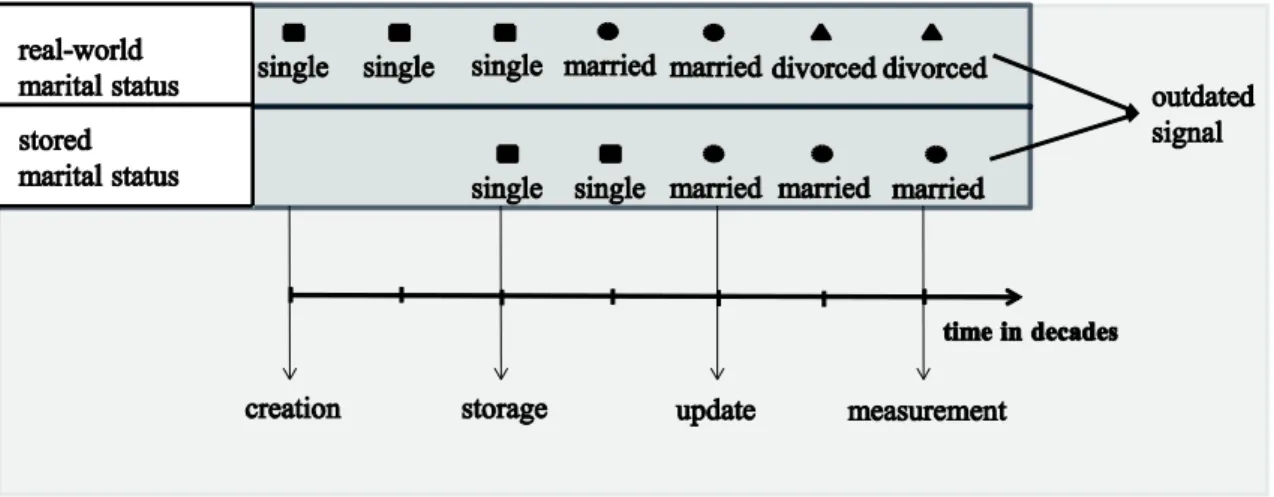
To illustrate this idea consider Figure 1, where the change of marital status information over time is exemplified. At the time of storage (three decades after
Figure 1. Illustration of the temporal change of real-world information.
creation) the stored and the real-world marital status coincide and both are single. Thus, the information is up to date. However, one decade after storage the person gets married and the two values do not coincide anymore. One more decade later the information is updated, so the stored and the real-world marital status coincide again and are both married. Then, after one additional decade, the person gets divorced. As a result, at the time of measurement the stored marital status is married, while the real-world marital status is divorced.
In this case, existing metrics for currency may deliver a low metric value for the correspondence between the stored and the real-world marital status at the time of measurement. Thus, the decision-maker will probably decide not to use the stored information at all to avoid wrong decisions. As a result, the stored information becomes worthless. However, if at the time of measurement, in addition to the low metric value,
9 the decision-maker also knows the distribution of the real-world marital status, based on the stored marital status in the previous periods (e.g. married with a probability of 0.2 and divorced with a probability of 0.8), then the decision can be adjusted
correspondingly. Thus, even though the stored information is outdated, it may still be used to support decisions and is not worthless anymore.
In order to determine the distribution of the real-world information at the time of measurement, we model its temporal change as a stochastic process. A stochastic
process {𝑌𝑡, 𝑡 ∈ 𝑇} is defined over the probability space (Ω, ℱ, 𝑃) with the parameter set 𝑇, often interpreted as time. For a given 𝑡 ∈ 𝑇, the function 𝜔 → 𝑌𝑡(𝜔), Ω → 𝐼 is a random variable defined over (Ω, ℱ, 𝑃) with a range 𝐼, which can be discrete or
continuous. Let {𝑌𝑡, 𝑡 ∈ 𝑇} be the stochastic process describing the temporal change of real-world information, where the values3 𝑦𝑡 ∈ 𝐼 of the random variables 𝑌𝑡 are called signals and the range 𝐼 is called information space. Then 𝑌0 denotes the random variable describing real-world information (e.g. income, address, marital status) at the time of creation 𝑡 = 0, where it is given by the signal 𝑦0 ∈ 𝐼 (e.g. single). Real-world
information changes over time according to the definition of {𝑌𝑡, 𝑡 ∈ 𝑇}, and at the time of storage/update 𝑡 = 𝑡0 ≥ 04 takes the value 𝑌𝑡0 = 𝑦𝑡0 (e.g. married). Finally, at the time of measurement 𝑡 = 𝑡0+ 𝑝, 𝑝 ≥ 0 periods after storage, real-world information is distributed according to the random variable 𝑌𝑡0+𝑝 and the signal 𝑦𝑡0+𝑝 is not known to
3 These values differ from the normative concept of the value of information addressed later.
4 The parameter 𝑡0 denotes the time of storage if no update took place and the time of update otherwise. For simplicity, from now on we will only use storage when referring to it, but will mean both.
10 the decision-maker. The distribution of 𝑌𝑡0+𝑝 is exactly the indication about the real- world information, which can be used by the decision-maker to support the decision.
In the following, we present two extended metrics to determine the distribution of 𝑌𝑡0+𝑝. These are the general form of the extended metric referring to currency and the Markov form of the extended metric referring to currency. If all the real-world signals before the time of measurement are known (i.e. 𝑦0, 𝑦1,…, 𝑦𝑡0+𝑝−1), then the
distribution of 𝑌𝑡0+𝑝 can be determined very precisely. This is the general form of the extended metric referring to currency. In the above marital status example, this implies that the real-world signals in the periods between creation (i.e. single) and storage (i.e.
divorced) are known.
However, in many realistic situations neither the real-world signals before storage, nor the ones after that are known to the decision-maker. Thus, we also
determine the distribution of 𝑌𝑡0+𝑝, based only on the stored signal 𝑦𝑡0 (i.e. married in the above example), by making an additional assumption regarding the stochastic process. This is the Markov form of the extended metric referring to currency, which is not as precise as the general form, but more appropriate for some practical applications.
We begin with the general form of the extended metric referring to currency.
The general form of the extended metric referring to currency is defined for 𝑝 ≥ 0, 𝑡0 ≥ 0 as:
𝑚𝑔(𝑦𝑡0+𝑝|𝑦𝑡0+𝑝−1, 𝑦𝑡0+𝑝−2, … , 𝑦𝑡0, … , 𝑦0, 𝑝, 𝑡0) ≔
𝑓𝑌𝑡0+𝑝|𝑌𝑡0+𝑝−1,𝑌𝑡0+𝑝−2,…,𝑌𝑡0,…,𝑌0(𝑦𝑡0+𝑝|𝑦𝑡0+𝑝−1, 𝑦𝑡0+𝑝−2, … , 𝑦𝑡0, … , 𝑦0), 𝑦𝑖 ∈ 𝐼 ∀𝑖 ≥ 0 (1)
where {𝑌𝑡, 𝑡 ∈ 𝑇} is the general stochastic process describing the temporal change of real-world information, 𝑡0 ≥ 0 is the time of storage and 𝑝 ≥ 0 represents the number of periods between storing the information and measuring currency.
11 𝑓𝑌𝑡0+𝑝|𝑌𝑡0+𝑝−1,𝑌𝑡0+𝑝−2,…,𝑌𝑡0,…,𝑌0(𝑦𝑡0+𝑝|𝑦𝑡0+𝑝−1, 𝑦𝑡0+𝑝−2, … 𝑦𝑡0, … , 𝑦0), 𝑦𝑖 ∈ 𝐼 ∀𝑖 ≥ 0 is the conditional probability density (mass) function at the real-world signal 𝑦𝑡0+𝑝 for the time of measurement 𝑡0+ 𝑝, provided that the real-world signals in the periods before the measurement were 𝑦𝑡0+𝑝−1, 𝑦𝑡0+𝑝−2, … , 𝑦𝑡0, … , 𝑦0. In addition,
𝑚𝑔(𝑦𝑡0+𝑝|𝑦𝑡0+𝑝−1, 𝑦𝑡0+𝑝−2, … , 𝑦𝑡0, … , 𝑦0, 𝑝, 𝑡0), 𝑦𝑡0+𝑝 ∈ 𝐼 ∀𝑖 ≥ 0 is the corresponding metric, which does not result in a single value, but rather a distribution over the possible signals 𝑦𝑡0+𝑝 conditioned on the given real-world signals
𝑦𝑡0+𝑝−1, 𝑦𝑡0+𝑝−2, … , 𝑦𝑡0, … , 𝑦0.
In the case of discrete information space, the general form of the extended metric gives the probabilities for the possible real-world signals at the time of measurement, conditioned on the given real-world signals in the periods before the measurement. In contrast, the metric for currency by Heinrich and Klier (2015) gives the probability that the real-world information did not change between the time of storage 𝑡0 and the time of measurement 𝑡0+ 𝑝 (i.e. the probability that the stored signal is still up to date). Thus, the contribution of our metric is that it also provides the
probabilities for the possible real-world signals at the time of measurement which differ from than the stored one. This is important especially in the case when the
correspondence between the stored signal and its real-world counterpart is indicated to be low, because then the decision-maker can adjust his/her decision, based on the probabilities of the general form of the extended metric.
The real-world signals 𝑦𝑡0+𝑝−1, 𝑦𝑡0+𝑝−2, … , 𝑦𝑡0, … , 𝑦0 before the time of measurement are required as input parameters for the general form of the extended metric. However, as mentioned above, in several realistic situations, only 𝑦𝑡0 is known to the decision-maker (i.e. neither the history before storage nor the change of
12 information after storage is known). This is similar to the problem described by
Heinrich, Klier, and Görz (2012) and Heinrich and Klier (2015), that the time of
creation of a signal is often not known. To address this problem, similarly to Heinrich et al. (2012), we consider the time of storage and not the time of creation in determining currency, and restrict the above general stochastic process {𝑌𝑡, 𝑡 ∈ 𝑇} to a process which possesses the Markov property (Nelson, 1995; Wechsler & Even, 2012). Thus
𝑓𝑌𝑡0+𝑖+1|𝑌𝑡0+𝑖,𝑌𝑡0+𝑖−1,𝑌𝑡0+𝑖−2,…,𝑌0(𝑦𝑡0+𝑖+1|𝑦𝑡0+𝑖, 𝑦𝑡0+𝑖−1, 𝑦𝑡0+𝑖−2, … , 𝑦0) =
𝑓𝑌𝑡0+𝑖+1|𝑌𝑡0+𝑖(𝑦𝑡0+𝑖+1|𝑦𝑡0+𝑖), ∀𝑖 ∈ [0, 𝑝 − 1] (2)
This property implies for 𝑖 = 0 that the change of the real-world information one period after storage depends only on the real-world signal at the time of storage and not on its history before storage. As a result, the signals 𝑦𝑡0−1, 𝑦𝑡0−2, … , 𝑦0 are not required as inputs anymore. Moreover, by recursively applying Equation (2), we can easily derive the distribution of real-world information at the time of measurement without knowing the real-world signals 𝑦𝑡0+𝑝−1, 𝑦𝑡0+𝑝−2, … , 𝑦𝑡0+1 in the periods between storage and measurement. If the time of measurement is 𝑝 = 2 periods after storage, then due to Equation (2) the distribution of real-world information 𝑌𝑡0+2 depends on 𝑓𝑌𝑡0+2|𝑌𝑡0+1 and the real-world signal at 𝑡0 + 1, which is unknown to the decision-maker. However, again due to the Markov property, the distribution of the real-world information 𝑌𝑡0+1 can be derived from 𝑓𝑌𝑡0+1|𝑌𝑡0 and the stored signal 𝑦𝑡0 which is known to the decision-maker. This recursive idea can analogously be applied for 𝑝 > 2 to estimate 𝑓𝑌𝑡0+𝑝|𝑌𝑡0(𝑦𝑡0+𝑝|𝑦𝑡0).
We define the Markov form of the extended metric referring to currency for 𝑝 >
0, 𝑡0 ≥ 0 as:
13 𝑚𝑚(𝑦𝑡0+𝑝|𝑦𝑡0, 𝑝, 𝑡0) ≔ 𝑓𝑌𝑡0+𝑝|𝑌𝑡0(𝑦𝑡0+𝑝|𝑦𝑡0), 𝑦𝑡0+𝑝, 𝑦𝑡0 ∈ 𝐼 (3)
where {𝑌𝑡, 𝑡 ∈ 𝑇} is a stochastic process which possesses the Markov property
and 𝑚𝑚(𝑦𝑡0+𝑝|𝑦𝑡0, 𝑝, 𝑡0), 𝑦𝑡0+𝑝 ∈ 𝐼 is the corresponding metric, which does not result in a single value, but rather a distribution over the possible signals 𝑦𝑡0+𝑝 conditioned on the given stored signal 𝑦𝑡0. The conditional probability density (mass) function of the real-world information 𝑌𝑡0+𝑝 at the time of measurement 𝑡0+ 𝑝 provided that the stored signal is 𝑌𝑡0 = 𝑦𝑡0 (i.e. 𝑓𝑌𝑡0+𝑝|𝑌𝑡0(𝑦𝑡0+𝑝|𝑦𝑡0)) is derived recursively as discussed above.
In the following two subsections, we illustrate how the Markov form of the extended metric referring to currency can be applied to two scenarios: information with discrete information space such as marital status or address information, and
information with continuous information space such as income information. The application of the general form of the extended metric referring to currency can be illustrated in a similar fashion.
2.1. Discrete information space scenario
In this subsection, we consider a scenario where the information space consists of a finite number of values. This implies that after storing the signal at 𝑡0 the real-world signal one period after storage can either change to finitely many other values or stay the same. For example, if the marital status of a person is stored as single, then one period after storage the real-world marital status can take only one of the values {single, married, divorced, widowed}. The same holds for address information, where the number of possible addresses a person could move to one period after storage is high, but still finite. As a result, for any stored signal and each possible value in the
information space, the probability that the real-world information takes this value one
14 period after storage can be determined based on publicly available statistical data or other data sources. For example, for the stored single marital status, the probabilities that the person got married, divorced, widowed or stayed single one period after storage are determined from the marriage, divorce and mortality rates in a certain country (e.g.
from the German Federal Bureau of Statistics in Germany). The same holds for address information, where for each possible address the probability that a person moved to it (or remained there) one period after storage is determined from the residential mobility rates within the same street, district, city, province or country (e.g. also based on data from the German Federal Bureau of Statistics). These probabilities, called transition probabilities, can be determined in a similar fashion for any two consecutive periods after storage.
After their determination, transition probabilities are used to obtain the value of the Markov form of the extended metric as follows: let the process {𝑌𝑡, 𝑡 ∈ 𝑇} be a Markov chain5 with an information space 𝐼 = {𝑦1, … , 𝑦𝑛}, 𝑛 ≥ 1 consisting of mutually exclusive signals. Then 𝑚𝑚(𝑦𝑗|𝑦𝑘, 1, 𝑡0), 𝑗, 𝑘 ∈ [1, . . , 𝑛], as defined in Equation (3), is the transition probability from a stored signal 𝑦𝑘 at the time of storage 𝑡0 to a real-world signal 𝑦𝑗 one period after storage. Similarly, 𝑚𝑚(𝑦𝑗|𝑦𝑠, 1, 𝑡0+ (𝑝 − 1)), 𝑝 > 0 is the transition probability from a stored signal 𝑦𝑠 to a real-world signal 𝑦𝑗 between any two consecutive periods after storage. To calculate the values of the extended metric
𝑚𝑚(𝑦𝑗|𝑦𝑘, 𝑝, 𝑡0) ∀𝑗, ∀𝑘 ∈ {1, … , 𝑛}, 𝑡0 ≥ 0, 𝑝 > 0, we use the above transition probabilities as inputs to the following recursive model, which is based on the law of total probability:
5 Note that a metric for accuracy, based on Markov chains, is presented in Wechsler and Even (2012).
15
𝑝 = 1: 𝑚𝑚(𝑦𝑗|𝑦𝑘, 1, 𝑡0) is determined as described above;
𝑝 > 1: 𝑚𝑚(𝑦𝑗|𝑦𝑠, 1, 𝑡0+ (𝑝 − 1)) is determined as described above and 𝑚𝑚(𝑦𝑗|𝑦𝑘, 𝑝, 𝑡0) = ∑𝑛𝑠=1𝑚𝑚(𝑦𝑗|𝑦𝑠, 1, 𝑡0+ (𝑝 − 1))𝑚𝑚(𝑦𝑠|𝑦𝑘, 𝑝 − 1, 𝑡0)
The result from the application of the extended metric is a distribution over the possible real-world signals at the time of measurement, conditioned on the stored signal.
This implies that the decision-maker can adjust the decision, if the probability that the stored signal corresponds to the real-world signal is low. For example, if the stored signal is the marital status single and it is now indicated that the person is married with high probability at the time of measurement, then the decision should correspond rather to a married marital status than to a single one (cf. section 4). The same holds for stored address information. If according to the extended metric a person with a given stored address should with high probability have moved to another city, then the new city should be considered in the decision.
We can easily extend the above approach to apply it to a multidimensional information space by using multivariate Markov chains. This is very useful for example in sales campaigns, because often more than one attribute of the customer influences the demand (e.g. gender, education and marital status) and the temporal change of these attributes over time are not independent of each other.
2.2. Continuous information space scenario
In this subsection we consider a scenario where the information space consists of an infinite number of values. This implies that after storing the signal at 𝑡0 the real-world signal one period after storage can either change to infinitely many other values or stay the same. For example, if the stored signal is the income of a person, then the real-world
16 income one decade after storage can take any non-negative value. As opposed to the previous subsection, in this case for each stored signal it is necessary to determine a continuous (transition) probability distribution over the possible real-world signals in the next period. For example, if the stored signal is the income of a given person, then the distribution of the logarithm of the real-world income one period after storage will be normal with expected value depending on the logarithm of the stored income (Guvenen, 2009; Hryshko, 2009). A similar approach is then applied to any two consecutive periods after storage. In order to derive this distribution, historical
information is used such as income information of customers or publicly available panel data (SOEP, 2012, cf. section 4).
To determine the value of the Markov form of the extended metric, we thus model the process {𝑌𝑡, 𝑡 ∈ 𝑇} as an autoregressive process of order one (Brooks, 2008).
This implies that for a measurement made one period after storage (i.e. 𝑝 = 1):
𝑌𝑡0+1= 𝜇 + 𝜙𝑌𝑡0+ ε𝑡0 (4)
where {ε𝑡, 𝑡 ∈ 𝑇} is a white noise process with variance 𝜎2 and 𝜇, 𝜙 are scalars. Thus, the extended metric is the conditional density function of a normally distributed random variable:
𝑚𝑚(𝑦𝑡0+1|𝑦𝑡0, 1, 𝑡0) = 1
√2𝜋𝜎2𝑒−(𝑦𝑡0+1−( 𝜇+𝜙𝑦𝑡0))2
2𝜎2 (5)
Currency one period after storage can be interpreted as the value of the above density function at 𝑦𝑡0 (i.e. 𝑚𝑚(𝑦𝑡0|𝑦𝑡0, 1, 𝑡0)). However, as opposed to the previous subsection, since we have a continuous information space here, 𝑚𝑚(𝑦𝑡0|𝑦𝑡0, 1, 𝑡0)
17 cannot be interpreted as probability. In addition, the normal distribution assumption can be easily relaxed by modifying 𝜇, 𝜙, and {ε𝑡, 𝑡 ∈ 𝑇}.
Based on Equation (4), for 𝑝 = 2 the following holds:
𝑌𝑡0+2= 𝜇 + 𝜙𝑌𝑡0+1+ ε𝑡0+1= (1 + 𝜙)𝜇 + 𝜙2𝑌𝑡0 + 𝜙ε𝑡0 + ε𝑡0+1 (6)
which implies that
𝑚𝑚(𝑦𝑡0+2 |𝑦𝑡0, 2, 𝑡0) = 1
√2𝜋𝜎2(1+𝜙2)𝑒−
(𝑦𝑡0+2− ((1+𝜙)𝜇+𝜙2𝑦𝑡0))2
2𝜎2(1+𝜙2) (7)
The extended metric for 𝑝 > 2 is analogously estimated:
𝑚𝑚(𝑦𝑡0+𝑝 |𝑦𝑡0, 𝑝, 𝑡0) = 1
√2𝜋𝜎21−𝜙2𝑝 1−𝜙2
𝑒
−(𝑦𝑡0+𝑝− (𝜇
1−𝜙𝑝1−𝜙 +𝜙𝑝𝑦𝑡0))2 2𝜎2(1−𝜙2𝑝
1−𝜙2)
(8)
Therefore, upon measurement the decision-maker knows that the distribution of the real-world signal conditioned on the stored signal is normal with the corresponding expected value and variance and can consider this distribution in the decision. In the example with income, this implies that the distribution of the logarithm of the real- world income at the time of measurement is normal with expected value depending on the logarithm of the stored income, where the parameters of the autoregressive process can be estimated by means of historical data (cf. section 4).
In this section, we presented an extended metric referring to currency and applied it to two scenarios with a discrete and a continuous information space,
respectively. In the next section, we present our approach for incorporating this metric in decision-making under uncertainty.
18 3. Modelling the influence of currency on decision-making under
uncertainty
3.1. Development of the model
In this subsection, we model the influence of currency on decision-making under uncertainty by extending the normative concept of the value of information. Thus, we first present this concept. The normative concept of the value of information (𝑉𝑜𝐼) is defined as6:
𝑉𝑜𝐼: = ∫ 𝑚𝑎𝑥𝑦∈𝐼 𝑥∈𝑋∫𝑠∈𝐶𝑤(𝑥, 𝑠)𝑓𝑆|𝑌(𝑠|𝑦)𝑑𝑠𝑓𝑌(𝑦)𝑑𝑦 − 𝑚𝑎𝑥𝑥∈𝑋∫𝑠∈𝐶𝑤(𝑥, 𝑠)𝑓𝑆(𝑠)𝑑𝑠 (9)
where
𝑆 is the random variable describing the states of nature with range (state space) 𝐶;
𝑌 is the random variable describing the signals with range (information space) 𝐼;
𝑓𝑆|𝑌 denotes the conditional density function of the states of nature for a particular signal;
𝑓𝑌 represents the density function of the signals;
𝑓𝑆 stands for the density function of the states of nature;
𝑋 expresses the set of possible choices of the decision-maker;
𝑤(𝑥, 𝑠) is the payoff function for a given choice-state (𝑥, 𝑠) combination.
The idea is that the decision-maker has to make an ex ante decision in an uncertain environment without knowing the state of nature that will occur in the future
6 cf. Hilton(1981) and Lawrence(1999), where up to date information is implicitly assumed.
19 (i.e. after the instant of the decision). Without additional information, the expected payoff would depend only on the distribution of the states of nature 𝑓𝑆 and is exactly the value in the second term of Equation (9; i.e. the subtrahend).
The uncertainty in the environment, which we shall call environmental uncertainty from now on, can be reduced by obtaining additional information that indicates which state of nature will occur in the future. This information is represented by the random variable 𝑌, values of which are the signals as discussed in the previous section. If a signal 𝑦 ∈ 𝐼 indicates with certainty which state of nature will occur, it eliminates environmental uncertainty completely. However, a signal 𝑦 can also deliver a ‘noisy’ indication. This means that it does not indicate one particular state of nature with certainty, but a number of states with their corresponding probabilities
(e.g. ∃𝑠1, ∃𝑠2 ∈ 𝐶, 𝑠1 ≠ 𝑠2 with 𝑓𝑆|𝑌(𝑠1|𝑦) > 0 and 𝑓𝑆|𝑌(𝑠2|𝑦) > 0). Then, the signal still reduces environmental uncertainty, but does not eliminate it completely. Based on the signal, the decision-maker may change the decision so that it leads to a higher expected payoff. Thus, 𝑉𝑜𝐼 is calculated as the difference between the expected optimal payoff when additional information is considered and the expected optimal payoff without considering it. Note that for simplicity the definition in Equation (9) assumes that the decision-maker is risk neutral. This is realistic when companies aim only at maximizing their expected profit. However, the model can be easily adjusted for a risk- averse or a risk-seeking decision-maker.
The formula in Equation (9) assumes that the signal corresponds to the real- world one at the time of the decision. However, in many realistic situations this is not the case, as the (stored) signal can be outdated (cf. section 2), and thus the
correspondence with the real-world signal is indicated as less than perfect. Then the decision-maker faces another kind of uncertainty in addition to the environmental
20 uncertainty, which we call quality uncertainty. Quality uncertainty should be taken into account since it can lead to a change in the ex ante decision and, as a result, to higher ex post value.
We thus extend 𝑉𝑜𝐼 by explicitly incorporating quality uncertainty in the form of our extended metric referring to currency. For illustration purposes, we use the Markov form of the extended metric (i.e. Equation 3), but the model can be analogously applied to the general form of the metric (i.e. Equation 1).
In Equation (10) we present our model, where 𝑉𝑜𝐼 after considering quality uncertainty (𝑉𝑜𝐼𝑄) depends on the time of storage 𝑡0 ≥ 0, and on the number of periods 𝑝 between storage and using the information to support decision-making (i.e.
the time of measurement). Moreover, in Equation (11) we define the value of a signal (𝑉𝑜𝑆) 𝑦𝑡0 stored at time 𝑡0. The reason for this second definition is that a decision is taken based on the observed signal 𝑦𝑡0 stored at time 𝑡0 and decisions may differ for different signals resulting in different expected payoffs.
𝑉𝑜𝐼𝑄(𝑡0, 𝑝) ≔
∫ 𝑚𝑎𝑥𝑥∈𝑋∫𝑦 ∫𝑠∈𝐶𝑤(𝑥, 𝑠)𝑓𝑆|𝑌𝑡0+𝑝(𝑠|𝑦𝑡0+𝑝)𝑑𝑠𝑚𝑚(𝑦𝑡0+𝑝 |𝑦𝑡0, 𝑝, 𝑡0)𝑑𝑦𝑡0+𝑝𝑓𝑌𝑡0(𝑦𝑡0)𝑑𝑦𝑡0
𝑡0+𝑝∈𝐼
𝑦𝑡0∈𝐼
−𝑚𝑎𝑥𝑥∈𝑋∫𝑠∈𝐶𝑤(𝑥, 𝑠)𝑓𝑆(𝑠)𝑑𝑠 (10)
𝑉𝑜𝑆(𝑦𝑡0, 𝑡0, 𝑝) ≔
𝑚𝑎𝑥𝑥∈𝑋∫𝑦 ∫𝑠∈𝐶𝑤(𝑥, 𝑠)𝑓𝑆|𝑌𝑡0+𝑝(𝑠|𝑦𝑡0+𝑝)𝑑𝑠𝑚𝑚(𝑦𝑡0+𝑝 |𝑦𝑡0, 𝑝, 𝑡0)𝑑𝑦𝑡0+𝑝
𝑡0+𝑝∈𝐼 (11)
The main idea behind Equation (10) is that at 𝑡0+ 𝑝, the decision-maker observes only the stored signal 𝑦𝑡0 and must make a decision based on it (for the general form of the extended metric 𝑦𝑡0+𝑝−1, 𝑦𝑡0+𝑝−2, … , 𝑦𝑡0+1, 𝑦𝑡0−1, … , 𝑦0 are additionally taken into account). If the stored signal is indicated to be perfectly up to
21 date (i.e. the corresponding probability in the discrete case is 1), it coincides with the real-world signal and quality uncertainty is completely eliminated. However, if the stored signal is indicated not to be perfectly up to date (i.e. the corresponding probability in the discrete case is smaller than 1), then it delivers only a ‘noisy’
indication about the real-world signal 𝑦𝑡0+𝑝 at 𝑡0+ 𝑝 and quality uncertainty exists represented by the Markov form of the extended metric 𝑚𝑚(𝑦𝑡0+𝑝 |𝑦𝑡0, 𝑝, 𝑡0). The function 𝑓𝑆|𝑌𝑡0+𝑝 represents environmental uncertainty as discussed above.
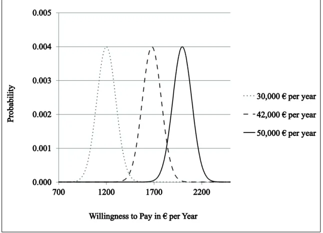
To illustrate the idea, consider the income example from above. The signal 𝑦𝑡0 represents the income of the customer at the time of the storage (e.g. one decade ago).
The signal 𝑦𝑡0+𝑝 represents the income of the customer at the time of the decision. The function 𝑚𝑚(𝑦𝑡0+𝑝 |𝑦𝑡0, 𝑝, 𝑡0) represents the quality uncertainty about the real-world income, and 𝑓𝑆|𝑌𝑡0+𝑝 represents the environmental uncertainty regarding the willingness to pay of the customers (i.e. customers with the same income would not necessarily have the same willingness to pay; cf. section 4). Thus, as mentioned above, quality uncertainty and environmental uncertainty are two different kinds of uncertainty and should both be taken into account by the decision-maker to avoid wrong decisions.
The contribution of our model as opposed to Equation (9) is that for a given stored signal, the choice in the first term of 𝑉𝑜𝐼𝑄 may be adapted when considering quality uncertainty and will possibly differ from the choice in the first term of 𝑉𝑜𝐼 (which considers only environmental uncertainty), leading to different payoffs. In the next subsection we derive the conditions under which this happens.
22 3.2. Conditions for a change in the optimal decision when considering
currency
As mentioned above, information is valuable because it may result in a different indication about the future states of nature and thus in a change of the decision. The same holds for currency. If after considering it, the indication about future states of nature changes, then so may the decision. In Theorem 1 we provide the conditions under which this happens. The proof of Theorem 1 is provided in the Appendix.
Theorem 1: Let 𝑥𝑤𝑜(𝑦𝑡0, 𝑡0, 𝑝) be the optimal choice of the decision-maker at (𝑡0+ 𝑝) for a signal 𝑦𝑡0stored at 𝑡0 without considering currency (cf. Equation 9) and let 𝑥𝑤(𝑦𝑡0, 𝑡0, 𝑝) be the optimal choice of the decision-maker at (𝑡0+ 𝑝) for the same stored signal when considering currency (cf. Equation 10). Here we assume that
𝜕2𝑤(x,𝑠)
𝜕2𝑥 < 0 ∀𝑥 ∈ 𝑋, ∀𝑠 ∈ 𝐶 (i.e. the payoff function is concave in the choice of the decision-maker).
Let, in addition,
𝑔(𝑠, 𝑦𝑡0, 𝑝): = ∫𝑦 𝑓𝑆|𝑌𝑡0+𝑝(𝑠|𝑦𝑡0+𝑝)𝑚𝑚(𝑦𝑡0+𝑝 |𝑦𝑡0, 𝑝, 𝑡0)𝑑𝑦𝑡0+𝑝
𝑡0+𝑝∈𝐼 (12)
𝒮0(𝑦𝑡0): = {𝑠 ∈ 𝐶: 𝑔(𝑠, 𝑦𝑡0, 𝑝) = 𝑓𝑆|𝑌𝑡0+𝑝(𝑠|𝑦𝑡0)} (13)
Then
(1) 𝑥𝑤𝑜(𝑦𝑡0, 𝑡0, 𝑝) = 𝑥𝑤(𝑦𝑡0, 𝑡0, 𝑝), if 𝒮0(𝑦𝑡0) = 𝐶 (2) 𝑥𝑤𝑜(𝑦𝑡0, 𝑡0, 𝑝) < 𝑥𝑤(𝑦𝑡0, 𝑡0, 𝑝), if
∫𝑠∈𝐶𝜕𝑤(𝑥𝑤𝑜(𝑦𝜕𝑥𝑡0,𝑡0,𝑝) ,𝑠)(𝑔(𝑠, 𝑦𝑡0, 𝑝) − 𝑓𝑆|𝑌𝑡0+𝑝(𝑠|𝑦𝑡0)) 𝑑𝑠 > 0 (14)
23 (3) 𝑥𝑤𝑜(𝑦𝑡0, 𝑡0, 𝑝) > 𝑥𝑤(𝑦𝑡0, 𝑡0, 𝑝), if
∫𝑠∈𝐶𝜕𝑤(𝑥𝑤𝑜(𝑦𝜕𝑥𝑡0,𝑡0,𝑝) ,𝑠)(𝑔(𝑠, 𝑦𝑡0, 𝑝) − 𝑓𝑆|𝑌𝑡0+𝑝(𝑠|𝑦𝑡0)) 𝑑𝑠 < 0 (15)
To discuss Theorem 1, let us first consider the interpretation of the function 𝑔(𝑠, 𝑦𝑡0, 𝑝). Since ∫𝑠∈𝐶𝑔(𝑠, 𝑦𝑡0, 𝑝)𝑑𝑠 = 1, this function can be interpreted as the distribution of the states of nature, based on the stored signal 𝑦𝑡0 after considering both environmental and quality uncertainty. Thus the set 𝒮0(𝑦𝑡0) consists of all the states, where the probability of occurrence (for a discrete state space) when considering currency coincides with the probability of occurrence without considering currency. If this is the case for all possible states, then the level of uncertainty (after considering both environmental and quality uncertainty) stays the same as with only environmental uncertainty, and naturally the choice does not change. This is the interpretation behind (1). In contrast, (2) and (3) state that the solution changes when the probability of occurrence of some states when considering currency changes as opposed to that without considering currency. For example, if a state of nature is much more probable when considering currency and an increase in 𝑥𝑤(𝑦𝑡0, 𝑡0, 𝑝) increases the payoff in this state, then 𝑥𝑤(𝑦𝑡0, 𝑡0, 𝑝) may be higher than 𝑥𝑤𝑜(𝑦𝑡0, 𝑡0, 𝑝).
To illustrate this point, consider again the income example from above. In the case where we consider currency and the real-world income is indicated to be the same as the stored one (and environmental uncertainty stays the same), the offer will not change. If the stored income indicates higher real-world income (and environmental uncertainty stays the same), then the customer will receive a more expensive offer. If, on the contrary, it indicates lower real-world income (and environmental uncertainty stays the same), s/he will receive a cheaper offer. The change in the decision in the last
24 two cases can lead to a change in the relationship between currency and the value of a signal, as discussed in the next subsection.
3.3. The role of the model in the TDQM methodology
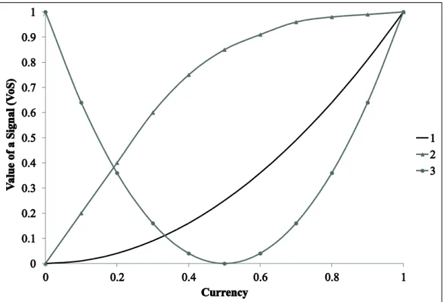
In this subsection, we discuss the role of our model in the third phase of the TDQM methodology. In particular, in Figure 2 we illustrate three possible dependencies between 𝑉𝑜𝑆 (i.e. Equation 11) and the level of currency of the stored signal. For illustration purposes, we concentrate in the following on the currency of the stored signal, which represents one of the most important values of the extended metric
referring to currency for a discrete information space (cf. section 2). Note, however, that a similar analysis can be done with any other value of the extended metric referring to currency.
Curve 1 implies that 𝑉𝑜𝑆 is a convex increasing function of currency (i.e. it increases at an increasing rate). This dependency occurs when the decision situation requires a stored signal with a (very) high metric value for a reliable decision (i.e. the indicated correspondence between the stored and the real-world signal must be high).
An example for such a case is the stock price for an investor who needs to decide where to invest. There, it is extremely important that the stock price is as up to date as
possible.
Similarly, Curve 2 implies that 𝑉𝑜𝑆 is a concave increasing function of currency and thus increases with currency at a decreasing rate. This dependency occurs when it is important for the decision-maker that the stored information is not too outdated, but it must not necessarily be perfectly up to date for a reliable decision. An example for such a case is the income information for a sales campaign, as discussed above. It is
25 important that the stored income corresponds to some degree to the real-world one, but this correspondence does not have to be perfect for a successful offer.
Figure 2. Value of a Signal (VoS) as a function of currency.
In both Curves 1 and 2 𝑉𝑜𝑆 is an increasing function of currency, which may support the assumption made by many authors (cf. section 1). As a result, a stored signal with higher currency should also have a higher 𝑉𝑜𝑆. However, there is another possible relationship (i.e. Curve 3), which exists in applications but is not considered in the literature. Curve 3 suggests that a stored signal with lower currency may also be valuable, because the decision-maker may learn from the knowledge about the low currency of the stored signal and adjust the decision accordingly. To illustrate this idea, consider a discrete information space consisting of only two signals (i.e. 𝐼 = {𝑦, 𝑦′}).
Let the stored signal be 𝑦 and the currency of this signal be 𝑞 (i.e. 𝑚𝑚(𝑦 |𝑦, 𝑝, 𝑡0) = 𝑞).
This implies that 𝑚𝑚(𝑦′ |𝑦, 𝑝, 𝑡0) = 1 − 𝑞 meaning that the probability that the real-
26 world signal is 𝑦′ is (1 − 𝑞). Therefore, if the stored signal is very outdated (i.e. 𝑞 is very low), then (1 − 𝑞) is very high and the decision-maker knows almost with
certainty that the real-world signal is 𝑦′, despite the low quality of the stored signal. As a result, s/he can adjust the decision correspondingly, and the value of the stored signal increases. In order to determine this decision, the decision-maker first needs to find the optimal solutions in Equation (10). In the next subsection, we discuss possible
approaches for doing this, based on the field of stochastic programming.
3.4. Solution approaches
Our approach for considering currency in decision-making is described by Equation (10), where two optimal choices need to be determined. On the one hand, we need to determine the optimal choice based on the stored signal, by considering both quality and environmental uncertainty (i.e. the first term in Equation 10). On the other hand, the optimal choice based only on the stored signal and environmental uncertainty is required. For both of these cases, in the following, we present possible solution
approaches from the field of stochastic programming. Specifically, Equation (10) can be rewritten as:
𝑉𝑜𝐼𝑄(𝑡0, 𝑝) ≔ 𝐸𝑌𝑡0(𝑚𝑎𝑥𝑥∈𝑋𝐸𝑌𝑡0+𝑝|𝑌𝑡0(𝐸𝑆|𝑌𝑡0+𝑝(𝑤(𝑥, 𝑆)))) − 𝑚𝑎𝑥𝑥∈𝑋𝐸𝑆(𝑤(𝑥, 𝑆)) (16)
where 𝐸𝑌𝑡0+𝑝|𝑌𝑡0 is the conditional expectation with respect to the random variable 𝑌𝑡0+𝑝, modelling the real-world information; 𝐸𝑌𝑡0 is the expectation with respect to 𝑌𝑡0
standing for the stored information; 𝐸𝑆 is the expectation with respect to the states of nature; and 𝐸𝑆|𝑌𝑡0+𝑝 is the conditional expectation of the states of nature on the real- world information. The terms 𝑚𝑎𝑥𝑥∈𝑋𝐸𝑌𝑡0+𝑝|𝑌𝑡0(𝐸𝑆|𝑌𝑡0+𝑝(𝑤(𝑥, 𝑆))) and
27 𝑚𝑎𝑥𝑥∈𝑋𝐸𝑆(𝑤(𝑥, 𝑆)) are representative for (unconstrained) stochastic programming problems (Birge & Louveaux, 2011; Gentle, Härdle, & Mori, 2012; Shapiro &
Dentcheva, 2014). If these terms can be characterised by a closed-form function of 𝑥, then finding a solution would be equivalent to solving an unconstraint (non-)linear optimisation problem, for which there are different approaches in the literature (Hillier
& Lieberman, 2004). However, usually this is not the case and other approaches from the field of stochastic programming must be applied.
In the case that no closed-form representation is available and for continuous random variables, the integrals in Equation (16) can be approximated with numerical integration procedures (Birge & Louveaux, 2011) such as quadrature rules for the term 𝑚𝑎𝑥𝑥∈𝑋𝐸𝑆(𝑤(𝑥, 𝑆)) and Monte Carlo methods for
𝑚𝑎𝑥𝑥∈𝑋𝐸𝑌𝑡0+𝑝|𝑌𝑡0(𝐸𝑆|𝑌𝑡0+𝑝(𝑤(𝑥, 𝑆))) (Robert & Casella, 2010). Another possibility would be to apply stochastic approximation. The basic idea is to stochastically explore 𝑋 and thus determine the maximum of the objective function. Examples for such approaches are stochastic gradient search and simulated annealing (Gentle et al., 2012;
Robert & Casella, 2010). Finally, genetic algorithms, which are based on ideas from natural evolution developments, can also be applied. As opposed to stochastic approximation, genetic algorithms explore 𝑋 by simultaneously considering a set of possible values instead of only one value (Gentle et al., 2012) and refine this set until the highest fitness is achieved. The presented solution approaches can then be used to determine both optimal choices with and without considering currency and thus 𝑉𝑜𝐼𝑄(𝑡0, 𝑝) in Equation (16). Generally, the selection of the approach depends on the particular mathematical formulation and on the properties of the different functions in Equation (16).This completes the presentation of our approach. In the next section we demonstrate its relevance by applying it to two scenarios from the insurance industry.
28 4. Evaluation
In this section we evaluate the presented approach, discuss and interpret the results, and explicate relevant practical implications. We concentrate on two scenarios from the field of sales management in CRM for insurance companies. In our analysis we represent customer databases with the panel data from the SOEP (2012), which was made available to us by the German Socio-Economic Panel Study (SOEP) at the
German Institute for Economic Research (DIW), Berlin. We chose this application field due to the importance of currency for decision-making there. In particular, when
conducting sales campaigns, most insurance companies rely either on their own customer databases or on publicly available information sources and in both cases outdated information may have negative consequences for the success of the campaign.
4.1. General liability insurance scenario
In the first scenario we consider an insurance company, which possesses information regarding the marital status, year of birth (age) and gender of its customers, that was correctly stored in 1998. Thus, the information space is multidimensional, but only the marital status may become outdated. The company is planning to conduct a campaign (in one of the years after 1998) to attract new customers for its general liability insurance by sending different offers per post depending on the marital status of the customers. The company’s decision space thus consists of sending one of four offers (i.e. for single, married, divorced or widowed customers) or not sending an offer at all.
The customer can either accept or reject the corresponding offer. An offer can be
rejected because the customer would not like any general liability insurance. The payoff function is the net profit per person and is calculated based on the annual reports of a number of major insurance companies in Germany as well as on the corresponding
29 postal and labour costs.
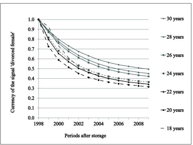
In order to demonstrate the relevance of our metric, for a given age and gender of the customers, we first measure the currency of the marital status information.
Currency is estimated following the interpretation by Heinrich and Klier (2015) with publicly available statistical information about the marriage, divorce and mortality rates in Germany for the years 1998-2009 (German Federal Bureau of Statistics). In Figure 3, the results for the signal ‘divorced female’ are presented. For better illustration, we plotted only the currency for selected groups of customers (e.g. age between 18 and 30).
As we can see, the currency of the marital status information decreases over time and it becomes less than 50% in 2009. This implies that in 2009 the probability that the stored signal is still up to date is lower than the probability that it is not. Therefore, the
company may choose not to consider the stored marital status signal at all. However, if the company possesses an indication about the probability that the customer is married or widowed at the time of the campaign, it can adjust the decision and send the
corresponding offer.
To determine this indication we apply the Markov form of the extended metric referring to currency presented in section 2, and in particular the approach in subsection 2.1 because the information space is discrete. Note that a customer who is married, divorced or widowed can never become single again, and a single customer cannot become divorced or widowed one period later. Table 1 presents the results for a female customer, aged between 18 and 30, whose marital status was stored as ‘divorced’ in 1998. The year of the decision is 2009. As we can see, the probability that such a customer got married in the meantime is in all cases higher than the one that she stayed divorced, which should be taken into account by the decision-maker. As the example shows, the extended metric gives the probabilities for all possible real-world