A decade of dimethyl sulfide (DMS), dimethylsulfoniopropionate (DMSP) and dimethyl sulfoxide (DMSO) measurements in the southwestern Baltic Sea

(1)

https://doi.org/10.5194/bg-18-2161-2021

A decade of dimethyl sulfide (DMS), dimethylsulfoniopropionate (DMSP) and dimethyl sulfoxide (DMSO) measurements in the southwestern Baltic Sea

Yanan Zhao, Cathleen Schlundt, Dennis Booge, and Hermann W. Bange

GEOMAR Helmholtz Centre for Ocean Research Kiel, Düsternbrooker Weg 20, 24105 Kiel, Germany Correspondence:Yanan Zhao (yzhao@geomar.de)

Received: 21 November 2020 – Discussion started: 14 December 2020

Revised: 18 February 2021 – Accepted: 19 February 2021 – Published: 25 March 2021

Abstract. Dimethyl sulfide (DMS), dimethylsulfoniopropionate (DMSP) and dimethyl sulfoxide (DMSO) were measured at the Boknis Eck Time Series Station (BE, Eck- ernförde Bay, SW Baltic Sea) during the period Febru- ary 2009–December 2018. Our results show considerable interannual and seasonal variabilities in the mixed-layer concentrations of DMS, total DMSP (DMSP_t) and total DMSO (DMSOt). Positive correlations were found between particulate DMSP (DMSPp) and particulate DMSO (DMSOp) as well as DMSPt and DMSOt in the mixed layer, suggesting a similar source for both compounds. The decreasing long- term trends, observed for DMSPt and DMS in the mixed layer, were linked to the concurrent trend of the sum of 19⁰- hexanoyloxyfucoxanthin and 19⁰-butanoyloxy-fucoxanthin, which are the marker pigments of prymnesiophytes and chrysophytes, respectively. Major Baltic inflow (MBI) events influenced the distribution of sulfur compounds due to phytoplankton community changes, and sediment might be a po- tential source for DMS in the bottom layer during seasonal hypoxia/anoxia at BE. A modified algorithm based on the phytoplankton pigments reproduces the DMSP_p: Chl a ratios well during this study and could be used to estimate future surface (5 m) DMSPpconcentrations at BE.

1 Introduction

Dimethyl sulfide (DMS) plays an important role in the sulfur cycle of the Earth’s atmosphere (Lovelock et al., 1972):

DMS released from the ocean surface may affect the Earth’s climate by forming atmospheric sulfate aerosols, which, in

turn, can backscatter solar radiation and possibly act as cloud condensation nuclei that form clouds. Both processes have a cooling effect on the atmosphere (Charlson et al., 1987; Vogt and Liss, 2009; Wang et al., 2015). However, the global sig- nificance of this DMS-driven ocean–climate feedback mechanism remains elusive (Quinn and Bates, 2011; Green and Hatton, 2014; Wang et al., 2018).

The production and consumption of DMS are affected by complex and interacting processes regulated by environmental and biogeochemical factors (Stefels et al., 2007; Vogt and Liss, 2009; Asher et al., 2011). Marine-derived DMS is produced from its major precursor, dimethylsulfoniopropionate (DMSP), mainly by enzymatic cleavage of DMSP into DMS and acrylate (Curson et al., 2011). However, this pathway is only of minor importance for DMSP loss (generally accounting for 10 %), since most of the DMSP is directly consumed by phytoplankton and bacteria (Vila-Costa et al., 2006; Moran et al., 2012). The primary loss processes of dissolved DMS include (i) microbial consumption, (ii) photoox- idation, (iii) air–sea gas exchange and (iv) vertical export by mixing (Simo, 2004).

DMSP is mainly produced in the cells of algae and bacteria as a response to multiple environmental stressors (Simo, 2004; Stefels et al., 2007; Schäfer et al., 2009; Alcolom- bri et al., 2015; Curson et al., 2017). Certain phytoplankton species, such as dinoflagellates and prymnesiophytes, show high DMSP production rates, while diatoms are mi- nor DMSP producers (Keller et al., 1989; Kirst et al., 1991).

Intracellular DMSP is involved in a variety of physiologi- cal functions, such as osmoregulation (Vairavamurthy et al., 1985), cryoprotection (Kirst et al., 1991; Lee and De Mora, 1999), antioxidation (Sunda et al., 2002; Simó and Vila-

(2)

Costa, 2006), methyl donation (Kiene et al., 2000), grazing deterrence (Wolfe et al., 2002) or overflow mechanism during nitrogen-limited conditions (Stefels, 2000). Therefore, DMSP production in phytoplankton is also dependent on the ambient environmental conditions mentioned above. DMSP is released by phytoplankton into the marine environment due to senescence, zooplankton grazing and virus infections (Stefels, 2000; Stefels et al., 2007).

Although dimethyl sulfoxide (DMSO) is as ubiquitous as DMSP in surface seawater, its formation and consumption pathways are still poorly understood (Green et al., 2011; Hat- ton et al., 2012). DMSO mainly originates from the photo- chemical and bacterial oxidation of DMS, as well as direct synthesis in marine algae cells (Lee and De Mora, 1999; Lee et al., 1999). The sinks of DMSO include bacterial consumption and reduction to DMS (Hatton et al., 2004). Only re- cently was it found by Thume et al. (2018) that dimethyl- sulfoxonium propionate (DMSOP) is an intermediate when forming DMSO from DMSP, and this alternative DMSO production pathway circumvents DMS production. DMSO pos- sesses similar intracellular functions to DMSP in algae cells (Simo et al., 1998; Sunda et al., 2002).

Long-term observations are a valuable tool for monitoring and deciphering short- and long-term trends in oceanic envi- ronments (Ducklow et al., 2009). To this end, several time- series studies of DMS from different open-ocean and coastal sites – such as the North Sea, the Atlantic Ocean and the Indian Ocean – have been conducted during the past years (see, e.g., Turner et al., 1996; Dacey et al., 1998; Shenoy and Patil, 2003; Vila-Costa et al., 2008; Dixon et al., 2020).

However, the distributions and cycling of sulfur compounds in the Baltic Sea are still largely unknown, and only a few studies of DMS were carried out in the Baltic Sea (Leck et al., 1990; Leck and Rodhe, 1991; Orlikowska and Schulz- Bull, 2009). Here we present a dataset of long-term observations of DMS, DMSP and DMSO as well as biotic and abiotic parameters from the Boknis Eck Time Series Station (BE), located in the Eckernförde Bay (southwestern Baltic Sea). To our knowledge, this is the longest and most comprehensive time-series measurement of sulfur compounds so far. The overarching objectives of this study are to decipher (i) seasonal and long-term trends of the sulfur compounds, (ii) the influence of extreme events such as major Baltic inflow (MBI) and low-oxygen events on the sulfur cycling, and (iii) how the phytoplankton composition influences the seasonal distributions of the sulfur compounds.

2 Sampling area

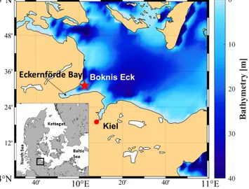
Sampling was performed at BE (Lennartz et al., 2014), whose site is located at the entrance of the Eckernförde Bay (54^◦31.2⁰N, 10^◦02.5⁰E; Fig. 1) in the southwestern Baltic Sea. The BE sampling site has a water depth of 28 m.

Monthly sampling at BE started in 1957, making this sta-

tion one of the longest-operating marine time-series stations worldwide (Lennartz et al., 2014). Riverine inputs are neg- ligible for the Eckernförde Bay, which is dominated by the inflow of North Sea water through the Kattegat and the Great Belt. Seasonal stratification at BE is caused by steep density gradients and usually lasts from March to October with a mixed-layer depth (MLD) of 10–15 m (Hoppe et al., 2013;

Lennartz et al., 2014). During the stratification period, vertical mixing is restricted, and decomposition of organic material by bacteria in the deep layer causes pronounced hypoxia and sporadic anoxia or sulfidic events (Hansen et al., 1999; Lennartz et al., 2014). The main phytoplankton blooms generally occur in spring (February–March). Minor blooms are sporadic in summer (July–August) and always in autumn (September–November) (Smetacek et al., 1984; Smetacek, 1985; Bange et al., 2010). Lennartz et al. (2014) reported an increasingly warming trend of 0.02^◦C yr⁻¹(in 1 and 25 m) at BE for the period from 1957 till 2013. Nutrient concentrations increased until the 1980s in the Baltic Sea, as a result of agricultural over-fertilisation, washing-off, and transport via rain and rivers into the Baltic Sea. The nutrient concentration started to decline due to measures which success- fully reduced anthropogenically caused marine eutrophication in the Baltic Sea (HELCOM, 2018b). However, low- oxygen events (hypoxia or anoxia) have occurred more fre- quently within the last decades in the Baltic Sea and so at BE (Lennartz et al., 2014). Probably, climate warming enhances bacterial activities and respiration (Hoppe et al., 2013) and extends the period of stratification (Liblik and Lips, 2019).

This overrides the effect of decreasing nutrient inputs in the last decades (Lennartz et al., 2014). Overall, the location of BE is ideal for studying the cycling of sulfur compounds such as DMS, DMSP and DMSO in a productive coastal ecosys- tem with strong open-ocean influences, which is affected by pronounced changes in salinity and oxygen.

3 Material and methods 3.1 Sulfur compounds analysis

Monthly sampling of sulfur compounds at BE started in February 2009. Samples were collected bubble-free in 250 mL brown glass bottles. The samples were analysed as soon as possible after returning to GEOMAR’s labora- tory, usually within a few hours after sampling. Back in the lab, out of the 250 mL water sample, three subsamples (10 mL) were immediately taken and gently filtered through a glass fibre filter (GF/F; Whatman; 0.7 µm) attached to a syringe for DMS and dissolved DMSP (DMSP_d) analysis.

We used a purge-and-trap technique attached to a gas chro- matograph equipped with a flame photometric detector (GC- FPD) to measure sulfur compounds as described in Zindler et al. (2012). After DMS was measured, sodium hydroxide (NaOH; Carl Roth) was added to the subsamples to convert

(3)

Figure 1.Location of the Boknis Eck Time Series Station near the entrance of Eckernförde Bay in the southwestern Baltic Sea. The location map was created with the m_map package for MATLAB R2019 (Pawlowicz, 2020).

DMSP into DMS. The conversion was allowed to take place at least overnight before analysis of DMSP_d. Total DMSP (DMSP_t) was measured from the unfiltered alkaline subsamples, and particulate DMSP (DMSP_p) concentrations were calculated by subtracting measured DMS and DMSP_dcon- centrations from measured DMSP_tconcentrations. Dissolved DMSO (DMSO_d) and total DMSO (DMSO_t) samples were measured from the same samples of DMSP_d and DMSP_t measurements by adding cobalt-dosed sodium borohydride (NaBH4; Sigma-Aldrich) right after DMSP analysis to reduce DMSO to DMS. Particulate DMSO (DMSOp) concentrations were calculated by subtracting measured DMSOd

concentrations from measured DMSOtconcentrations. Cali- brations were conducted every measurement day. The mean relative analytical errors for the individual sulfur compounds were generally≤20 %. An overview of the methods used for determining oceanographic parameters – such as water temperature, salinity, dissolved O₂and dissolved nutrients – at BE can be found in Lennartz et al. (2014).

3.2 Phytoplankton analysis

Pigment samples were collected simultaneously with sulfur compound samples at BE. After returning to the lab, 2 L of seawater was filtered through 0.7 µm GF/F glass fibre filters with a pressure of less than 200 mbar to avoid cell breaking. After filtration, the filters were folded and stored in 2 mL microcentrifuge tubes (Eppendorf cups) at

−80^◦C for later analysis. Phytoplankton pigment concentrations from April 2009–December 2011 were analysed using a high-performance liquid chromatography (HPLC; Waters 600 Pump, 474 Scanning Fluorescence Detector, 2996 Pho- todiode Array and 717 Autosampler) technique. Fifty mi- crolitres of an internal standard (canthaxanthin) and 2 mL of

100 % acetone were added, and the pigments were extracted by homogenisation with glass beads in a cell mill (Büh- ler). Samples were centrifuged, and the supernatant was filtered through 0.2 µm PTFE filters (VWR International). Just prior to analysis, the sample was premixed with 1 mol L⁻¹ of ammonium acetate solution in a 1 : 1 (v/v) ratio in the autosampler and injected onto the HPLC system. The pigments were analysed by reverse-phase HPLC, using a VAR- IAN Microsorb-MV3 C8 column (4.6×100 mm) and HPLC- grade solvents (Baker). The gradient was modified after Bar- low et al. (1997). Eluting pigments were detected by ab- sorbance (440 nm). From 2012 on, just prior to analysis, the sample was premixed with 28 mol L⁻¹of tetrabutylam- monium acetate solution in a 1 : 1 (v/v) ratio in the autosampler and injected onto the HPLC system. The pigments were analysed by reverse-phase HPLC, using an Eclipse XDB-C8 column (4.6×150 mm) and HPLC-grade solvents (Baker). The gradient was modified after Van Heukelem and Thomas (2001), and eluting pigments were detected by ab- sorbance (440 nm). Both methods showed a good agreement in a pigment analysis; thus data are comparable before and after 2012.

The taxonomic structure of phytoplankton communities was derived from photosynthetic pigment ratios using the CHEMTAX^®program (Mackey et al., 1996). The input ma- trix of Schluter et al. (2000) and Henriksen et al. (2002) applies for all photosynthetic pigments in this study (Ta- ble S1 in the Supplement). The phytoplankton group composition included diatoms, dinoflagellates, cryptophytes, chrysophytes, chlorophytes, prymnesiophytes and cyanobacteria.

3.3 Mixed-layer depth (MLD)

At 28 m water depth, the BE station is a shallow coastal site.

Compared to other ocean regions, sea surface salinity is quite variable due to the occasional inflow of saline North Sea water (Lennartz et al., 2014). Therefore, a density-based criterion for calculating the MLD is the best approach (Reiss- mann et al., 2009). In order to define the MLD, we used the squared buoyancy frequency (N²), also called stability frequency, which was calculated following Eq. (1):

N²=g ρ

dρ

dz, (1)

by using the water density (ρ), the water depth (z) and the gravity (g). After calculatingN²for all depth profiles of this dataset, the MLD was defined as the minimum depth below 4 m where the criterion ofN²≥10⁻³s⁻²was satisfied. This N² value is low enough to detect a barrier where mixing is mainly suppressed but also high enough not to account for a diurnal surface warm layer, as the MLD is applied for the whole month in which the individual cruises took place.

(4)

4 Results and discussion 4.1 Overview

4.1.1 Environmental setting of BE during 2009–2018 The water temperature varied between 0.42 and 22.15^◦C (Fig. 2a), with a maximum usually in August (14.56^◦C;

Fig. 2b) and a minimum between February (2.88^◦C; Fig. 2b) and March (2.51^◦C; Fig. 2b). The highest water temperature of 22.15^◦C was measured at 1 m water depth in Au- gust 2018, which was during the warmest summer recorded for the Baltic Sea since 1948 (Naumann et al., 2019) and also the second-warmest summer in Germany since 1981 (Zscheischler and Fischer, 2020). The lowest water temperature of 0.42^◦C was measured at 15 m water depth in March 2010. In general, the temperature of the water column at BE increased by 0.02^◦C yr⁻¹during 1957–2013 due to global warming (Lennartz et al., 2014). The salinity in the bottom layer (25 m) ranged from 13.65 to 25.66, with the highest salinity measured in December 2013 (Fig. 2c).

In general, the salinity at 25 m water depth reached its maximum in September (23.09; Fig. 2d), after the stratification period, and its minimum in April (19.64; Fig. 2d), when the water column is well ventilated by wind-driven mixing events.

The bottom salinity showed strong fluctuations, which are caused due to the inflow of saline water originating from the North Sea (Lennartz et al., 2014). For instance, in Decem- ber 2014, a MBI event of highly saline and oxygenated North Sea water occurred after a 10-year stagnation since 2003, as the third-strongest event ever recorded (Fig. 2c, marked with the black arrow; Mohrholz, 2018). Occasionally, the break- up of the late-summer/autumn stratification was caused by upwelling events induced by strong winds, leading to the uni- form distribution of salinity in the entire water column (e.g., in September 2017).

Dissolved oxygen concentrations varied significantly from 0 to 479 µmol L⁻¹(Fig. 2e), with seasonal hypoxic or anoxic events prevailing in the bottom layer (∼20–25 m) in autumn at BE (Fig. 2f). Dissolved phosphate and dissolved inorganic nitrogen (DIN; the sum of nitrate, nitrite and ammonium) concentrations generally displayed regular seasonal variabilities, with higher concentrations in the upper layers during the winter months (December–February) and in the bottom layer during autumn months (September–November; Fig. 2g–j).

The seasonal variability of chlorophyll a (Chl a) concentrations was generally in line with the annual phytoplankton succession at BE previously reported by Smetacek (1985), which is characterised by diatom blooms in spring, minor blooms in summer, dinoflagellate blooms in autumn and a dormancy phase in winter (Fig. 3a and b). During our study, autumn blooms at BE occasionally extended to December, which might have been a result of a longer growing season at higher temperatures in response to climate change (Wasmund et al., 2011). The highest Chl a concentration

(12.4 µg L⁻¹) was measured in the surface layer (1 m) in Oc- tober 2017, accompanied by dinoflagellates dominating the autumn bloom.

4.1.2 Sulfur compounds

DMSP_p concentrations were up to 103.5 nmol L⁻¹ with an average of 9.2±13.3 nmol L⁻¹ in the water column, and DMSP_d concentrations reached up to 42.7 nmol L⁻¹ with an average of 3.0±4.1 nmol L⁻¹. The highest concentration of DMSP_pwas measured at 15 m depth in April 2015.

Generally, the seasonal and spatial patterns of DMSPp and DMSPd followed that of Chl a, which was enhanced in spring (February–April) and autumn (September–October) in the upper layer (∼1–15 m) and decreased with increasing depth (Fig. 3a–f). The overall mean ratio of DMSPp: DMSPd

was 4.5±8.5, indicating that DMSP_p was generally dominant in the DMSP pool at BE. This is in line with the results reported by Speeckaert et al. (2018) from the coastal areas in the southern North Sea. DMSO_pconcentrations were up to 208.4 nmol L⁻¹with an average of 11.3±20.7 nmol L⁻¹ in the water column. DMSO_d concentrations were up to 70.3 nmol L⁻¹ with an average of 7.9±8.2 nmol L⁻¹. The highest DMSO_p concentration was measured at 1 m depth in the same sampling month as DMSP_p. The seasonal and spatial distributions of DMSO_p and DMSO_d were similar to DMSP (Fig. 3i–l). The mean ratio of DMSOp: DMSOd

was 1.7±2.4, suggesting less dominance of the ratio of DMSOpto DMSOdin contrast to DMSP. Overall, our study is consistent with the results reported in Hatton and Wil- son (2007) that DMSPd was very low compared to DMSPp

while DMSO_d could exceed the sum of DMS and DMSP_d concentrations in the seawater. Additionally, significant correlations between DMSP_p and DMSO_p as well as DMSP_t and DMSO_t (Table 1) in this study are in agreement with those reported in previous studies. This suggests that both sulfur compounds might share the same source in the seawater, and they are subject to close cycling of production and consumption where the composition of the plankton community plays a prominent role (Simo et al., 1997; Zindler et al., 2013).

The overall mean DMS concentration was 1.3±1.8 nmol L⁻¹ in the water column, with the highest concentration of 20.5 nmol L⁻¹ measured at 1 m depth in April 2015. The mean concentration of DMS in the mixed layer was 1.7±2.0 nmol L⁻¹, which is slightly lower compared to the mean DMS concentration of 2.7±2.0 nmol L⁻¹for the Baltic Sea (53–66^◦N, 10–30^◦E) retrieved from the Global Surface Seawater DMS Database (http://saga.pmel.noaa.gov/dms, last access: 19 Novem- ber 2020), including DMS data from Leck et al. (1990) and Leck and Rodhe (1991). DMS concentrations measured at the entrance of Himmerfjärden Fjord (western Baltic Sea) from January 1987 to June 1988 ranged from 0.1 to 6.3 nmol L⁻¹ with an average of 1.5±1.3 nmol L⁻¹

(5)

Figure 2.Monthly and mean seasonal distributions of temperature(a, b), salinity(c, d), dissolved O₂(e, f), phosphate(g, h)and dissolved inorganic nitrogen(i, j)at BE during 2009–2018. Please note that in the left panels the blank areas are due to data gaps caused by cancellations of the research cruises, and the dashed lines indicate January of each year. Black dots (c)and the black line(d) indicate monthly and mean seasonal distributions of the mixed-layer depth, respectively. The black arrows (c)indicate the major Baltic inflow (MBI) events in November 2010 and December 2014. Time–depth Hovmöller diagrams were generated with MATLAB; note that the colour coding in panels(g)and(i)is shown on a natural logarithmic scale.

(Leck et al., 1990), which is in line with our study. Sur- face DMS was also measured in the Baltic Sea and the Kattegat–Skagerrak (the connection between the Baltic Sea and the North Sea) to be 1.3±0.8 and 2.4±0.9 nmol L⁻¹ in July 1988, respectively (Leck and Rodhe, 1991), the former of which was comparable and the latter of which was higher compared to this study. However, statistical results from Leck and Rodhe (1991) indicated that no single factor, such as salinity or certain phytoplankton species, could account for these higher concentrations of DMS in the Kattegat–Skagerrak. Leck and Rodhe (1991) suggested that increased eutrophication of coastal regions may result in a net positive effect on DMS production in the Baltic Sea.

The study from Orlikowska and Schulz-Bull (2009) in the Bay of Mecklenburg (southern Baltic Sea) showed DMS concentration in the range from<0.3 nmol L⁻¹in Novem- ber 2008 up to 120 nmol L⁻¹in May 2008. Considering that the concurrent Chl a concentrations from phytoplankton

were only 2–4 µg L⁻¹, Orlikowska and Schulz-Bull (2009) proposed that macroalgae could also contribute significantly to the DMS production. A comparison with data from other coastal time-series stations (Table 2) reveals that mixed-layer DMS concentrations at BE are generally comparable to those measured at other time-series stations in coastal regions like in the Baltic Sea, the Mediterranean Sea or the Indian Ocean.

DMSP_t concentrations from BE are in the same range as the concentrations reported from the NW Mediterranean Sea and the western English Channel, but they are lower than those reported from the southern North Sea (including the Belgian and Dutch coasts), the Revellata Bay (Gulf of Calvi, Mediterranean Sea) and the coast off Goa (eastern Arabian Sea, Indian Ocean). DMSO_t concentrations at BE were generally in the same range as reported from other time-series sites except for the extremely high DMSO_t concentrations measured at the coast of Belgium (southern North Sea). The obvious high variabilities in the range of

(6)

DMSP or DMSO concentrations are most probably resulting from the interplay of various factors such as differences in sampling periods/frequency, the prevailing phytoplankton/bacteria community composition and succession, and the eutrophication status as well as the occurrence of anoxic events.

4.2 Temporal trend analysis

Temporal trend analysis was calculated by anomaly detec- tion via subtracting the overall monthly mean (2009–2018) from the individual monthly mean, followed by smoothing with a 12-point moving average, which was used to reduce the effects of the seasonal as well as annual cycles on the temporal trend. Temperatures showed increasing trends in the mixed layer and the bottom layer (Fig. 4a) during our study. The trends were 0.2^◦C yr⁻¹and 0.1^◦C yr⁻¹(Table 3) in the mixed layer and the bottom layer, respectively. Our result is consistent with the study by Belkin (2009), who reported a post-1987 warming rate in the Baltic Sea exceeding 1.0^◦C decade⁻¹. A less pronounced trend of 0.02^◦C yr⁻¹(at 1 and 25 m) during 1957–2013 was reported by Lennartz et al. (2014). This disagreement may arise from the fact that the result reported by Lennartz et al. (2014) covers a much longer study period and there might be an acceleration trend of increasing temperature starting around 2014 (Rahmstorf et al., 2017). Salinity in the bottom layer (25 m; Fig. 4b) did not show significant trends in our study, which is in agreement with Lennartz et al. (2014). Additionally, there is no trend of dissolved oxygen in the bottom layer (Fig. 4b), which is different to the trend computed by Lennartz et al. (2014), who reported that bottom O₂ concentrations were decreasing over 56 years. Again, this difference is attributed to the much shorter observation period of our study compared to Lennartz et al. (2014). Dissolved inorganic nitrogen (Fig. 4c) and phosphate (Fig. 4d) showed slightly increasing trends of 0.5 and 0.2 µmol L⁻¹yr⁻¹(Table 3) in the bottom layer, but similar trends were not observed or apparent in the mixed layer. The decreasing trends for nutrients (in 1 and 25 m) at BE reported by Lennartz et al. (2014) are due to a reduction of nutrient inputs to the Baltic Sea to improve the eutrophication status of the Baltic Sea (HELCOM, 2018a). This is consistent with Kuss et al. (2020), who reported a decline in DIN from 1995–2004 and total phosphate from 2005–

2009 in the Belt Sea with no significant changes thereafter.

In our study, the increasing trends of nutrients at 25 m coin- cided with increasing temperature as well as more frequent hypoxic/anoxic events (i.e. ongoing deoxygenation) at 25 m.

Increasing temperature favoured bacteria decomposing activities beneath the thermocline due to more pronounced water column stratification, supporting their remineralisation and, thus, leading to more consumption of dissolved oxygen, and releasing more nutrients in the bottom layer (Hoppe et al., 2013; Lennartz et al., 2014). Thus, the increasing nutrient concentrations are not a general eutrophication of the water

column but a natural effect limited within the bottom layer.

Chlaconcentration (Fig. 4e) showed an increasing trend of 0.2 µg L⁻¹yr⁻¹ (Table 3) in the mixed layer, which is primarily driven by high concentrations in 2017, similar to the variability of the sum of fucoxanthin (a marker pigment for diatoms) and peridinin (a marker pigment for dinoflagellates;

Fig. 4i).

DMSP_t concentrations (Fig. 4f) showed a slightly decreasing trend both in the mixed layer (−0.9 nmol L⁻¹yr⁻¹) and in the bottom layer (−0.3 nmol L⁻¹yr⁻¹; Table 3), as opposed to the upward trends of Chl a in the mixed layer and temperature both in the mixed and bottom layer. A similar decreasing trend in the mixed layer (−9.2 ng L⁻¹yr⁻¹) was detected for the sum of the pigments 19⁰-hexanoyloxyfucoxanthin (19⁰-hex, a marker pigment for prymnesiophytes) and 19⁰-butanoyloxy-fucoxanthin (19⁰- but, a marker pigment for chrysophytes; Fig. 4i). This indicates that the general trend of DMSP_t concentrations in the mixed layer might be primarily controlled by the productiv- ity of chrysophytes and prymnesiophytes (see also Table 1).

The decreasing trend for DMS (−0.1 nmol L⁻¹yr⁻¹; Fig. 4g) generally followed the pattern of DMSP_tin the mixed layer and indicates that DMSP cleavage might play a dominant role in the production of DMS (see Table 1). Although no significant trend was observed for DMSO_t(Fig. 4h), its general variability over time was similar to those of DMSP_tand DMS in the mixed layer. The decreasing trend observed for DMSPt at 25 m might be mainly attributable to the corresponding sinking particles from the mixed layer, as no trends were observed for Chlaor other algae groups at 25 m.

As a statistical test to decipher significant monotonic long- term trends in time series, the Mann–Kendall test (MKT) was also applied to detect the temporal trends of the individual months. However, no significant trends were observed for any of the dimethylated sulfur compounds by the MKT in our study.

4.3 Influence of extreme events at BE on the sulfur compounds

4.3.1 The major Baltic inflow events

MBI events carry large amounts of oxygen-rich saline North Sea water into the Baltic Sea (Mohrholz et al., 2015) and can transport phytoplankton species originating from the North Sea into the Baltic Sea (Olenina et al., 2010). A MBI event lasted for 1 month in 2014 and was detected in the Eck- ernförde Bay by elevated sea levels after an outflow period, which indicated that its inflow began on 10 December 2014 (Ma et al., 2020). Therefore, the sampling at BE on 16 De- cember 2014 took place during the MBI period. Our results show that the sulfur compound concentrations in the water column in December 2014 and in January 2015 were low and similar to the overall mean concentrations of sulfur compounds in December/January for the period 2009–2018, in-

(7)

Table 1.Spearman’s rank correlation coefficients of correlations of all sulfur compounds with several ambient parameters, as well as algae groups in the mixed layer at BE during 2009–2018. Only datasets were used for which all environmental parameters (n=85), phytoplankton data (n=61 for diatoms and dinoflagellates,n=48 for chrysophytes, andn=35 for prymnesiophytes) were available, and data were averaged for the mixed layer. Bold numbers indicate that a correlation is significant at the 0.01 level (two tailed). Diat, dino, prym and chryso stand for diatoms, dinoflagellates, prymnesiophytes and chrysophytes, respectively. N : P ratios stand for the ratio of the sum of nitrate, nitrite and ammonium to phosphate.

DMS DMSP_t DMSP_p DMSP_d DMSO_p DMSO_d DMSO_t Chla −0.31 0.19 0.11 0.04 0.29 −0.11 0.2

Temperature 0.41 0.11 0.14 −0.12 0.26 0.12 0.24

Salinity −0.19 0.08 −0.04 −0.05 −0.09 −0.11 −0.08

N : P −0.15 −0.21 −0.08 −0.04 −0.12 −0.04 0.14

Diat −0.04 −0.05 −0.13 0.16 −0.25 −0.24 −0.27

Dino 0.10 0.09 0.19 −0.26 0.2 0.06 0.19

Prym 0.25 0.38 0.47 0.14 0.35 0.30 0.34

Chryso 0.32 0.44 0.37 0.29 0.28 0.25 0.32

DMSO_t 0.35 0.79 0.72 0.43 0.86 0.75

DMSO_d 0.35 0.57 0.48 0.61 0.41

DMSO_p 0.20 0.72 0.74 0.26

DMSP_d 0.26 0.53 0.27

DMSP_p 0.44 0.91

DMSPt 0.42

dicating that the MBI in December 2014 did not influence the concentrations of sulfur compounds at BE directly. Rel- atively higher DIN and dissolved phosphate concentrations (Fig. 2g and i) were measured in December 2014, and this would be assumed to trigger a more significant spring bloom in the next year and, therefore, higher sulfur compound concentrations. Indeed we measured higher concentrations of sulfur compounds in March and April 2015; however, this is probably attributable to the unusually higher proportion of prymnesiophytes of the phytoplankton community (see Sect. 4.4), and this high fraction of prymnesiophytes was not supposed to be caused by the rich nutrients accumulated in December 2014. The peak of the spring bloom in 2015 could not be identified considering moderate Chla concentrations in February (1.0 µg L⁻¹) and March (2.0 µg L⁻¹), but a sub- stantial decrease of nutrients occurred between February and March 2015. Concentrations of DIN and dissolved phosphate stayed high until February 2015. Subsequently, DIN concentrations decreased from 8.0 µmol L⁻¹ in the mixed layer on 23 February to 0.1 µmol L⁻¹ on 17 March, with dissolved phosphate decreasing from 0.7 to 0.1 µmol L⁻¹in the same case. Depleted nutrients in March suggested the spring bloom peak between the sampling date in Febru- ary and in March 2015 was apparently not captured by our monthly measurements and underlines the necessity of frequent sampling. As a minor algae group at BE, prymnesiophytes tend to accumulate towards the end of spring diatom blooms in oligotrophic conditions (Veldhuis et al., 1986), and this was confirmed by the decreasing concentration of silicate from 12.5 µmol L⁻¹in the mixed layer in February 2015 to 2.2 µmol L⁻¹in March, which is the limiting growth factor of

diatoms. Therefore, we conclude that the accumulation of nutrients had been consumed by diatoms between February and March before prymnesiophytes formed the bloom. However, the much-higher-than-usual relative abundance of prymnesiophytes in March and April 2015 (see Fig. 5a) might have been transported to BE by the saline water from the North Sea, where prymnesiophytes are abundant (Speeckaert et al., 2018).

Another relatively weak MBI occurred in late autumn 2010 (Mohrholz et al., 2015), and we measured elevated salinity concentrations in November 2010 at BE (see Fig. 2c).

Subsequently, above-average concentrations for DMS (1.9–

3.7 nmol L⁻¹), DMSP_p (50.9–84.5 nmol L⁻¹) and DMSO_p (32.2–40.6 nmol L⁻¹) were measured in spring bloom during February–April 2011, coinciding with the exceptionally higher relative abundance of chrysophytes in the mixed layer (see Fig. 4). We assume that this chrysophyte was rather new and uncommon, only occurring in the Kiel Bight and Bay of Mecklenburg (Wasmund et al., 2012). Therefore, it is possible that this uncommon chrysophyte was brought into the western Baltic Sea via saline waters in autumn 2010 and bloomed in spring 2011, resulting in high concentrations of DMSP and thus DMS(O) at BE.

Overall, enhanced DMSPp concentrations (>50 nmol L⁻¹) measured during the spring bloom in 2011 and 2015 both followed after the MBI events in winter and comprised newly formed phytoplankton groups not common at BE. Therefore, we hypothesise that MBI was likely to influence sulfur compound concentrations by introducing new phytoplankton species which are good DMSP producers.

(8)

Figure 3.Monthly and mean seasonal distributions of chlorophylla(a, b), DMSP_p(c, d), DMSP_d(e, f), DMS(g, h), DMSO_p(i, j)and DMSO_d(k, l)at BE during 2009–2018. Black dots(g)and the black line(h)indicate monthly and mean seasonal distributions of the MLD, respectively. The black arrows(g)indicate the major Baltic inflow (MBI) events in November 2010 and December 2014. The red arrows indicate elevated concentrations of DMS under hypoxia/anoxia in 2009, 2010, 2016 and 2018. In 2009, DMSO data were only available from April to July. Time–depth Hovmöller diagrams were generated with MATLAB, and concentrations shown in the left panels are given on a natural logarithmic scale.

4.3.2 Low-oxygen events

Hypoxia in this study is defined as dissolved O2 concentrations being below 62.5 µmol L⁻¹ (i.e. 2 mg L⁻¹), according to Vaquer-Sunyer and Duarte (2008). Low-oxygen events (hypoxia/anoxia) are usually observed in the bottom layer at BE, as a result of long-lasting stratification and enhanced remineralisation of organic matter (Lennartz et al., 2014). During seasonal hypoxic/anoxic conditions (see Fig. 3e), elevated concentrations of DMS (up to 4.19 nmol L⁻¹) were measured in the bottom layer in Au- gust 2009, August–October 2010, September 2016 and September 2018 (see Fig. 3g). These elevated DMS concentrations (2.3±1.4 nmol L⁻¹) in the bottom layer (20–

25 m) were generally comparable to or lower than those

found in the mixed layer (0–5 m; 3.4±2.2 nmol L⁻¹) but higher than those in the overlying water layers (15–20 m;

1.2±1.2 nmol L⁻¹). Shenoy et al. (2012) reported extremely high concentrations of DMS (up to 442 nmol L⁻¹) as well as enhanced DMSP_t, DMSO_tand methanethiol concentrations in the bottom layer during an anoxic event at Candolim Time Series Station (CaTS) off Goa, west India, in September 2009 and suggested that this unusually high DMS concentration might result from a combination of sources such as DMSP cleavage, DMSO reduction, methylation of methanethiol and hydrogen sulfide under anoxic conditions. Later on, Bepari et al. (2020) observed high concentrations of DMS (233 nmol L⁻¹) in the bottom layer during an anoxic event at CaTS in September 2013 and assumed that sediments might also be an important source of DMS, in addition to the

(9)

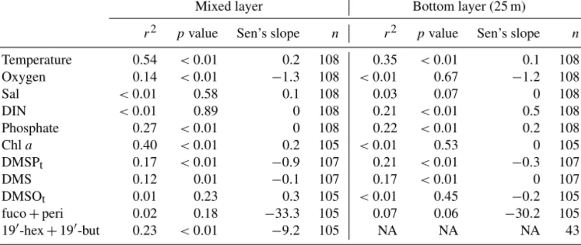
Table 2.Surface sulfur compound concentrations from coastal time-series studies.

Region Period of

sampling

Sampling frequency

DMS avg range (min–max)

DMSP_t avg range (min–max)

DMSO_t range (min–max)

Chla avg range (min–max)

Reference

Boknis Eck Time Series Station, the southwest Baltic Sea

Apr 2009–

Dec 2018

Monthly 1.7^a

0.1–12.2^a

18.5^a 1.4–85.4^a

31.1^a 2.5–209.8^a

2.1^a 0.3–10.8^a

This study

Station B1, Himmerfjär- den Fjord, the west Baltic Sea

Jan 1987–

Jun 1988

Weekly in spring, biweekly in summer and monthly in winter

1.51 0.1–6.3

nm nm ng

<1–12

Leck et al. (1990)

Heiligendamm station, Bay of Mecklenburg, the Baltic Sea

Jan–Nov 2008 Weekly ng

up to∼120

nm nm ng

∼1–7

Orlikowska and Schulz-Bull (2009) The southern North Sea Feb–Oct 1989 Monthly 3.92

0.1–>50 ng up to 450

nm ng

up to 35

Turner et al.

(1996) The Belgian coastal zone,

the North Sea

Jan–Dec 2016 Bimonthly from Feb to Jun and monthly for the rest

ng up to 250

ng up to 1740^b

ng up to 620

ng up to 36

Speeckaert et al.

(2018)

Coast of Den Helder, the Netherlands

Nov 1991–

Nov 1992 and Jan–Jun 1993

Biweekly in 1991 and 1992, more frequent in 1993

ng 0–18

ng 7–>1500^b

nm ng

0–65

Kwint and Kramer (1996)

Station L4, the western English Channel

May–Oct 2014 Weekly 5.1

up to 17 ng

∼10–100 ng 2.3–102

ng

∼0.1–2.4

Dixon et al.

(2020) Toulon Bay, the NW

Mediterranean Sea

Jan–Dec 1997 Monthly 9.8

3.6–21.03

nm nm ng

0.2–2.5

Despiau et al.

(2002) The NW Mediterranean

Sea

Jan 2003–

Jun 2004

Monthly ng

∼0.5–19 ng

∼10–71.7^b ng

∼0–24.2^b ng

∼0.4–2.8

Vila-Costa et al.

(2008) Revellata Bay,

Gulf of Calvi

Apr 2015–

Jul 2016

Weekly to biweekly

nm 130^c

62–205^c

4.9^c 1.5–8.6^c

ng Richir et al.

(2019) The Zuari estuary off Goa Dec 1999–

Jan 2001

Monthly 5.8

0.3–15.4

68.3 0.8–415.9

nm ng

up to∼10

Shenoy and Patil (2003)

Candolim Time Series Station, coast off Goa

Sep 2009–

Dec 2013

Monthly 22.5

0.5–442 24 0.4–252

27.8 0.6–185.9

ng 0.1–14.4

Bepari et al.

(2020) Rothera Time Series

Station, Ryder Bay, West Antarctic

Sep 2012–

Mar 2017

2–3 times per week in austral summer and less frequency in austral winter

3.7 0.1–170

ng ng ng Webb et al.

(2019)

aAveraged for the mixed layer.^bGiven as DMSPpor DMSOp; ng and nm stand for not given and not measured, respectively.^cGiven as µmol g⁻¹_fw. The units of sulfur compounds and Chlaare given as nmol L⁻¹and µg L⁻¹, respectively.

breakdown of simultaneously high concentrations of DMSP_t (206–252 nmol L⁻¹) in the water column. However, in the case of BE, concentrations of DMSP_t (4.7±4.9 nmol L⁻¹) or DMSO_t (4.1±2.2 nmol L⁻¹) measured in the bottom layer during hypoxia/anoxia events were lower than those in the mixed layer (DMSP_t: 20.6±8.1 nmol L⁻¹; DMSO_t: 32.4±17.0 nmol L⁻¹) or the overlying water layer (DMSP_t: 11.9±4.1 nmol L⁻¹; DMSO_t: 17.7±11.6 nmol L⁻¹), which

indicates that DMSP cleavage and DMSO reduction processes are unlikely to account for the main fraction of DMS production. Therefore, it is reasonable to assume that these elevated concentrations of DMS in the bottom layer might have been at least in part released from the sediments and might originate from the methylation of methanethiol and/or hydrogen sulfide (Nedwell et al., 1994; Song et al., 2020).

This assumption is in agreement with Bertics et al. (2013),

(10)

Figure 4.Temporal trends of anomalies of temperature (^◦C)(a), dissolved oxygen (µmol L⁻¹) and salinity(b), dissolved inorganic nitrogen (DIN; µmol L⁻¹)(c), phosphate (µmol L⁻¹)(d), Chla(µg L⁻¹)(e), DMSPt(nmol L⁻¹)(f), DMS (nmol L⁻¹)(g), DMSOt(nmol L⁻¹)(h), and the sum of pigment concentrations of fucoxanthin (fuco) and peridinin (peri) (ng L⁻¹) and 19⁰-hexanoyloxyfucoxanthin (19⁰-hex) and 19⁰-butanoyloxy-fucoxanthin (19⁰-but) (ng L⁻¹)(i). The shaded areas indicate 95 % confidence intervals. Note that gaps were filled by linear interpolation in the case of one or two missing months in a row, and large gaps between August and December 2009 in DMSO_t(h)were filled by replacement with the median of the corresponding month.

who reported increased sulfate reduction activities between August and November 2010 in the surface sediment at BE, which would favour the production of hydrogen sulfide and further methanethiol. Additionally, groundwater discharge in Eckernförde Bay may also have an indirect impact on DMS production by increasing sulfate reduction activities (Buss- mann et al., 1999). However, elevated DMS concentrations

in the bottom layer were not always measured simultaneously with low-oxygen events. In only 5 out of 18 sampling months, we observed elevated DMS concentrations together with low-oxygen events (see Fig. 3g and e). Therefore, we speculate that there is a switch between DMS generation and removal processes in the sediments (Kiene, 1988; Nedwell et al., 1994), which needs to be further investigated at BE.

(11)

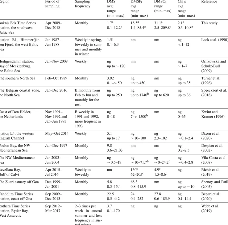
Table 3.Statistics of the linear regression of the temporal trends for the anomalies of temperature (^◦C), dissolved oxygen (µmol L⁻¹), salinity, dissolved inorganic nitrogen (DIN; µmol L⁻¹), phosphate (µmol L⁻¹), Chl a(µg L⁻¹), DMSP_t (nmol L⁻¹), DMS (nmol L⁻¹), DMSOt(nmol L⁻¹), the sum of pigments of fucoxanthin (fuco) and peridinin (peri) (ng L⁻¹), and 19⁰-hexanoyloxyfucoxanthin (19⁰-hex) and 19⁰-butanoyloxy-fucoxanthin (19⁰-but) (ng L⁻¹).r²: coefficient of determination in the simple linear regression calculated by the monthly individual time-series parameters. Sen’s slope: median slope present in time series (yr⁻¹) according to Sen (1968).

Mixed layer Bottom layer (25 m)

r² pvalue Sen’s slope n r² pvalue Sen’s slope n

Temperature 0.54 <0.01 0.2 108 0.35 <0.01 0.1 108

Oxygen 0.14 <0.01 −1.3 108 <0.01 0.67 −1.2 108

Sal <0.01 0.58 0.1 108 0.03 0.07 0 108

DIN <0.01 0.89 0 108 0.21 <0.01 0.5 108

Phosphate 0.27 <0.01 0 108 0.22 <0.01 0.2 108

Chla 0.40 <0.01 0.2 105 <0.01 0.53 0 105

DMSP_t 0.17 <0.01 −0.9 107 0.21 <0.01 −0.3 107

DMS 0.12 0.01 −0.1 107 0.17 <0.01 0 107

DMSO_t 0.01 0.23 0.3 105 <0.01 0.45 −0.2 105

fuco+peri 0.02 0.18 −33.3 105 0.07 0.06 −30.2 105

19⁰-hex+19⁰-but 0.23 <0.01 −9.2 105 NA NA NA 43

NA – not available.

4.4 Relationships between the sulfur compounds and phytoplankton groups

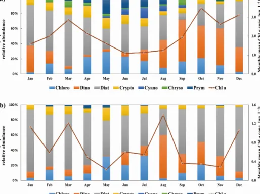
In general, phytoplankton composition and succession (Fig. 5a) at BE were similar to previous studies from the Baltic Sea with a recurrent pattern of diatoms dominating the bloom in spring (February–April) and summer (June–

August) followed by dinoflagellates in autumn (September–

November) (Smetacek, 1985; Wasmund et al., 2008). Di- atoms were the most dominant phytoplankton group at the Boknis Eck station, especially during the spring bloom, and reached their maximum in March. The fraction of diatoms gradually decreased in April and May, whereas the fractions of prymnesiophytes, cryptophytes and chlorophytes increased, accompanied by the development of cyanobacteria.

Minor summer blooms most commonly occurred in August below the surface water (e.g., in 15 or 20 m) at BE, as a result of stratification which restricted the bottom nutrients supply to the surface layer (Fig. 5b). The autumn/winter bloom period (September–December) was mainly composed of a mix- ture of dinoflagellates and diatoms or a succession of these two algae groups. Overall, diatoms and dinoflagellates were the most common phytoplankton groups at BE.

4.4.1 Relationship between sulfur compounds and phytoplankton groups

Positive correlations were found between chrysophytes and DMSP_p as well as prymnesiophytes and DMSP_p in the mixed layer (Table 1). Enhanced concentrations of DMSP_p (>50 nmol L⁻¹) were associated with the high relative abundance of chrysophytes (25–62 % between February and April 2011) and prymnesiophytes (29–56 % in March and

April 2015) in the mixed layer. Reports from Wasmund et al. (2012, 2016) confirmed that these two algae groups were higher in their abundances in the years 2011 and 2015 in the western Baltic Sea, respectively. Our results suggest that these two algae groups might be the main producers of DMSP in the mixed layer at BE, and this is in agreement with the results of the previous studies of Keller et al. (1989) and Belviso et al. (2001), who found that chrysophytes and prymnesiophytes can be significant DMSP producers in general. No correlation was found between dinoflagellates and DMSP_p in the mixed layer (Table 1). In previous studies, massive dinoflagellate blooms were reported to be closely coupled with high concentrations of DMSP. For example, the highest DMSP concentration (4240 nmol L⁻¹) reported so far was found tightly linked to elevated abundance of Akashiwo sanguinea(Kiene et al., 2019). This could be attributed to that the ability to produce DMSP is considerably variable among different genus and species (Keller et al., 1989). Hence, low or high DMSP concentrations during dinoflagellate blooms are dependent on the dominant species or composition. Typically,Ceratiumwas one of the most common genera during dinoflagellate-dominant autumn blooms in the western Baltic (Wasmund et al., 2015). However, the ability of Ceratium spp. to produce DMSP is rather weak compared to other species or genera of dinoflagellates (Keller et al., 2012). The discrepancy between maximum Chlaconcentration (12.4 µg L⁻¹) dominated by dinoflagellates and the DMSPpconcentrations (25.2 nmol L⁻¹) at 1 m depth in October 2017 might be attributed toCeratium tripos being the dominative species during dinoflagellate blooms (Wasmund et al., 2018), which might be of minor importance for the DMSP pool at BE. Positive correlations were

(12)

found between prymnesiophytes and DMSOp(Table 1) in the mixed layer. Similar to DMSP_p, enhanced concentrations of DMSO_p(>80 nmol L⁻¹) were measured with high propor- tions of prymnesiophytes in March and April 2015, suggesting prymnesiophytes might also be important producers of DMSO at BE. Overall, despite prymnesiophytes and chrysophytes being good producers of DMSP(O) at BE, the seasonal distributions of DMSP(O)_pin the mixed layer followed that of Chlainstead of specific algae groups in terms of their large interannual/seasonal variabilities (Fig. 6a).

DMSP_p and DMSO_p concentrations in the bottom layer (25 m) were generally low throughout the year except for August. We observed a higher relative abundance of dinoflagellates at 25 m in August (Fig. 6b), which were probably more adapted to seawater stratification (Estrada et al., 1985). The ability of dinoflagellates to migrate vertically helps them to cross the pycnocline to get access to the nutrients which accumulate below the mixed layer during the periods of the pronounced summer stratification. Better nutrient access can promote the metabolic activity and thus the DMSP production within dinoflagellates. Also, as mentioned above, the ability to produce DMSP among dinoflagellates varies substantially. For instance, the elevated concentrations of DMSP_pat 25 m in August 2011, 2012 and 2014 might result from the observed high biomass ofAlexandriumspp. in the phytoplankton community in the Bay of Kiel (Wasmund et al., 2012, 2013, 2015), which is generally considered as a good DMSP producer in dinoflagellates (Caruana and Ma- lin, 2014). Therefore, the relationship between dinoflagellates and DMSP at BE may not be well represented at the class levels (Griffiths et al., 2020).

DMS concentrations were negatively correlated with Chla concentrations and poorly correlated with any phytoplankton groups (Table 1) in the mixed layer at BE. Similar cases for these correlations have been reported in many studies (Townsend and Keller, 1996; Toole and Siegel, 2004) due to the complex production and removal processes of DMS.

4.4.2 Predictive algorithms

An algorithm which is able to predict DMS concentrations and thus its emission to the atmosphere could potentially help to improve climate models (Simó and Dachs, 2002; Wang et al., 2020). To reproduce and predict DMS(P) concentrations, parameters such as Chla, temperature, solar radiation or nutrients are often used. To this end, we tested three predictive algorithms suggested by Simó and Dachs (2002) (S02) and Watanabe et al. (2007) (W07) as well as Nagao et al. (2018) (N18) to predict DMS concentrations (S02 and W07) and the DMSP_p: Chlaratios (N18) in the surface layer (5 m) at BE.

The algorithm proposed by Simó and Dachs (2002) makes use of the MLD and the MLD : Chl a ratio to predict DMS concentrations in the mixed layer. Watanabe et al. (2007) proposed an empirical equation for the prediction of sea surface DMS concentrations by combining sea surface temper-

atures, nitrate and latitude. No significant correlations were found between the measured DMS concentrations from this study and the predicted DMS concentrations by applying the S02 and W07 algorithms. Possible reasons might be that S02 was derived from a global dataset from coastal and open- ocean regions and that W07 was based on a dataset from the open North Pacific Ocean, which is in contrast to our coastal dataset.

The Fp ratio was first proposed by Claustre (1994) and was defined as a trophic status ratio, based on the ratio of integrated concentrations of fucoxanthin and peridinin to the sum of the integrated concentrations of diagnostic pigments.

Then, inspired by Aumont et al. (2002), Nagao et al. (2018) proposed new Fp ratios representing the fractions of major and minor DMSP producers in the phytoplankton community to predict the DMSPp: Chlaratios by using phytoplankton pigments:

Fp(high)= 19⁰-hex+19⁰-but+peridinin

Ppigments , (2)

Fp(low)=

fucoxanthin+zeaxanthin +alloxanthin+Chlb

Ppigments , (3)

where “P

pigments” stands for the sum of fucoxanthin, peridinin, 19⁰-hex, 19⁰-but, zeaxanthin, alloxanthin and Chlb.

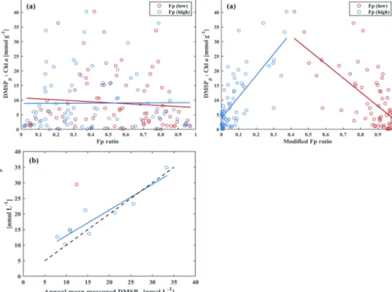
However, results from Eqs. (1) and (2) did not work well with the DMSP_p: Chlaratios from our study (Fig. 7a); nei- ther the Fp (high) nor the Fp (low) ratios correlated well with the DMSPp: Chlaratios at 5 m. As discussed above, the ability to produce DMSP for dinoflagellates was generally low at BE in the mixed layer. Therefore, we modified Eqs. (2) and (3) by moving peridinin from Fp (high) to Fp (low) as fol- lows:

New Fp(low)=

fucoxanthin+zeaxanthin +alloxanthin+Chlb+peridinin

Ppigments , (4)

New Fp(high)=19⁰-hex+19⁰-but

Ppigments . (5)

Significantly negative and positive correlations were found between the DMSPp: Chl a ratios and the new Fp (high) and new Fp (low) ratios at 5 m, respectively (Fig. 7b). The newly defined Fp (high) and Fp (low) represent the measured DMSPp: Chlaratios accurately, additionally showing that DMSPp is mainly driven by the phytoplankton community. Then annual mean DMSP_p concentrations at 5 m were simulated by annual mean 19⁰-hex, 19⁰-but and Chla concentrations, and they were compared to the measured concentrations (Fig. 7c). Our simulated DMSP_p is in good agreement with our measured DMSP_p except for the year 2017 (the red dot in Fig. 7c). In 2017, we measured the most pronounced spring (Chl a: 9.0 µg L⁻¹) and autumn blooms (Chla: 12.4 µg L⁻¹) of the entire observation period.

The blooms were dominated by diatoms and dinoflagellates,

(13)

Figure 5.Monthly mean phytoplankton composition at the Boknis Eck station from 2009 to 2018 based on the result of CHEMTAX. The same months of each year were averaged. Please note that pigment samples are available from April 2009 until December 2018. The values are averaged for the mixed layer(a)and bottom layer(b). Chloro stands for chlorophytes, dino stands for dinoflagellates, diat stands for diatoms, crypto stands for cryptophytes, cyano stands for cyanobacteria, chryso stands for chrysophytes and prym stands for prymnesiophytes. The red lines indicate monthly mean Chlaconcentrations for the mixed layer and bottom layer.

Figure 6. (a)Monthly mean DMSP_p, DMSO_pand Chlaconcentrations in the mixed layer during 2009–2018 at BE.(b)Monthly mean DMSPp, DMSOpconcentrations and relative abundance of dinoflagellates at 25 m during 2009–2018 at BE. Error bars represent standard errors of the mean of the samples.

which led to maximum annual mean Chla but low DMSP_p concentrations.

5 Conclusions

We present a unique and comprehensive time-series study of sulfur compounds (DMS, DMSP and DMSO) at the Boknis Eck Times Series Station, located in the Eckernförde Bay (SW Baltic Sea), from 2009 to 2018. Distinct interannual and seasonal variabilities of sulfur compounds were tightly

linked to the phytoplankton composition at BE. DMSP_pand DMSO_p concentrations were generally enhanced in spring and autumn in the mixed layer, following the pattern of Chla.

Mixed-layer DMSPtand DMS did not follow the increasing trends of the mixed-layer temperature and Chla during the 10-year observation period. The main DMSP and DMS producers – namely, prymnesiophytes and chrysophytes (represented by their marker pigments 19⁰-hex and 19⁰-but, respectively) – decreased in their total abundances over the 10 years.

(14)

Figure 7. (a)DMSPp: Chlavs. Fp ratio (from Nagao et al., 2018) at 5 m for the period 2009–2018.(b)DMSPp: Chlavs. modified Fp ratio (new Fp ratio) at 5 m for the period 2009–2018: blue open circles depict Fp (high) (y=72.90x+3.78,R²=0.54,p <0.01,n=65), and red open circles depict Fp (low) (y= −48.33x+51.35,R²=0.46,p <0.01,n=65).(c)Annual mean measured DMSPpvs. annual mean predicted DMSP_pconcentrations at 5 m for each year during 2009–2018:y=0.82x+4.78,R²=0.86,p <0.01,n=9. Note that the red open circle was not included in the linear regression line (blue), and the dash line indicates the identity (1 : 1) line.

MBI events, which occurred in November 2010 and De- cember 2014 at BE, might have influenced sulfur compound concentrations by introducing uncommon but important DMSP producers. Enhanced DMS concentrations in the bottom layer were measured during seasonal hypoxic/anoxic events, suggesting that sediment might be an important source of DMS for the overlying seawater. In contrast to the mixed layer, elevated concentrations of DMSP_pand DMSO_p that usually occurred in the bottom layer in August at BE are due to specific dinoflagellate occurrence and stratification of the water column. Migrating dinoflagellates increased in their abundances due to nutrient-rich conditions in the deep layer and elevated light conditions in the surface layer at BE.

A modified algorithm, based on the phytoplankton pigments, shows an improvement to predicting surface (5 m) annual mean DMSP_pconcentrations at BE when compared with the original approach proposed by Nagao et al. (2018), highlight- ing the main drivers of DMSP dynamics at BE.

Overall, the variabilities of sulfur compounds at BE were closely linked to a complex interplay of biotic and abiotic factors at BE. Continuous observations at BE, with an em- phasis on algae and bacteria group identification together with their activities determination, is of great importance (1) to capture the dynamics of DMS(P/O) and plankton com-

munity interactions and (2) to decipher the production pathways for sulfur compounds in the future, especially in view of the ongoing environmental changes such as ocean warming and acidification. Sediment samples from BE are also suggested to be collected in the future, as they are likely to contain high concentrations of sulfur compounds as previously reported (Williams et al., 2019). Moreover, an increasing frequency in sampling during seasonal phytoplankton blooms and low-oxygen events will help to capture the dy- namic of sulfur compounds. The decadal observation at BE shows how important long-term observations are to under- standing the local impacts and changes due to global warming and climate changes. We recommend establishing more time-series stations and keeping existing stations running to observe and understand the impact of global changes worldwide on marine ecosystems.

Data availability. Data are available from the Boknis Eck Database: https://www.bokniseck.de (Bange and Malien, 2020).

Supplement. The supplement related to this article is available on- line at: https://doi.org/10.5194/bg-18-2161-2021-supplement.

(15)

Author contributions. YZ, CS, DB and HWB designed the study and participated in the fieldwork. Sulfur compounds measurements and data processing were done by YZ, CS and DB. YZ conducted further data analysis and wrote the article with contributions from all co-authors.

Competing interests. The authors declare that they have no conflict of interest.

Acknowledgements. We thank the captain and crew of the RVLit- torina and Polarfuchs as well as many colleagues and students (namely Steffen Marcks and Julian Heyda) involved in the sampling and measurements of the Boknis Eck Time Series Station. We especially thank Kerstin Nachtigall for the phytoplankton pigments measurements and Frank Malien for the nutrient and dissolved oxygen measurements. The time-series station at BE was supported by DWK Meeresforschung (1957–1975), HELCOM (1979–1995), BMBF (1995–1999), the Institut für Meereskunde (1999–2003), IfM-GEOMAR (2004–2011) and GEOMAR (2012–present). The Boknis Eck Time Series Station (https://www.bokniseck.de, last access: 19 November 2020) is run by the Chemical Oceanography Research Unit of GEOMAR, Helmholtz Centre for Ocean Research Kiel.

Financial support. This research has been supported by the China Scholarship Council (grant no. 201606330066).

The article processing charges for this open-access publication were covered by a Research

Centre of the Helmholtz Association.

Review statement. This paper was edited by Tina Treude and re- viewed by two anonymous referees.

References

Alcolombri, U., Ben-Dor, S., Feldmesser, E., Levin, Y., Tawfik, D.

S., and Vardi, A.: Identification of the algal dimethyl sulfide- releasing enzyme: A missing link in the marine sulfur cycle, Sci- ence, 348, 1466–1469, https://doi.org/10.1126/science.aab1586, 2015.

Asher, E. C., Dacey, J. W. H., Mills, M. M., Arrigo, K. R., and Tortell, P. D.: High concentrations and turnover rates of DMS, DMSP and DMSO in Antarctic sea ice, Geophys. Res. Lett., 38, L23609, https://doi.org/10.1029/2011gl049712, 2011.

Aumont, O., Belviso, S., and Monfray, P.: Dimethylsulfo- niopropionate (DMSP) and dimethylsulfide (DMS) sea surface distributions simulated from a global three-dimensional ocean carbon cycle model, J. Geophys. Res., 107, 4-1–4-19, https://doi.org/10.1029/1999JC000111, 2002.

Bange, H. W. and Malien, F.: Boknis Eck Time-series Database, Kiel Datamanagement Team, available at:

https://www.bokniseck.de//database-access, last access: 19 November 2020.

Bange, H. W., Bergmann, K., Hansen, H. P., Kock, A., Koppe, R., Malien, F., and Ostrau, C.: Dissolved methane during hypoxic events at the Boknis Eck time series station (Eckern- förde Bay, SW Baltic Sea), Biogeosciences, 7, 1279–1284, https://doi.org/10.5194/bg-7-1279-2010, 2010.

Barlow, R. G., Cummings, D. G., and Gibb, S. W.: Improved resolution of mono- and divinyl chlorophylls a and b and zeaxanthin and lutein in phytoplankton extracts using reverse phase C-8 HPLC, Mar. Ecol. Prog. Ser., 161, 303–307, https://doi.org/10.3354/meps161303, 1997.

Belkin, I. M.: Rapid warming of Large Ma- rine Ecosystems, Prog. Oceanogr., 81, 207–213, https://doi.org/10.1016/j.pocean.2009.04.011, 2009.

Belviso, S., Claustre, H., and Marty, J. C.: Evaluation of the utility of chemotaxonomic pigments as a surrogate for particulate DMSP, Limnol. Oceanogr., 46, 989–995, https://doi.org/10.4319/lo.2001.46.4.0989, 2001.

Bepari, K. F., Shenoy, D. M., Chndrasekhara Rao, A. V., Kurian, S., Gauns, M. U., Naik, B. R., and Naqvi, S. W. A.: Dynam- ics of dimethylsulphide and associated compounds in the coastal waters of Goa, west coast of India, J. Mar. Syst., 207, 103228, https://doi.org/10.1016/j.jmarsys.2019.103228, 2020.

Bertics, V. J., Löscher, C. R., Salonen, I., Dale, A. W., Gier, J., Schmitz, R. A., and Treude, T.: Occurrence of benthic microbial nitrogen fixation coupled to sulfate reduction in the season- ally hypoxic Eckernförde Bay, Baltic Sea, Biogeosciences, 10, 1243–1258, https://doi.org/10.5194/bg-10-1243-2013, 2013.

Bussmann, I., Dando, P. R., Niven, S. J., and Suess, E.: Ground- water seepage in the marine environment: role for mass flux and bacterial activity, Mar. Ecol. Prog. Ser., 178, 169–177, https://doi.org/10.3354/meps178169, 1999.

Caruana, A. M. N. and Malin, G.: The variability in DMSP content and DMSP lyase activity in marine dinoflagellates, Prog. Oceanogr., 120, 410–424, https://doi.org/10.1016/j.pocean.2013.10.014, 2014.

Charlson, R. J., Lovelock, J. E., Andreae, M. O., and Warren, S.

G.: Oceanic phytoplankton, atmospheric sulphur, cloud albedo and climate, Nature, 326, 655, https://doi.org/10.1038/326655a0, 1987.

Claustre, H.: The trophic status of various oceanic provinces as re- vealed by phytoplankton pigment signatures, Limnol. Oceanogr., 39, 1206–1210, https://doi.org/10.4319/lo.1994.39.5.1206, 1994.

Curson, A. R. J., Todd, J. D., Sullivan, M. J., and Johnston, A.

W. B.: Catabolism of dimethylsulphoniopropionate: microorgan- isms, enzymes and genes, Nat. Rev. Microbiol., 9, 849–859, https://doi.org/10.1038/nrmicro2653, 2011.

Curson, A. R. J., Liu, J., Martinez, A. B., Green, R. T., Chan, Y. H., Carrion, O., Williams, B. T., Zhang, S. H., Yang, G. P., Page, P. C. B., Zhang, X. H., and Todd, J. D.: Dimethylsul- foniopropionate biosynthesis in marine bacteria and identification of the key gene in this process, Nat. Microbiol., 2, 17009, https://doi.org/10.1038/nmicrobiol.2017.9, 2017.

Dacey, J. W. H., Howse, F. A., Michaels, A. F., and Wakeham, S.

G.: Temporal variability of dimethylsulfide and dimethylsulfoniopropionate in the Sargasso Sea, Deep Sea Res. , 45, 2085–

2104, https://doi.org/10.1016/S0967-0637(98)00048-X, 1998.