Research Collection
Doctoral Thesis
MRI of the lung parenchyma - technical advances and clinical evaluation
Author(s):
Zeimpekis, Konstantinos G.
Publication Date:
2020-09
Permanent Link:
https://doi.org/10.3929/ethz-b-000446370
Rights / License:
In Copyright - Non-Commercial Use Permitted
This page was generated automatically upon download from the ETH Zurich Research Collection. For more information please consult the Terms of use.
Diss. ETH No. 26753
MRI of the lung parenchyma - technical advances and clinical evaluation
A thesis submitted to attain the degree of DOCTOR OF SCIENCES of ETH Zurich
(Dr. sc. ETH Zurich)
presented by
Konstantinos G. Zeimpekis
MSc, DIC Biomedical Engineering, Imperial College London
born on September 10th, 1988 citizen of the Hellenic Republic
accepted on the recommendation of Prof. Dr. Klaas P. Prüssmann, examiner
Prof. Dr. Volker Rasche, co-examiner Prof. Dr. Paul Stolzmann, co-examiner
September, 2020
Konstantinos G. Zeimpekis
MRI of the lung parenchyma – technical advances and clinical evaluation Diss. ETH No 26753
Copyright ã 2020 by Konstantinos G. Zeimpekis All rights reserved.
οἵη περ φύλλων γενεὴ τοίη δὲ καὶ ἀνδρῶν.
Φύλλα τὰ µέν τ᾽ ἄνεµος χαµάδις χέει, ἄλλα δέ θ᾽ ὕλη τηλεθόωσα φύει, ἔαρος δ᾽ ἐπιγίγνεται ὥρη·
ὣς ἀνδρῶν γενεὴ ἣ µὲν φύει ἣ δ᾽ ἀπολήγει.
Like the generations of leaves are those of men.
The wind blows and one year’s leaves are scattered on the ground, but the trees bud and fresh leaves open when spring comes again.
So a generation of men is born as another passes away.
Iliad, Rhapsody VI: 146-149 Homer
Alexander und Cäsar und Heinrich und Friedrich, die Großen, Gäben die Hälfte mir gern ihres erworbenen Ruhms,
Könnt ich auf eine Nacht dies Lager jedem vergönnen;
Aber die Armen, sie hält strenge des Orkus Gewalt.
Freue dich also, Lebendger, der lieberwärmeten Stätte, Ehe den fliehenden Fuß schauerlich Lethe dir netzt.
All of those greats: Alexander, Caesar and Henry and Fredrick, Gladly would share with me half of their hard-fought renown, Could I but grant them my bed for one single night, and its comfort, But the poor wretches are held stark in cold Orkian grip.
Therefore, ye living, rejoice that love keeps you warm for a while yet, Until cold Lethe anoints, captures your foot in its flight.
Roman Elegies, X Johann Wolfgang von Goethe
Table of Contents
Synopsis ... 6
Zusammenfassung ... 7
List of Abbreviations ... 9
Chapter I ... 11
Chapter II ... 21
Chapter III ... 39
Chapter IV ... 69
Chapter V ... 91
Chapter VI ... 103
Chapter VII ... 113
Chapter VIII ... 115
Bibliography ... 135
List of Publications ... 141
Acknowledgements ... 145
Curriculum Vitae ... 147
Synopsis
It is Zeu’s anathema on Magnetic Resonance Imaging (MRI) of the lung that we should agonize between the Scylla of the rapid decaying magnetization signal and the Harybdis of respiratory motion and long acquisition times. This thesis deals with the clinical issues of the aforementioned problems. The main core of the work is to optimize the 3D Ultrashort echo-time (UTE) Cones sequence for lung imaging in terms of image quality, respiratiory motion and acquisition times, primarily for visualization and quantification of the lung parenchyma. Especially for the lung, the conventional MRI sequences cannot capture signal from the parenchyma and in general the images are not of sufficient diagnostic value.
3D UTE Cones, is tested clinically on pediatric patients referred for lung lesions and compared to the routine sequence -Periodically Rotated Overlapping Parallel Lines with Enhanced Reconstruction (PROPELLER).
Cones is able to capture the lung density based on the patient’s age and additionally sets itself as a proper sequence for lung Positron Emission Tomography (PET) attenuation correction (AC) in PET/MR scans.
Another two chapters regard retrospective gating of the lung motion based on the extracted DC self-navigator from the central k-space and description of the development of conjugate gradient (CG)-SENSE reconstruction for the non-cartesion Cones parallel imaging using sensitivity maps generated by the image data for fast MR lung imaging.
Supplementary, one publication regards the clinical comparison of the image quality between time-of-flight (TOF)-PET/CT and TOF-PET/MRI in relation to various acquisition times proving the superior PET sensitivity of the PET/MRI.
Zusammenfassung
Es ist Zeu's Anathema auf der Magnetresonanztomographie (MRT) der Lunge, dass wir uns zwischen der Scylla des schnell abklingenden Magnetisierungssignals und der Harybdis der Atembewegung und langen Aufnahmezeiten quälen sollten. Diese Arbeit befasst sich mit den klinischen Fragen der oben genannten Probleme. Der Hauptkern der Arbeit ist die Optimierung der 3D-Ultraschall-Kurze-Echo-Zeit (UTE) Cones-Sequenz für die Lungenbildgebung hinsichtlich Bildqualität, Atembewegung und Aufnahmezeiten, vor allem für die Visualisierung und Quantifizierung des Lungenparenchyms. Insbesondere für die Lunge können die herkömmlichen MRT-Sequenzen keine Signale des Parenchyms erfassen, und im Allgemeinen sind die Bilder nicht von ausreichendem diagnostischen Wert.
3D-UTE-Cones, wird klinisch an pädiatrischen Patienten getestet, die wegen Lungenläsionen eingewiesen wurden, und mit der Routine-Sequenz -Periodisch rotierte, überlappende parallele Linien mit verbesserter Rekonstruktion (PROPELLER) verglichen. Cones ist in der Lage, die Lungendichte basierend auf dem Alter des Patienten zu erfassen und stellt sich zusätzlich als geeignete Sequenz für die Lungen-Positronen-Emissions-Tomographie (PET) Abschwächungskorrektur (AC) in PET/MR-Scans ein.
Weitere zwei Kapitel befassen sich mit der retrospektiven Aufnahme der Lungenbewegung auf der Grundlage des extrahierten DC-Selbstnavigators aus dem zentralen k-Raum und der Beschreibung der Entwicklung der konjugierten Gradienten (CG)-SENSE-Rekonstruktion für die parallele Bildgebung der nicht- kartesionellen Cones unter Verwendung von Sensitivitätskarten, die aus den Bilddaten für die schnelle MR-Lungenbildgebung generiert werden.
Ergänzend dazu befasst sich eine Publikation mit dem klinischen Vergleich der Bildqualität zwischen Time-of-Flight (TOF)-PET/CT und TOF-PET/MRI in Bezug auf verschiedene Aufnahmezeiten, was die überlegene PET-Sensitivität des PET/MRI belegt.
List of Abbreviations
AC Attenuation Correction ADC Analog to Digital Converter
BW Bandwidth
CT Computed Tomography
FA Flip Angle
FDG Fluorodeoxyglucose
FID Free Induction Decay FWHM Full Width Half Maximum
HU Hounsfield Unit
keV kilo-electronVolt
LAVA-Flex Liver Imaging with Volume Acceleration-Flexible MRI Magnetic Resonance Imaging
NEX Number of Excitations
OSEM Ordered Subsets Expectation Maximization
PD Proton Density
PET Positron Emission Tomography
PROPELLER Periodically-rotated Overlapping Parallel Lines with Enhanced Reconstruction
ROI Region of Interest
SAR Specific Absorption Rate
SLR Shinnar-Le Roux
SNR Signal-to-Noise Ratio
SPGR Spoiler Gradient Recalled acquisition SUV Standard Uptake Value
TE Echo-time
TOF Time-of-Flight
TR Repetition time
UTE Ultra-short echo-time
ZTE Zero echo-time
Chapter I
Introduction
Call no man happy until he is dead Solon of Athens
All medical imaging scanners present their own advantages and weaknesses.
Magnetic Resonance Imaging (MRI) is not the exception. While it provides images with higher contrast than Computed Tomography (CT), especially for soft tissue differentiation and excellent contrast between the different brain regions it lacks sensitivity when it comes to lung and bone. This is the reason why x-ray CT is still regarded as the standard imaging modality for lung and bone pathologies with its inherent high resolution and significantly faster scans. Another advantage of MRI is the non-ionizing radiation nature of the scan rendering itself favorable for pediatric patients, pregnant women and repetitive follow-up scans [1].
The present work concerns imaging of the lungs, which can be broadly classified into structural and functional exams. The former mode, structural imaging, specifically of lung parenchyma, forms the focus of the subject thesis. Nonetheless, functional exams are important in the context and shall hence also be briefly surveyed.
Functional lung imaging aims to study perfusion, ventilation, oxygenation, gas exchange, or motion. Lung perfusion is most commonly assessed by dynamic contrast-enhanced MRI, which acquires time-resolved image data after injection of a bolus of paramagnetic contrast agent. An alternative that avoids the use of contrast agent is perfusion imaging based on arterial spin labeling, in which water molecules act as endogenous tracers. While lung tissue has relatively low proton density per se, spin labeling studies of the lung benefit from its strong perfusion and large overall blood volume [2].
For imaging lung ventilation, one current means is fluorine (19F) MRI after inhalation of inert fluorinated gas [3]. Relying on readily available and relatively inexpensive, non-toxic gases, this technique is enjoying increasing popularity. It typically employs a mixture of 79% perfluoropropane or sulphur hexafluoride and 21% oxygen. Upon impaired ventilation, less or no gas reaches affected parts of the lung, which then appear less intense in resulting images. On this basis, fluorinated-gas MRI lends itself particularly to studies
of lung pathologies such as asthma, chronic obstructive pulmonary disease and cystic fibrosis.
A similar, longer-established mode of functional lung imaging relies on hyperpolarized gases [4]. Hyperpolarized Helium (3He) and Xenon (129Xe) can yield high-contrast images sensitive to ventilation changes as well as microstructure and gas exchange. Exhibiting vastly greater natural abundance, 129Xe is more affordable than 3He and therefore preferred in practice. As another advantage relative to 3He, 129Xe is soluble in pulmonary tissue and thus permits studying gas exchange and alveolar oxygenation in addition to ventilation. These capabilities render hyperpolarized gases a versatile tool for structural and functional studies, providing biomarkers for a variety of lung pathologies. The chief drawback of this approach is the need for of special equipment, i.e., a polarizer, which must be placed close to the MR scanner. Current devices achieve hyperpolarization by optical pumping or spin exchange. After this process, the gas must be administered quickly to limit polarization loss by relaxation.
The dynamics of lung function are also studied by Fourier decomposition of image time series obtained with common proton MRI, particularly with balanced steady-state free precession (bSSFP) techniques [2, 5-7]. Signal from lung varies along with inspiration and expiration well as due to the dynamics of blood flow in pulmonary vasculature. The basic idea of the Fourier decomposition approach is to separate these signal modulations based on their different frequency bands. To this end, one key prerequisite is that the underlying scan provides sufficient temporal resolution to meet the applicable Nyquist/Shannon sampling criteria. Resolving cardiovascular dynamics, particularly, requires imaging rates of multiple frames per second.
Lung studies with Fourier decomposition are typically performed at low or moderate field strength (e.g. 1.5 T) to limit signal loss due to susceptibility effects. For the Fourier decomposition step, a range of specific strategies have been proposed. The most popular methods include i) wavelet decomposition and non-uniform Fourier decomposition, which can compensate for
frequency changes [2], ii) adapted filter design [8], iii) optimized registration to mediate deformation steps [8] and iv) matrix pencil decomposition for accurate amplitude calculation [9].
Similar to Fourier decomposition, the SENCEFUL technique (self-gated non-contrast-enhanced functional lung) [2, 10, 11] acquires ventilation and perfusion information simultaneously. However, involving self-gating, SENCEFUL accounts for variation of the breathing and cardiac patterns, which may introduce artifacts and noise in the mere Fourier approach.
SENCEFUL uses signal acquired in the center of k-space (DC) to group raw data into respiratory and cardiac phases and thus differentiate the two types of dynamics. Compared with Fourier decomposition, this approach has been found to achieve higher spatial and temporal resolution.
In view of the existing diversity of functional lung MRI, it is surprising perhaps that structural imaging of lung tissue, the parenchyma, is still challenging and rarely performed in the clinical setting. The underlying reasons are directly related to lung anatomy. Low tissue density yields relatively weak MR signal while interfaces between air and alveoli degrade magnetic field homogeneity by susceptibility effects, resulting in very short signal lifetimes T2*. Last but not least, motion of the lung during respiration as well as the high-frequency cardiac motion induce blurring effects and loss of resolution. The background behind the above shortcomings is further described in Chapter II.
Except for the aforementioned anatomical and physiological constraints, a further limitation is due to inconsistent and not well-established protocols fitted for lung pathologies. Till now the Spoiled Gradient Echo (SPGR) sequences have been used for lung anatomical imaging since they are inherently T2* weighted and they can be played out with low flip angle (FA) to minimize the T1 weighting of the lung (T1 of lung > 1,300 ms at 1.5T). They can be used with 2D or 3D acquisitions. Another candidate would be the balanced steady state free precession sequences which are similar to gradient
echo sequences, but they do not utilize a spoiler for the remaining magnetization, rather they use refocusing of the transverse magnetization at the end of each repetition time (TR). They have already been tested for lung anatomical imaging [12] and for lung angiography [13]. Still, both sequence types are not suited for lung density imaging since they cannot deliver short TEs, a prerequisite for parenchyma imaging.
Ultrashort echo-time (UTE) and zero echo-time (ZTE) sequences are the best solution for visualizing short T2* tissues, like the lung parenchyma, and bone as well, due to their extremely short TEs down to few microseconds. UTE can achieve such short TEs because they acquire the k-space by virtue of radial sampling and fast switching of the read-out gradients. UTE can be played either as 2D or 3D acquistion. On the other hand, ZTE reading gradient is already switched during excitation achieving even shorter TE and is acquired always in 3D. Lung parenchyma imaging with UTE sequences was first reported by Bergin et. al [14]. Moreover, UTE images tend to exhibit proton density contrast due to short TE and thus resemble CT images, which facilitates adoption in clinical practice. UTE is capable also of depicting lung parenchyma diseases other than oncological, such as Cystic Fibrosis (CF) or Chronic Obstructive Pulmonary Disease (COPD), which previously had not been an option with MRI.
Besides of sequence choice, lung parenchyma imaging is challening, demanding long acquisition times due to large field-of-view (FOV) and high resolution needed. Parallel imaging can decrease the overall scan time but comes at the expense of signal-to-noise ratio (SNR). An acquisition with R- fold acceleration decreases the SNR by at least √R and acceleration factors higher than 4 are discouraged due to increasing additional SNR loss beyond this limit. Parallel imaging is very well integrated for cartesian sequences but for non-cartesian protocols like UTE there is no available implementation yet,
because combination of parallel imaging and non cartesian trajectories renders image reconstruction more demanding. However, non-cartesian parallel imaging could pose a solution to the lenghty scan times.
Short-TE MRI of the lung is important also as a means of attenuation correction (AC) in the newly introduced hybrid imaging modality of Positron Emission Tomography/Magnetic Resonance Imaging (PET/MRI).
In PET imaging, radiopharmaceuticals are injected intravenously to the patient. Radiopharmaceuticals are chemical molecules coupled with radionuclides that emit positrons. These positrons annihilate with neighbouring electrons that lead to production of two 511 kilo-electronvolt (keV) gamma photons. These gamma photons undergo attenuation due to photelectric absorption and Compton scattering effects before they can be detected. Thus, PET images suffer from signal loss leading to underestimation of radiopharmaceutical concentration uptake, making lesions both qualitatively and quantitavely less conspicuous.
Among hybrid scanners, PET/CT forms the gold standard against which PET/MR must be evaluated. Besides anatomical localization, CT facilitates PET by permitting the measurement of x-ray attenuation in the body. These attenuation coefficients are used to generate attenuation maps and are used to correct the signal loss in PET raw images. Even though x-rays from CT and gamma photons from PET have different energies, the CT based PET attenuation correction works with high accuracy.
When it comes to the PET/MRI however, the different nature of the acquired MR signal, makes it harder to correlate the MR signal intensities to the PET attenuation coefficients. The MR values are not related to x-ray attenuation of tissues rather reflect hydrogen density - while the CT transmission data are
related to the electron density - making it difficult to produce MR attenuation images for PET AC.
The current methods of PET AC used on PET/MR differ between whole body and brain imaging. For whole body, MR images of the patient are segmented into 4-tissue types (air, lung, fat, other tissue) [15] and one homogeneous attenuation coefficient is assigned to each (0, 0.018, 0.086, 0.01 mm-1 respectively). For brain imaging, atlas based methods are used [16], relying on a template image of reference patients, which is possible because the geometry and the volume of the brain do not vary much between patients.
While viable, compared to PET/CT, these methods are significanlty less accurate and limit PET performance particularly the detection of small lesions. Short TE imaging with UTE and ZTE could provide a much more accurate solution for PET AC in PET/MRI. By detecting lung and bone, they could provide continuous attenuation coefficients instead of one homogeneous value per segmented tissue that could heavily underestimate the concentration of the radiopharmaceutical.
The goal of the present thesis is to advance short-T2 MRI of the lung parenchyma towards clinical use and greater utility in conjuction with PET.
In particular, a) reduce scan time, b) manage motion and c)address other sources of artefact (off-resonance, miscalibration and slab selectivity). Taking into consideration the above, a 3D acquisition strategy with hybrid radial- spiral readout for short T2 serves for scan efficiency bringing down the default scan time. Moroever, parallel imaging implementation including motion correction gating, is deemed an applicable solution for further significant scan time reduction.
At the beginning, Cones, provided a non-diagnostic overall image quality and lung parenchyma signal was not detected due to excessice noise and artifacts.
Step by step we tried to tackle all these issues and reach an image quality that would be deemed of diagnostic value by the doctors.
The work is structured to subtasks, thus each part addresses one of the main motives mentioned above. The first part was to compensate for the lung motion. We implemented a retrospective self-triggering method based on the DC signal of the data. Later we enabled real-time prospective triggering using the physiological signal captured by respiration bellow worn by the patient.
The second part was to face the long acquisition times. We implemented parallel imaging for 3D UTE with promising results as far as image quality and reduced scan time are concerned. Furthermore, structure and timing of the sequence was optimized for artifact suppression and minimization of TE.
More details about the optimization steps on Chapter III.
To assess clinical feasibility, two clinical studies are designed. The first one with pediatric patients while the second one with adults. Two cohorts of pediatric patients with and without Cystic Fibrosis are scanned with Cones and compared against routine diagnostic MR sequence for lungs. After qualitative and quantitative evaluation, Cones outperforms quantitatively and is at least equal regarding diagnostics. An extended, second clinical study has been designed to test Cones in comparison to ZTE, LAVA and CT for lung pathologies of adults. It is reported here in a preliminary fashion, since the study is ongoing by the end of the thesis. Results of first patients are shortly presented.
The optimized Cones sequence was also used for bone segmentation for skull imaging in PET/MR and lead to a publication by the title “Cluster-based segmentation of dual-echo ultra-short echo time images for PET/MR bone localization” in 2014 at EJNMMI Physics.
Chapter II describes the basics of UTE & ZTE and the lung physiology that is responsible for making the MR lung imaging hard.
Chapter III gives an overview of the necessary technical background of the optimization of the 3D UTE Cones making it more stable, artifact-free and faster.
Chapter IV regards the clinical quantitative assessment of pediatric patients with and without Cystic Fibrosis.
Chapter V concerns the DC self-navigation for retrospective gating of lung motion tested on a healthy volunteer.
Chapter VI demonstrates the development of a CG-SENSE reconstruction algorithm for the non-Cartesian 3D UTE Cones acquisition for fast lung imaging, tested on healthy volunteers with up to 75% under-sampling.
Chapter VII closes this thesis with the conclusion results and required future path.
Chapter VIII serves as appendix concerning an additional publication done on PET/MR regarding sensitivity and image quality compared to TOF PET/CT.
Chapter II
Lung & UTE / ZTE Basics
Moderation is the chief good Cleobulus of Lindos
Basic MRI physics definitions
At its essence, MRI actually images the hydrogen nuclei inside the body. Due to the natural abundance of water molecules in the body that consist of 2 hydrogen nuclei, MRI images inherently show the water concentration inside each imaged slice of the body. Hydrogen nuclei consist of one proton, which has an angular momentum creating a magnetization vector that is perpendicular to the plane of its precession. By grouping a large number of protons, each of the magnetization vectors contribute to the overall net magnetization (M) of this group. When no magnetic field is present, M is 0, but inside a magnetic field, like in an MRI, the spins of the protons will align in parallel and antiparallel orientation along the magnetic field direction. A slight excess of protons will take parallel orientation compared to the antiparallel ones based on the prediction of the Boltzmann distribution:
N+ / N- = e (-DE / kT) [Eq. 2.1]
where N+ and N- represent the population of protons aligned parallel and antiparallel to the magnetic field orientation respectively, while k is the Boltzmann constant (1.381 x 10⁻²³ joules/oK) and T is the absolute temperature in Kelvin.
At the end, the MR signal that produces the images comes from these extra protons that align parallel to the magnetic field.
Furthermore, the RF excitation pulse, a time-varying radio-frequency pulse B1, has a center frequency that corresponds to the Larmor frequency or the precession frequency of the protons, so the protons can absorb the RF energy and their magnetization can be tilted on the perpendicular plane (x-y plane) of the main magnetic field Bo (z-axis).
The Larmor frequency is given by the formula:
w = g Bo [Eq. 2.2]
where g is the gyromagnetic ratio in MHz/Tesla, a constant characteristic to each nucleus and Bo the applied external magnetic field. For hydrogen nuclei the gyromagnetic ratio is 42.58 MHz/Tesla. So, at 3T the protons have a Larmor frequency of 127.74 MHz.
After the end of the excitation, the longitudinal net magnetization (Mo) starts to recover to its maximum value and the transversal magnetization Mxy rapidly decays inducing a current that can be detected by the read-out gradients. A short description of the mechanism follows.
The spin-lattice relaxation time is a time constant which is commonly established as T1 relaxation time. T1 (Fig. 2.1.) has a characteristic value for each tissue. In MRI physics, the mechanism behind the T1 is responsible for bringing the longitudinal component of the magnetization vector along the direction of the static magnetic field to thermodynamic equilibrium with the net magnetization of the surrounding nuclei, the so called “lattice”. T1 depends on the strength of the magnetic field.
Figure 2.1. T1 relaxation time profile. The magnetization Mo slowly recovers to its maximum amplitude after the RF excitation. T1 is defined as 63% of the maximum Mo.
M
z(t)
M
00 T1 t
The spin-spin relaxation time is a time constant which is commonly known as T2 (Fig. 2.2.) relaxation time. In contrast to T1, the transverse component of the magnetization vector rapidly decays under an exponential fashion towards its equilibrium value. T2 is the time needed for the Mxy signal to decay to 37%
(1/e) of its maximum value after the end of the RF excitation. T2 is independent of the magnetic field’s strength. However, inherently there is another mechanism that speeds up the signal to decay and this is magnetic field inhomogeneities (DBo). Together with the spin-spin relaxation, they provide the T2* constant (Fig. 2.3.) which mathematically can be derived by the following formula:
1
T2*
=
T21+
∆B1o [Eq. 2.3]
Figure 2.2. T2 relaxation time profile. The magnetization Mo rapidly decays to 0 after the RF excitation. T2 is defined as 37% of the maximum Mo.
M
xy(t)
0 T2 t
Mathematically the magnetization vectors during de-excitation are described by the Block differential equations with the following solutions:
Mx(t)= Mo e-t/T2 sinwt [Eq. 2.4]
My(t) = Mo e-t/T2 coswt [Eq. 2.5]
Mx and My components can be integrated into one vector on the x-y plane:
Mxy(t) = Mo e-t/T2* [Eq. 2.6]
and the longitudinal magnetization vector along z-axis
Mz(t)= Mo (1 – e-t/T1) [Eq. 2.7]
Figure 2.3. T2 (red) and T2* (blue) decay signal envelopes (detail). The magnetic inhomogeneities speed up the decay of the transverse magnetization component in T2*.
The relative water concentration difference of tissues gives the contrast in the MRI image.
Finally, other two important parameters for the acquisition of the signal are the TR and TE. TR is the time needed between two consecutive RF excitations so a different part of the k-space can be filled, and the TE is the time between excitation and readout. Manipulating those two parameters based on the sequence and the gradients, can lead to different contrast weighting on the images. Relative to the T1 and T2* relaxation times of the different tissues, if the TR and TE are longer or shorter that these values the images can be governed by T1, T2* or pure Proton Density (PD) contrast weighting. PD uses long TR with short TE, and the images reflect kind of the actual density of protons.
Lung physiology & MRI issues
The low proton density of the lung and the magnetic susceptibilities produced by the multiple air-tissue interfaces of the alveoli lead to very short T2*
relaxation times.
The lung parenchyma at 3T has a mean T1 of 1002 ms and a T2* of 0.85 ms.
While the variation of T1 is not significant from anterior to posterior and between left and right lung, T2* presents significant variation along the gravitational direction [17].
The tissue density of the healthy lung is 0.1 g/cm3 which is significantly lower, around 10 times, compared to other organs. Taking into consideration that the MR signal intensity is proportional to the proton density, the lung signal is respectively 10 times lower than that of the neighboring tissues. Thus, the intrinsic low SNR renders the MRI lung imaging very challenging [18].
A couple of methods that can be employed to compensate for the low proton density are listed here: 1) increase the number of excitations (NEX), in other words use of signal averaging will lead to a higher SNR by a factor of square
root of number-of-excitations (NEX) - double NEX, 1.4 higher SNR - but this will increase the scan time too, 2) use of lower resolution, this means larger voxel sizes, however small lesion detectability is hindered by this method [18].
Except for the low proton density of the lung, magnetic susceptibilities are present too. The air we breathe consists of around 20% of oxygen atoms which are paramagnetic while the surrounding tissue is diamagnetic leading to a big magnetic susceptibility difference (~ 8 ppm) at lung-air interfaces. Due to these susceptibilities, local field gradients arise at the multiple microscopic surfaces between the airways and alveoli in the lungs. Thus, the homogeneity of the magnetic field is compromised, and local magnetic field gradients are generated. These field gradients are responsible for the rapid dephasing and fast decaying signals in the lung, mainly described by the very short transverse relaxation time T2* . The higher the static magnetic field Bo is, the more the field inhomogeneity is leading to shorter T2*. This is the reason why conventional MRI fails to capture lung parenchyma signal and there is a need for sequences with short TEs (TE < 1 ms) [18].
The advantages of pulmonary MR compared to CT would be the non-ionizing radiation scan leading to no exposure to the patient and the higher contrast for distant metastases [19, 20].
Respiratory Motion
Except for the unique lung physiology, lung presents another issue that renders imaging more difficult. The respiratory motion introduces artifacts that blur the image, leading to resolution loss. A solution is to acquire images at well-defined respiratory stages, e.g. during inspiration or more favorably full expiration, using methods such as respiratory triggering or gating. The image acquisition is correlated to the respiratory cycle and the acquired signal is proportional to the lung state. There are two ways to achieve this: either prospectively using external equipment like respiratory bellows or
retrospectively using the MR signal itself [18]. More about the respiratory triggering in Chapter V.
3D UTE Cones & ZTE sequences specifics
The Cones and ZTE are designed to detect signals with very short T2*
relaxation times such as signal from the lung parenchyma. In this paragraph, the main characteristics of both sequences are described.
In general, three-dimensional trajectories designed to acquire k-space data in a radial fashion allow very short TE as well as TR, while having good motion properties. The Cones used in this thesis, is an alternative version of the 3D Projection Reconstruction (3DPR) trajectory where the interleaves (spokes) twist around one of the axes leading to shorter scan times but at the same time have increased SNR [21]. A diagram of how the Cones sequence is played out is depicted in Fig. 2.4. The acquisition starts in a center-out fashion and does not require any phase encoding before the readout. The advantage is that the data sampling starts immediately so a longer readout duty cycle can be obtained resulting in a higher overall SNR.
Figure 2.4. The pulse imaging sequence of cones that utilize a steady state free precession (SSFP). Gx and Gy are the oscillating gradient waveforms giving the twisting acquisition scheme, while the radial trajecotry along the z-axis is given by the constant Gz gradient.
RF
Gz
Gx
Gy
Figure 2.5. Acquisition of k-space pattern with 3D Cones trajectory. Each cone consists of multiple spokes that are played out in a center-out fashion.
ky
kx kz
If the spokes of the Cones do not have any twist, then Cones in its basic form is a radial projection trajectory. When twist is added to the spokes, the spoke becomes longer, so the readout time is increased too. This results in fewer number of spokes required to fill the whole k-space and the total scan time is shorter because the k-space sampling is done more efficiently and at the same time more uniform. The more the twist is added to the spokes the more significant this effect is. Thus, Cones presents a trade-off between shorter scan times & higher SNR and longer readout times. For excessive twist the image quality is not acceptable because the lung signal is already decayed and then the sequence samples only noise. The whole k-space is acquired with many size-varying cones each of them made up of different number of spokes (Fig 2.5). The total number of cones and the total number of spokes are based on the desired FOV and the desired resolution (Fig. 2.6, 2.7).
Figure 2.6. Illustration of 4 individuals cones covering the k-space under different angle and with varying number of spokes. K-space axis normalized to 0.5.
The original Cones sequence implements rewinder gradient that returns the first moment of the gradient waveforms to zero [22]—but this will decrease the readout efficiency of the method. More about how we manipulated the rewinder gradient in this thesis on Chapter III concerning the Cones optimization. Fig. 2.8. shows the resulting gradient waveforms for gradients Gx, Gy, & Gz.
For the reconstruction of Cones, which is a non-Cartesian trajectory, 3D gridding operation must be performed. The gridding needs as input the sampling density for each sampled point (density correction). Since the center is inherently oversampled the density correction factor there is zero and progressively keeps increasing till it reaches its maximum value for the outermost points of the trajectory (Fig. 2.9). More about the reconstruction towards the end of this chapter.
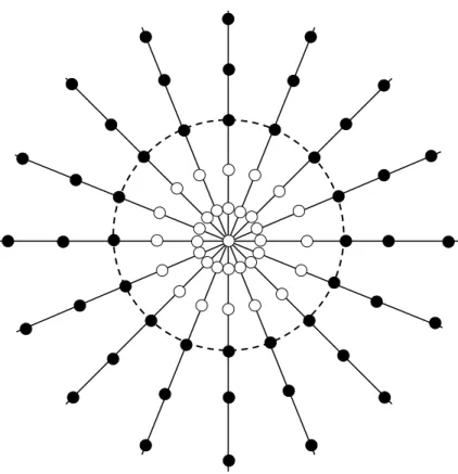
Figure 2.7. The k-space will be adequately covered by the cone surfaces when the separation between individual cones is 1/FOV.
kz
kx
However, the Cones may have drawbacks as well. The increased readout time results to high resolution loss of short-T2 tissues, increased TRs, flow effects as well as off-resonance blurring [21]. Therefore, the length of the spoke or else the readout time of tissues with short-T2 times should not be substantially longer than the T2 of the tissue otherwise the signal will be decayed before the end of the readout.
Zero echo-time (ZTE)
ZTE sequence is a more advanced idea from the UTE. ZTE achieves even shorter TE because it employs a switched-on reading gradient during radiofrequency (RF) excitation [23-26]. ZTE came to prominence once again recently due to the need of imaging lung and bone especially for the PET/MRI. Novel methods of ZTE have been developed [27, 28] and tested already on animals [29] and human skull [30] and lung [31]. ZTE can normally be operated with short TRs and small FA in a magnetization steady state (Fig. 2.10).
Figure 2.8. The resulting gradient waveforms of 3D UTE Cones.
Figure 2.9. Density correction map for all spokes and points. Above: density correction for 3D PR acquisition. Below: density correction for 3D Cones. A zero weighting factor is set for the central k-space while progressively increases along the spoke. For the outermost points there is a drop-off so the high-frequency noise is supressed (apodization).
ZTE uses a nonselective hard pulse excitation while the readout is achieved on a 3D centre-out radial fashion. Main characteristic of the ZTE is that the readout gradients are constantly on and not ramped down something that results in the characteristic short TR that translates to fast scans. Similarly, the image encoding gradients are on when the RF excitation happens, getting the TE down to theoretically 0 where the nominal TE is the centre k-space TE (Fig. 2.11).
Another interesting fact of the sequence is that the data acquisition is grouped into segments with a certain number of spokes so that pre-pulses can be played out for contrast preparation, chemical shift selective saturation or motion navigators. ZTE uses FA of few degrees so the image has inherently PD weighted contrast. Overall the short duration of the RF pulse together with the gradient ramping that is kept to a minimum, lead to a fast and very SNR efficient scanning.
a
a a
a a
a a
RF a Gz
Gx
Gy
Figure 2.10. ZTE pulse sequence. The gradients are kept active during the RF pulsing with only small directional updates in between repetitions, resulting in a nominal TE = 0 as well as fast and quiet scanning. The pulse sequence is grouped into segments (one segment illustrated here) to spoke preparation pulses and/or motion navigators.
However due to hardware constraints, the switching of the transmit/receive gradients off and on requires some time that leads to a delay or dead time between excitation and acquisition. This results to an acquisition gap at the central portion of the k-space (Fig. 2.12).
Reconstruction of UTE sequences
3D Cones belongs to the family of non-cartesian acquisition sequences (Fig. 2.13). The acquired data points of radial, spiral and cones trajectories need first to be projected on a cartesian grid before reconstructing the images.
The algorithm behind it, is called re-gridding (Fig. 2.14). There can be either 2D or 3D re-gridding algorithms which employ the same idea. There is a variety of such algorithms, with the most popular one being the “data driven”
interpolation that takes into account the contribution from each data point and adds it to the adjacent grid points [32-34].
t
t
t
0 delay
G
RF
sample s
Figure 2.11. After the projection gradient G reached full amplitude, a short radiofrequency pulse is emitted and the free induction decay signal is measured as soon as possible (black dots denote acquired data, white dots are missing data).
At the end, re-gridding is just resampling the non-cartesian data onto cartsian plane and then applying inverse Fast Fourier Transform (FFT). After choosing the re-gridding kernel (e.g. Kaiser Bessel function) and applying the density correction factors, the data are convoluted with the kernel and oversampled on the cartesian grid. Then inverse FFT is applied and the image is finally de-apodized. Another idea is also proposed where non-uniform fast Fourier transformation is employed, which is a generalized version of the re- gridding algorithm with forward and inverse implementation which lead to a faster acquisition [35].
Figure 2.12. The 3D ZTE k-space is covered with 1D spoke in a center-out radial fashion white points are non-acquired data, black points represent acquired data.
Figure 2.13. 3D Cones acquisition trajectory (detail on 2D x-y plane). The black dots are the acquired data points, not sampled on a cartesian grid. The distance between the data points depends on the bandwidth of the acquisition. Normally up to 256 kHz can be achieved meaning that the signal is sampled every 4us.
Figure 2.14. Illustration of how the non cartesian data are interpolated onto the cartesian grid using an appropriate kernel (green circle). The data points on the cartesian grid are a weighted sum of all neighboring non-cartesian data.
Chapter III
Optimization of the 3D UTE Cones
You should not desire the impossible Chilon of Lacedaemon
3.1. Introduction
The purpose of this chapter is to give a useful insight on the necessary implemented optimization process of the Cones sequence. Cones is a research sequence which is neither CE marked nor a commercial product. Therefore, various parameters had to be adjusted e.g. programming-wise the sequence needed to be more robust and stable, we needed to investigate which coil configuration is more suitable for our clinical needs & if manual pre-scan is better than auto-scan to avoid overflow artifacts. Additionally, we wanted to make the sequence more time-efficient by avoiding unnecessary time prolongation i.e. longer TR, we enabled prospective triggering using respiration belts worn by the patient and enabled slab excitation using pulses from the GE RF-pulse library. Purpose of the whole optimization was to improve image quality by avoiding artifacts and increasing SNR while shortening scan time which is clinically very important.
3.2. Materials & Methods
The source code of the Cones is provided by GE and is written in a programming language called EPIC (Environment for Pulse programming In C). Cones is a sequence from the General Electric PSD (Pulse Sequence Development) collection. The main prerequisites for the use of the sequence include basic operation of the GE scanner, use of compilers & debugger, familiarity with ANSI C, C++ and basic UNIX commands like makefile, csh, bash.
3.3. Debugging
As first step of the optimization, a general debugging of the code was necessary. First trials to run the sequence led to downloading failures on the scanner, due to compiling errors. The compiling procedure produces the two executable files (one for the host computer - which is the user IO for the image
display & processing, archiving - and one for the target computer, the real- time computer, which controls the looping, the syncing of gradients and the controlling of data acquisition) that need to be saved inside the scanner directory of the sequence. Some of the variables were overlapping and they did not have as default the values that they should, basically some timing variables for delays between consecutive TRs. Another reason was that the software version of the scanner and the compiling environment were not identical. This happens with every software package update of the scanner.
The sequence code needed to be updated to the current PSD package version that runs on the scanner by adding some patches especially on the data acquisition section and how the Specific Absorption Rate (SAR) and other regulatory safety limits are calculated.
3.4. Enabling Prospective triggering
First coding intervention for better lung imaging, concerns the compensation for respiratory lung motion. Lung motion during respiration can induce artifacts and resolution loss. The physiological signal can be acquired by a respiration bellow (Fig. 3.1) that keeps track of the lung’s respiration cycle based on the lung volume increases and decreases through inhalation and exhalation phases. The respiration bellow is worn by the patient around the diaphragm. The triggering point is set to 30% of the maximum expiration and after a delay of 0.1 seconds the data acquisition starts. We add this delay to make sure that the data acquisition will take place as much as possible in the expiration phase. The number of spokes per trigger is fixed to 500. The duration of each spoke corresponds to the duration of each TR. The smaller the number of spokes the better motion correction we get, because the acquisition happens within the end-expiration phase without including motion during exhalation and consequent inhalation, but the scan takes more time. Clinically, even around 50% acquisition window would be acceptable translating into a doubling of the original scan time. However, the 50%
window is a bit large allowing a lot of motion to be detected so a 30% is a good trade off.
3.5. Shortening the TR:
There are three sequence parameters that we manipulated to achieve the overall shortening of the TR.
o Start of Sequence Interrupt (SSI) timing variable o spoiler gradient duration
o rewinder gradient
3.5.1. SSI time
The SSI time is a timing variable specific to EPIC and defined as the interval between the End of Sequence (EOS) and SSI.
EOS are special fields specific in both the waveform and instruction memories, in other terms a memory pointer. When an EOS is encountered in the waveform memory, everything happens as usual until the current duration is over and then the next instruction is used. This also implies that the internal copy of the waveform pointer will be overwritten by the values found in the next instruction. When an EOS is encountered in the instruction memory, the sequence will stop until it is told to start again. EOS monitors the stop and pause flags at the end of the sequence. It Figure 3.1. Respiratory motion (bottom) detected by the respiration bellow worn by the patient on the diaphragm as depicted on the control screen of the scanner.
also handles the re-enabling of the SSI trigger after the new sequence preparations have been updated.
SSI makes realtime changes to the current sequence based on environmental inputs (e.g. patient physiological data) and special algorithms (e.g. Cine) by calling PSD supplied routines at the start of the sequence.
Too long SSI time prolongs unnecessarily the TR, too short SSI time leads to possible crashes since we are using as input the respiratory physiological data and there should be a timing allowance for the psysiological signal to be integrated into the running sequence. The original SSI time was fixed to 500 us and we reduced it to 100 us, without observing any obstacles during the playing out of the sequence.
This translates to 0.4 ms shorter TR.
3.5.2. Spoiler Gradient
The spoiler is applied during gradient echo sequences to remove transverse magnetization by producing a rapid variation of its phase along the direction of the gradient. This takes place after the echo so that the transverse magnetization is destroyed prior to the next excitation pulse to spoil any remaining x-y magnetization. The duration of the spoiler gradient prolongs significantly the acquisition’s TR making the scans longer. However, minimizing or turning the spoiler gradient completely off may present some artifacts concerning the image quality (Fig. 3.2). Because the length of each of the spokes varies based on the desired in-plane resolution and prescribed FOV, the effect of the spoiler’s duration varies as well. For example, for a high resolution scan (e.g. 1.4 mm) the spoke has a length of 250 points. With an acquisition bandwidth (BW) of 250 kHz, this means sampling of k-space happens every 4 us translating to 250 * 4 us = 1000 us or 1 ms which is a bit longer that the T2* (850us) for lung at 3 T. This means that the signal mostly is decayed till the last acquisition point so there is no need for extra spoiling.
Similarly, for a lower resolution scan (e.g. 2mm) with 200 points along each spoke (so 200 * 4 us = 800 us) there is some remaining signal so here turning off the spoiler will affect the image. Thus, there is a trade-off and an optimized spoiler duration for any required resolution. We can skip the spoiler at higher resolutions and we should have it on, with increasing duration for lower- resolution acquisitions. The original spoiler duration was 6000 us and with our desired resolution at 1.4 mm we set the spoiler at 2000 us allowing for a 4000 us (4ms) reduction in TR. The reduction of the spoiler duration has the biggest contribution to the shorterning of the TR.
3.5.3. Rewinder gradient & Flip Angle
The rewinder gradient – in the form of a trapezoid gradient - is another phase- encoding step, that is applied with reverse polarity at the end of every TR.
The role of this gradient is to make sure that the phase of the MR signal is stable in every TR and to assist in the development of coherent transverse magnetization. The effects of not applying a rewinder are resonant offsets that vary from TR to TR, so there can be a contamination of phase-encoded information in consecutive TRs leading to stimulated echoes and rigning bands in the image for non-cartesian acquisitions like Cones.
Figure 3.2. Single channel axial slice image. Left: acquisition with the spoiler gradient turned off. Right image: acquisition with spoiler gradient on.
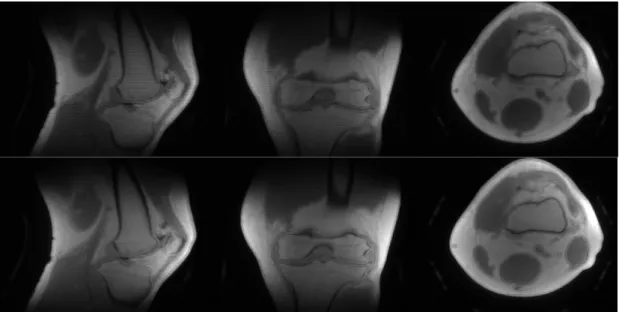
The rewinder has a fixed duration of 700 us. After testing protocols with and without rewinder gradient we optimized our protocol by switching off the rewinder altogether, reducing the TR further by 0.7 ms. Phantom and in-vivo studies (Fig. 3.3, 3.4 & 3.5) show the effects of not using the rewinder (which are more prominent for higher resolution) while for in-vivo studies are stronlgy mediated to negligible.
In addition, for the UTE sequences the FA has a minimal effect. Despite that, based on the Ernst equation, we calculated the optimized FA for maximizing the signal intensity:
𝜃 = cos!"𝑒!(!"!#) [Eq. 3.1]
with TR 3.8 ms and T1 1000 ms for lung tissue the FA is optimum with 5 degrees. The original protocol was using 10 degrees.
Figure 3.3. Upper images: phantom scan without rewinder. Lower images:
phantom scan with rewinder.
3.6. Overflow artifact & Receiver Coil Gain
The overflow artifact appears due to prescan malcalibration and causes a non- uniform washed out appearance to the images. The high intensity signal after excitation due to ultra-short TEs (28 us), overflows the dynamic range of the receiver channel leading to the clipping and inversion of pixel bits. The cause of this, is that the signal is too intense and cannot be accurately digitized by the analog-to-digital (ADC) converter.
Figure 3.4. Upper images: knee scan without rewinder. Lower images: knee scan with rewinder.
Figure 3.5. Axial slice of a 2mm in-plane resolution with (left) and without (right) rewinder gradient. Effects are quite minimal if non-existent with a significant reduction in scan time.
To overcome this, the receiver gains R1 and R2 have to be adjusted manually (manual prescan). Lowering the R1 and R2 theoretically affects also the sensitivity to the real signal but the images still looked good with a small reduction of the gain values. One way to deter this artifact is by the auto- prescanning but sometimes this fails to compensate for this effect, so another way is to manually decrease the receiver gain. An alternative, to avoid this artifact, is by positioning the patient with arms up during the scan because the signal is very high from soft tissues like the muscles on the arms.
Some clinical examples are presented in this section. Fig. 3.6 and 3.7 show an axial slice of a lung scan with full coil gain based on prescan autocalibration (left) and after adjusting the R1 and R2 receiver gains by manual prescan (right). The figures show two different groups of selected individual channels.
In Fig. 3.6. (left) there are dominant overflowing artifacts contaminating the entirety of the slice. Note that the signal from the lungs is white and from muscles black. On the right of the same figure, the contrast has been recovered with the exception of some outside FOV artifacts that anyway are irrelevant to the receiver gain. Another important detail that shows the improvement can be seen in Fig. 3.7. On the right, an axial slice, after the automatic prescan, with noisy trachea and noisy background.
Figure 3.6. Overflow artifact with full coil gain (left) & avoiding artifact with reduced coil gain (right).
The background and trachea appear darker on the left, after manual prescan with lower R1 & R2 values, with a clearly lower noise level, while also the signal from the lung parenchyma appears higher.
It is interesting also to look at what happens on the background, in the signal itself, by looking at the profile of the spokes of cones from saturated channels.
In Fig. 3.8. one can see the DC (central k-space point) signal profile of the spokes for the same channel under manual calibration (upper) and under overflowing artifact conditions (lower). Except for the amplitude of the signal, which is significantly lower for the overflown channel, after the so-called clipping takes place, the digitization failure is apparent. The sharp regional peaks in both upper and lower diagrams exist because the acquisition is respiratory triggered showing that the acquisition starts during mid- exhalation (higher amplitude) till it reaches full end-expiration (lower signal plateau). In Fig. 3.9. one can see the profile of one spoke for all data points from DC to the last point of the trajectory. Similarly, on the left, the profile of the spoke with normal dynamic range shows high amplitude and a smooth profile. Opposite, on the right diagram, the same spoke under overflown effects where the amplitude is cropped and without a distinctive decaying profile of the FID signal.
Figure 3.7. Full coil gain (R1 & R2) axial image (left) and with reduced gain (right), noisy trachea compared to black trachea. In addition, the background is much smoother than the background in the full gain acquisition.
Figure 3.8. Upper image: DC signal from the channel near the diaphragm. The respiratory gating is evident from the sharp change from low to maximum signal.
Lower image: DC signal from the same channel that is overflown. The intensity of the signal is much less (clipped) and the digitization failure is evident.
Figure 3.9. One spoke-intensity profile from center (0 point) out (200th point). Left image: normal dynamic range. Right image: channel with overflow artifact.
0 50 100 150 200 10000
8000
6000
4000
2000
900 800 700 600 500 400 300 200 100
0 50 100 150 200
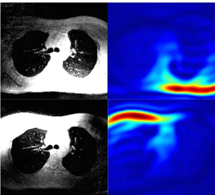
Fig. 3.10. presents an illustrative detailed diagram of one spoke for all points along its trajectory. The real time-dependent magnitude of the amplitude is shown on the upper part while on the lower part one can see how the digitization of the FID from ADC fails when there is signal cut off from too large analog FID. Based on the coil configuration and the spatial sensitivity of the receiver channels, the clipping comes with various amplitude-level changes so the effects on the image quality are varying from prominent to mild. A couple of examples are shown in Fig. 3.11. and 3.12. Fig. 3.11 shows axial slices with their sensitivity profiles of a single channel with overflown artifact and inversed dynamic range. The sensitivity profile in both cases is not homogeneous and there is an increased sensitivity in the nearest body region. In contrast, Fig. 3.12 shows two single-channels, one posterior and one anterior of the same axial slice of a normal dynamic range scan. The corresponding sensitivities here are homogeneous and well-contained.
Figure 3.10. RF Overflow artifact (detail).The ADC fails to accommodate the whole signal leading to clipping and digitization failure. This leads to the characteristic washed-out effect on the images.
analog FID from RF coil
time
induced voltage
signal cut off from too large analog FID
digitized FID from ADC
Figure 3.12. Two individual channel images and corresponding sensitivity profiles of the same slice. Upper: posterior single channel selection, lower: anterior single channel selection.
Figure 3.11. RF overflow artifact examples of different axial slices with their corresponding channel sensitivity profiles.
50 100 150 200 250
50
100
150
200
250
3.7. Spoke length and acquisition time
It is already stated that the more twisting we add to the spokes of the Cones, the less cones we need to cover the k-space, so a reduction in scan time is achieved. However, the TR is prolonged since more data points are added to each duty cycle. With how much twisting one can go depends mainly on the required resolution and is limited by the T2* since we do not want to keep acquiring data points much further from the point that the signal has already decayed. Fig. 3.13 shows the effect of different spoke lengths under no-spoiler gradient condition. An axial slice with 220 points (left) and 280 points (right) along the spokes is shown. While the acquisition with 220 points corresponds to 880 us which is shortly after T2*, there is some transverse magnetization left and this affects the image with the ringing artifacts. While with 280 points that correspond to 1120 us, the remaining magnetization has completely decayed and the image quality is recovered. Even if we use a spoiler gradient and we select a too long spoke length the effect on the image will be the same as in the left image of the Fig. 3.13, but there the reason is that the k-space is filling with too many high frequency noise points.
Figure 3.13. Axial slice of a 2mm in-plane resolution scan with selected posterior channels. Images with 220 points per spoke (left) versus 280 points per spoke (right) with rewinder and spoiler gradients off. The longer trajectory compensates for the absence of the spoiler and allows the tranverse magnetization to sufficiently decay before next TR.
3.8. Slab excitation pulse
For our protocol, we enabled also a slab selective minimum phase Shinnar- Le Roux (SLR) pulse. The nominal pulse width was set to 1128 us, the RF pulse spectral bandwidth to 16 kHz with an absolute width of 0.14 us and an effective width 0.0686 us. This was the first time to use slab excitation with Cones so we could minimize outside-of-FOV artifacts across the main perpendicular plane. For example, if the scan is acquired on the axial plane, then the RF slab excitation pulse can hinder acquiring signal from outside the coronal FOV (neck and abdomen). Furthermore one can adjust how much of the FOV the acquisition can cover so for example with a slab-strecthing factor of more than 1.0 we can acquire also body regions extending further from the FOV or if the factor is lower than 1.0 we can see dark bands (signal loss) on the upper and lower parts of the image whose extension is proportional to the prescribed factor.
3.9. Calibration Scan of Cones
For a well performing Cones, a calibration scan needs to be run once, after the installation of the sequence so gradient delays can be adjusted. Purpose of this calibration scan is to start the acquisition from the center of k-space otherwise there is a halo effect around the imaging object. Practically, is an offset correction of the sequence. Time delay between gradient kick on and acquisition is set to 2 us since this gives the best performance and stability to the sequence.
3.10. Putting optimized Cones to the test
After all these optimization steps, Cones was tested on volunteers and clinically. In this paragraph some of the initial testing scans will be depicted.
The protocol that was used had the following parameters: 1.4 mm in plane resolution, 4 mm slice thickness, TE 0.028 us, TR 3.8 ms, FA 5 degrees, spokes per trigger 500, no rewinder gradient, spoiler duration 2000 us and scan time of 3:40 minutes. Fig. 3.14. shows high resolution examples of lung diagnostic scans of cones with very good respiratory motion correction and very good depiction of structures like vessels and airways inside the lungs in both axial slices and maximum intensity projections (MIPs).
Figure 3.14. Upper images: axial single slices and MIPs of the axial, sagittal and coronal planes of the scan acquired with 1.4 mm in plane resolution and 4 mm slice thickness. Lower images: similarly, the images here from the scan with isotropic resolution of 1.4 mm.
Apart for the lungs, the Cones were tested also for bone imaging with a knee scan. In Fig. 3.15 the bone anatomy of the knee (femur, patella, tibia) is well depicted with Cones. For bone imaging, we tested knee under-sampled acquisitions reconstructed with the CG-SENSE method (see Chapter VI) as well (Fig. 3.16).
Figure 3.15. Knee images with 3D UTE Cones with 1.4 mm isotropic resolution.
Figure 3.16. Upper and lower images show two different axial slices of the knee.
Left images show the original fully sampled images, the medium ones show the 50%
under-sampled acquisitions with heavy artifacts and the right images show the recovered images with the CG-SENSE reconstruction after 10 iterations that yielded the best results.
After testing, the best coil configuration is thought to be as small as possible so we can cover the FOV that is prescribed as tight as possible to the lungs with the fewest possible combination of channels. Otherwise the additional unnecessary channels can induce outside of FOV artifacts in the image as depicted in Fig. 3.17.
Finally, a clinical comparison between Cones, PROPELLER and LAVA-Flex of a patient with double pleural effusion (Fig. 3.18) and neighbouring inflammation. While PROPELLER provides excellent contrast for the fluid depiction, it fails to deliver as much when it comes to the inflammation on top. LAVA-Flex similarly has not as much contrast as Cones while both PROPELLER and Lava-Flex do not capture lung parenchyma which is visible in Cones (higher contrast between lung signal and background). As far as the scan time is concerned, Cones came with 3:50 minutes, PROPELLER with 6 minutes and LAVA-Flex with a breathold of 20 seconds.
50 100 150 200 250 300
50
100
150
200
250
300
Figure 3.17. Outside of FOV artifact. Smaller coil configuration solves the issue.
Figure 3.18. An axial slice of a patient with double pleural effusion and inflammation on both lungs scanned with Cones (left), PROPELLER (center) and LAVA-Flex (right).
Cones was tested also on pediatric cases. Here some images are presented in Figure 3.19 with healthy lungs in all three tomographical planes while in Figure 3.20 scans of lung pathology with cystic fibrosis are shown. For comparison, PROPELLER images are also shown.
Figure 3.19. 3D UTE Cones of pediatric patient with healthy lungs on axial, coronal and sagittal slices (left) and Maximum Intensity Projection (right) with PROPELLER for comparison.
Figure 3.20. 3D UTE Cones (upper) and PROPELLER (lower) axial slices of pediatric patients with cystic fibroris. Cystic fibrosis with air- trapping and mucus plugging were among the common diagnosis.
Figure 3.20. 3D UTE Cones (upper) and PROPELLER (lower) axial slices of pediatric patients with cystic fibroris. Cystic fibrosis with air- trapping and mucus plugging were among the common diagnosis.
Figure 3.20. 3D UTE Cones (upper) and PROPELLER (lower) axial slices of pediatric patients with cystic fibroris.
Cystic fibrosis with air-trapping and mucus plugging were among the common diagnosis.