extension to OLCI data

(1)

extension to OLCI data

Hongyan Xi

^a,⁎

, Svetlana N. Losa

^a,b

, Antoine Mangin

^c

, Mariana A. Soppa

^a

, Philippe Garnesson

^c

, Julien Demaria

^c

, Yangyang Liu

^a,d

, Odile Hembise Fanton d'Andon

^c

, Astrid Bracher

^a,e

aAlfred Wegener Institute, Helmholtz Centre for Polar and Marine Research, Bremerhaven, Germany

bShirshov Institute of Oceanology, Russian Academy of Sciences, Moscow, Russia

cACRI-ST, 06904 Sophia Antipolis Cedex, France

dFaculty of Biology and Chemistry, University of Bremen, Bremen, Germany

eInstitute of Environmental Physics, University of Bremen, Bremen, Germany

A R T I C L E I N F O Edited by Menghua Wang Keywords:

Retrieval algorithm Chlorophylla

Phytoplankton functional types Empirical orthogonal functions Remote sensing reflectance HPLC pigments CMEMS GlobColour OLCI

A B S T R A C T

This study presents an algorithm for globally retrieving chlorophylla(Chl-a) concentrations of phytoplankton functional types (PFTs) from multi-sensor merged ocean color (OC) products or Sentinel-3A (S3) Ocean and Land Color Instrument (OLCI) data from the GlobColour archive in the frame of the Copernicus Marine Environmental Monitoring Service (CMEMS). The retrieved PFTs include diatoms, haptophytes, dinoflagellates, green algae and prokaryotic phytoplankton. A previously proposed method to retrieve various phytoplankton pigments, based on empirical orthogonal functions (EOF), is investigated and adapted to retrieve Chl-a concentrations of multiple PFTs using extensive global data sets of in situ pigment measurements and matchups with satellite OC products.

The performance of the EOF-based approach is assessed and cross-validated statistically. The retrieved PFTs are compared with those derived from diagnostic pigment analysis (DPA) based on in situ pigment measurements.

Results show that the approach predicts well Chl-aconcentrations of most of the mentioned PFTs. The performance of the approach is, however, less accurate for prokaryotes, possibly due to their general low variability and small concentration range resulting in a weak signal which is extracted from the reflectance data and corresponding EOF modes. As a demonstration of the approach utilization, the EOF-based fitted models based on satellite reflectance products at nine bands are applied to the monthly GlobColour merged products.

Climatological characteristics of the PFTs are also evaluated based on ten years of merged products (2002−2012) through inter-comparisons with other existing satellite derived products on phytoplankton composition including phytoplankton size class (PSC), SynSenPFT, OC-PFT and PHYSAT. Inter-comparisons indicate that most PFTs retrieved by our study agree well with previous corresponding PFT/PSC products, except that prokaryotes show higher Chl-aconcentration in low latitudes. PFT dominance derived from our products is in general well consistent with the PHYSAT product. A preliminary experiment of the retrieval algorithm using eleven OLCI bands is applied to monthly OLCI products, showing comparable PFT distributions with those from the merged products, though the matchup data for OLCI are limited both in number and coverage. This study is to ultimately deliver satellite global PFT products for long-term continuous observation, which will be updated timely with upcoming OC data, for a comprehensive understanding of the variability of phytoplankton composition structure at a global or regional scale.

1. Introduction

Over the past decades, satellite ocean color (OC) remote sensing has been widely used for estimating chlorophylla (Chl-a) concentration, which is often used as an indicator of phytoplankton biomass. Beyond

that, extracting information on phytoplankton community structure, e.g., phytoplankton functional types (PFTs), size classes (PSCs) and taxonomic composition, has become a research topic of priority, as it plays an important role in understanding the marine food web and aids the modelling associated with climate change impacts on

https://doi.org/10.1016/j.rse.2020.111704

Received 4 July 2019; Received in revised form 7 January 2020; Accepted 3 February 2020

⁎Corresponding author.

E-mail address:Hongyan.Xi@awi.de(H. Xi).

(2)

biogeochemical and ecological cycling of oceans (e.g.,Falkowski et al., 1998;Le Quéré et al., 2005;IPCC, 2013;Bracher et al., 2017). In addition, accurate estimation on phytoplankton diversity and group distribution provides valuable information on identifying blooms caused by specific toxic algae, i.e., harmful algal blooms such as cyanobacterial blooms and red tides (e.g.,Craig et al., 2006;Hu et al., 2010;Wang et al., 2017). A PFT is usually defined as a homologous set of "organisms related through common biogeochemical processes" such as silicifica- tion, calcification, nitrogen fixation, or dimethyl sulfide production, but are not necessarily phylogenetically affiliated (Falkowski et al., 2003;

Litchman et al., 2006;IOCCG, 2014). However, as many phytoplankton groups which can be detected by remote sensing are also functional types, (e.g., diatoms are silicifiers, some cyanobacteria are nitrogen fixers, and coccolithophorids are calcifiers) (Bracher et al., 2017), these satellite proxies have been named PFTs for brevity (e.g., Losa et al., 2017).

Satellite OC remote sensing enables observation of phytoplankton over large areas or even at global scale. With previous (e.g., Sea- Viewing Wide Field-of-View Sensor – SeaWiFS and MEdium Resolution Imaging Spectrometer – MERIS) and current available OC satellites Moderate Resolution Imaging Spectroradiometer (MODIS), Visible Infrared Imaging Radiometer Suite (VIIRS), and especially the newly launched OLCI onboard Sentinel-3A (in February 2016) and 3B (in April 2018), a vast amount of quality controlled OC data are collected, allowing us to contribute to developing and/or improving methods and the corresponding applications to satellite data for estimating biogeochemical parameters in terms of global observation. There is a clear need to implement a sound PFT retrieval algorithm to the recent OLCI data, as well as to previous and current satellite OC time series data such as CMEMS GlobColour merged products (ACRI-ST GlobColour Team et al., 2017).

Different bio-optical and ecological algorithms have been developed to identify PFTs and phytoplankton taxonomic composition at the ocean surface, mainly based on phytoplankton abundance and in- herent/apparent optical properties. Abundance-based approaches seek to establish empirical relationships between the PFTs and phytoplankton abundance or biomass, such as Chl-aconcentration that can be retrieved from satellites (e.g.,Uitz et al., 2006;Brewin et al., 2010, 2015; Hirata et al., 2011). Ecological-based approaches incorporate additional environmental parameters to identify ecological niches where particular phytoplankton communities may be found (Raitsos et al., 2008;Palacz et al., 2013). Efforts have also been made to com- bine abundance and ecological-based approaches (e.g. Brewin et al., 2015;Ward, 2015). Spectral-based approaches are more direct as they target known optical signatures and use satellite observed spectra to extract the signatures of specific PFT (e.g.,Ciotti and Bricaud, 2006;

Devred et al., 2006; Alvain et al., 2005, 2008; Hirata et al., 2008;

Bracher et al., 2009; Kostadinov et al., 2009; Werdell et al., 2014;

Brewin et al., 2015;Correa-Ramirez et al., 2018). These methods are mainly based on radiative transfer or bio-optical models and generally require high computation performance and adaptations for specific sensors. More complete reviews of these approaches are well detailed by the works of theIOCCG (2014),Bracher et al. (2017), andMouw et al. (2017).

In this study, we seek to establish an approach that uses satellite reflectance data which inherit the information of various phytoplankton pigments and, therefore, allows retrieving the Chl-a concentrations of multiple PFTs. We choose the empirical orthogonal function (EOF) analysis, also known as principal component analysis, as it has been previously used for predicting ocean color metrics and various phytoplankton pigment concentrations by assessing variance of structures in spectral remote sensing reflectance (Rrs) or water leaving radiance (e.g.,Lubac and Loisel, 2007;Craig et al., 2012;Taylor et al., 2013;Bracher et al., 2015;Soja-Woźniak et al., 2017). The spectral data are subject to EOF analysis to reduce the high dimensionality of the data and derive the dominant signals (EOF modes) that best describe

the variance within the data set. Studies also proved that the EOF analysis could provide reliable retrievals even with limited number of data points (Craig et al., 2012;Bracher et al., 2015). Another advantage is that the models exhibited negligible loss of skill when applied to data sets with a reduced spectral resolution, which enables the applicability to the previous or currently existing multispectral OC sensors and future hyperspectral satellite missions such as PACE (Gregg and Rousseaux, 2017), HyspIRI (Lee et al., 2015) and EnMAP (Guanter et al., 2015).

Given that the EOFs derived from in situ or satellite hyper-/multispectral R_rsdata have provided reliable retrievals of the concentrations of Chl-aand different pigments/pigment groups (Taylor et al., 2013;

Bracher et al., 2015), we intend to present an implementation of the method proposed inBracher et al. (2015)to retrieve PFTs instead of pigments, and to up-scale the application from regional to global scale by constructing large in situ data sets and multi-sensor OC products.

Therefore, with the use of extensive in situ phytoplankton pigment data sets, satellite OC products, and matchups between in situ and satellite data, we propose an EOF-based global PFT retrieval approach by linking the variances in Rrsspectral structures to different PFTs. In the present study, we aim firstly to establish the EOF fitted model based on the nearly globally covered matchups between the satellite Rrsand the PFT Chl-a concentrations derived from diagnostic pigment analysis (DPA) of in situ HPLC pigment data, and cross-validate the performance of the EOF-based algorithm statistically; secondly, to set up the PFT retrieval scheme based on the EOF modes obtained from the matchups for the implementation to satellite OC products; thirdly, to investigate and evaluate the climatological characteristics of the PFTs retrieved from merged OC products (2002–2012) through inter-comparisons with other existing PFT/PSC products at the same period, and finally, to explore the potential of applying the approach to OLCI products based on a prediction scheme using a much more limited number of matchups.

2. Data and methods 2.1. Data sets

2.1.1. In situ databases of phytoplankton pigments

2.1.1.1. Pigment Database I (1997–2012). A large data set of the quality controlled near surface (first 12 m) HPLC phytoplankton pigments built for the ESA SynSenPFT Project (Bracher et al., 2016) was used for the extraction of the collocated R_rsspectra from satellite data. This HPLC pigment data set includes >15,000 sets of phytoplankton pigment data spanning 25 years from 1988 to 2012 covering the global ocean, collected from SEABASS, MAREDAT, LTER, BATS, AESOP-CSIRO, LOV and also from our own data published at PANGAEA (see Table 1 inLosa et al., 2017). Since SeaWiFS as an earlier OC sensor was launched in 1997, a subset for the period of 1997–2012 including 11,977 sets of pigment data was taken as Pigment Database I and used for the extraction of the Rrs matchups from GlobColour merged products.

Yearly coverage of this matchup database spans from 3.2% (the least data points for 2012) to 9.3% (the most for 2004). 24.1%, 17.4%, 21.1%, and 37.4% of the data were collected during March–May, June–August, September–November, and December–February, respectively.Fig. 1(A) shows the spatial distribution of all the data points in this database in which all pigments are included, but only total chlorophyllaconcentration (TChl-a, sum of monovinyl chlorophylla, divinyl chlorophylla, chlorophyll aallomers, chlorophyll a epimers, and chlorophyllidea) is present in the figure.

2.1.1.2. Pigment Database II (2016–2018). A relatively smaller (n= 992) phytoplankton pigment database of quality controlled near surface HPLC pigments was also built for the OLCI matchups from 2016 to 2018, involving our recently published data sets of HPLC based phytoplankton pigment concentrations collected mainly in late spring and summer from five cruises – Heincke462 in the North Sea

(3)

(April–May 2016):https://doi.pangaea.de/10.1594/PANGAEA.899043 (Bracher and Wiegmann, 2019), PS99 in the North Sea and the Fram Strait Arctic (June–July 2016): https://doi.pangaea.de/10.1594/

PANGAEA.905502 (PS99.1) and https://doi.pangaea.de/10.1594/

PANGAEA.898102(PS99.2) (Liu et al., 2019a, 2019c), PS103 in the Southern Ocean: https://doi.pangaea.de/10.1594/PANGAEA.898941 (Bracher, 2019) (December 2016–January 2017), PS107 in the Fram Strait Arctic (July–August 2017): https://doi.pangaea.de/10.1594/

PANGAEA.898100(Liu et al., 2019b), and PS113 in the trans-Atlantic Ocean (May–June 2018): https://doi.pangaea.de/10.1594/PANGAEA.

911061(Bracher et al., 2020).Fig. 1(B) shows the locations of the data

points from Pigment Database II (including all the pigments but with only TChl-aconcentration present in the figure), which covers a large range of latitudes but focuses on the Atlantic Ocean only (60°W–20°E).

2.1.2. Satellite ocean color data

Satellite normalized remote sensing reflectance (Rrs) Level-3 (L3) products from multiple sensors were obtained from the CMEMS GlobColour data archive (http://www.globcolour.info/). The Rrspro- ducts used for matchup analysis included daily R_rsL3 products with 4- km resolution at the bands from either individual sensors (SeaWiFS, MODIS, MERIS, and VIIRS onboard Suomi-NPP) or the merged products

Fig. 1.Spatial distribution of the TChl-aconcentration from the quality controlled in situ (A) Pigment Database I (1997–2012), and (B) Pigment Database II (2016–2018).

(4)

of two or more sensors. More details on the merged products are given in the GlobColour Product User Guide (ACRI-ST GlobColour Team et al., 2017). Rrsproducts from OLCI were not merged with any other sensor products and were therefore used separately for an OLCI only PFT retrieval scheme. Similar to the merged products, daily 4 km RrsL3 products of OLCI were used for matchup extraction. In further application of the proposed approach to derive global long time series PFT products, monthly RrsL3 products with 25 km spatial resolution from both, the merged products and OLCI data, were obtained for July 2002–April 2012 (time when SeaWiFS, MODIS and MERIS were in orbit, although SeaWiFS operation ended in late 2010 and then in late 2011 VIIRS was added), and April 2016–December 2018 (OLCI on Sentinel-3A in operation), respectively. In addition, the GlobColour merged ocean TChl-amonthly products with 25 km resolution in July 2002–April 2012 were also obtained for inter-comparison. The merged L3 TChl-aproducts were derived by a weighted average method (AVW) from single-sensor Level 2 chlorophyll products for case 1 waters (ACRI-ST GlobColour Team et al., 2017).

2.1.3. PFT retrieval input data

(A) PFT Chl-aconcentrations derived from diagnostic pigment analysis (DPA)

Chl-aconcentrations of PFTs were derived using an updated DPA method (Soppa et al., 2014;Losa et al., 2017). The DPA method was originally developed by Vidussi et al., 2001, adapted in Uitz et al.

(2006)and further refined by Hirata et al. (2011)andBrewin et al.

(2015). Basically, it relates the weighted sum of seven DPs (re- presentative of individual PFTs) to TChl-aconcentration, enabling us to determine the fraction of each PFT to the TChl-athus to derive the PFT Chl-a concentrations. The partial coefficients of the DPs used in this study were derived from multiple linear regression using the data from the large global pigment data set as detailed in Table S1 of Supple- mentary Material inLosa et al. (2017)and were in good agreement with previous studies. The pigment concentrations of fucoxanthin, peridinin, 19′hexanoyloxy-fucoxanthin, 19′butanoyloxy-fucoxanthin, alloxanthin, chlorophyllb, zeaxanthin and divinyl chlorophyllawere used to derive the Chl-aconcentrations of six PFTs in our study, that are, respectively, diatoms and dinoflagellates which are commonly considered as microphytoplankton, two types of nanophytoplankton – haptophytes and green algae (chlorophytes), and two picophytoplankton – prokaryotes, and Prochlorococcus which is a typical species of prokaryotes and commonly found in the subtropical region. PFT Chl-aconcentrations

<0.005 mg m⁻³were excluded as such low values might contain much uncertainty. The rational for this threshold is that the surface Chl-a concentration encountered in the clearest ocean waters (South Pacific Gyre) was found to be in the range 0.01–0.02 mg m⁻³(Morel et al., 2007). Therefore, values below 0.01 mg m⁻³may be questionable. The corresponding PFT Chl-aconcentration can be smaller. Considering the quality control on a large pigment data set as inAiken et al. (2009), we chose the threshold of 0.005 mg m⁻³for PFT Chl-ato minimize the influence of low accuracy in observations on the retrieval model, as it could bring much higher uncertainty to final prediction. The DPA derived PFT Chl-aconcentrations for diatoms, haptophytes and prokaryotes from the pigment database I were published already inLosa et al.

(2017)and are available from PANGAEA:https://doi.pangaea.de/10.

1594/PANGAEA.875879(Soppa et al., 2017).

(B) Matchups between in situ PFT and satellite Rrsdata

Matchups to in situ PFT data were extracted from GlobColour global 4-km daily products for both merged and OLCI products. GlobColour

"L3b" products with a sinusoidal projection were used so that each extracted pixel covers the same area. For each in situ measurement covered by a product, a matchup of 1 × 1 and 3 × 3 pixels around the

in situ location was extracted. No specific quality filtering was applied at this stage because L3 products already exclude bad quality Level-2 pixels (ACRI-ST GlobColour Team et al., 2017). Averaged data based on 3 × 3 pixels were computed using the standard MERMAID tools (http://mermaid.acri.fr/) which follows the protocol fromBailey and Werdell (2006), in summary:

•

only matchups containing at least 50% of valid pixels were kept;

•

outlier pixels with (pixel value – median value) greater than

±1.5∗standard deviation were removed;

•

the matchups were removed if the coefficient of variation (CV) of the remaining pixels was higher than 0.15.

The same extraction and averaging protocol was used for merged and OLCI matchups. Based on the two HPLC pigment databases inSect.

2.1.1, we have obtained the following matchups:

1) Matchups between daily merged Rrs products and in situ PFT data:

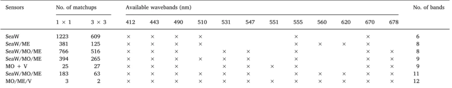
the Rrsspectra at multispectral bands collocated with the PFT data derived from the Pigment Database I inSect. 2.1.1were extracted from the merged products (including SeaWiFS, MODIS, MERIS, VIIRS) from 1997 to 2012 archived in the GlobColour database. The extracted Rrsmatchups included 1 × 1 pixel, and averaged Rrsby 3 × 3 pixels with the median and the standard deviation for each matchup. However, the same wavebands for Rrsdata are not always available because different sensors have different spectral coverage at different periods (in addition to the exclusion of data with bad quality).Table 1lists the numbers of matchups with different band combinations (from six to twelve bands) for R_rs matchups with 1 × 1 pixel and 3 × 3 pixels, respectively.Fig. 2shows the corresponding geographical locations of 1 × 1 pixel matchups for Rrsat eight, nine and eleven bands, where the matchups were to some extent still globally distributed.

2) Matchups between daily OLCI Rrsand in situ PFT data: the Pigment Database II inSect. 2.1.1was used to derive the in situ PFT data and extract the corresponding OLCI Rrsmatchups from 2016 to 2018.

Table 2lists the numbers of matchups with 10, 11 and 12 wavebands for Rrsdata from S3A OLCI with 1 × 1 pixel and 3 × 3 pixels, respectively. Note that OLCI also includes the 709 nm and that OLCI itself does not have a band at 555 nm, but GlobColour database provides for MERIS and OLCI sensors the 555 nm through an inter- spectral conversion using:

Rrs(555) = Rrs(560) ∗ (1.02542–0.03757 ∗ y − 0.00171 ∗ y² + 0.0035∗y³+ 0.00057∗y⁴), where y = log10(CHL1) and CHL1 is the TChl-a concentration estimated by OC4 algorithm (ACRI-ST GlobColour Team et al., 2017). With this conversion, Rrsat 555 nm for OLCI were also included in our study.

2.2. Empirical orthogonal functions (EOF) based algorithm for PFT retrieval 2.2.1. EOF-based statistical approach

Following Bracher et al. (2015), each Rrs spectrum was firstly standardized by subtracting the mean spectral value and then divided by the spectral standard deviation (Taylor et al., 2013). The standardized data set of Rrs, denoted as matrix X (Mobservations ×Nwave- lengths), was collocated to the respective DPA-based PFT data set C withMobservations and 6 PFTs (Mmight be different for the six PFTs).

As indicated in the model training box ofFig. 3, singular value de- composition (SVD) was applied to X for deriving the EOF modes:

=

X U V ,^T (1)

where matrix U (M×N) contains column vectors of scores associated with EOF modes, matrix V (N×N) contains the EOF loadings (spectral pattern), andΛis an N × N matrix containing the singular values of X on the diagonal in decreasing order. For the PFT Chl-a prediction,

(5)

generalized linear models (GLM) were created expressing the log- transformed Chl-aconcentrations of each PFT,C_p, as a function of a subset of EOF scores (U). EOF modes with standard deviations (singular values fromΛ) that are <0.0001 times the standard deviation of the first EOF mode were considered insignificant and thus omitted. The regression model for PFT prediction was expressed as:

= + + + …

C a a u a u a u

ln( )_p ₀ _{1 1} _{2 2} _{n n}, (2)

whereu1,2,…nare the leadingnEOFs from column vectors of U,a0is the intercept and a1,2,…n are the regression coefficients. In addition, a stepwise routine was applied to search for smaller regression models, i.e., lessuvariables, through minimization of the Akaike information criterion (AIC). The significance of included terms was defined by the change in AIC (ΔAIC) with each term's removal.

2.2.2. Model assessment

We consider the coefficient of determination (R²), the slope (S) and the intercept (a) of the GLM regression, which are based on the log- scaled predicted (ln(C_p)) against the log-scaled observed (ln(C_o)) PFT Chl-a concentration data, while the root-mean-square difference (RMSD), the median percent difference (MDPD), and the bias are based on the non-log-transformed data. Model performance statistics are expressed as:

= ⁼

=

C C

R (ln( ) ln( ))

(ln( ) ln( )) ,

i

M pi oi

i

M oi oi

2 1 2

1 2 (3)

= ⁼ C C

RMSD ( M )

i ,

M1 pi oi 2

(4)

= C C × = …

C i

MDPD Median of |( )|

100 , 1, M,

pi oi

oi (5)

= M =

C C

bias 100 ( C )

,

i

M pi oi

1 oi (6)

whereMis the number of observations inCo, andCoiis the mean of the observations, i.e.,Coi =M iM₌ C

1 oi

1 .

To test the robustness of the fitted model, cross-validation of the model fitting was carried out, similar to the procedure performed in Bracher et al. (2015). The collocated data were randomly split into two subsets, in which 80% of the data was used for model fitting/training, which included X^train(standardized Rrsspectra) andC^train(PFT Chl-a concentrations), and the rest 20% was used for prediction validation including X^valandC^val. The procedure was run for 500 permutations to eliminate the model uncertainty produced based on a spatially or temporally biased data set. For each permutation, with Eqs.(1)–(2)and the stepwise routine, a regression model was fitted between ln(C^train) and U^train. The standardized validation set X^valwas then projected onto the EOF loadings V^trainand the inverse of singular valuesΛ^train−1to derive their EOF scores U^val:

=

U^val X^val V^train ^{train 1} (7)

Fig. 2.Geographical locations of the single pixel matchups for merged Rrsat eight (in ×), nine (in△) and eleven bands (in +). (For interpretation of the references to color in this figure legend, the reader is referred to the web version of this article.)

Table 2

Numbers of available OLCI Rrsmatchups with 10, 11 and 12 wavebands.

Number of OLCI matchups OLCI central bands (nm) No. of bands

1 × 1 3 × 3 3 × 3 all^a 400 412 443 490 510 555 560 620 665 674 681 709

115 33 924 × × × × × × × × × × 10

115 33 924 × × × × × × × × × × × 11

86 25 749 × × × × × × × × × × × × 12

a 3 × 3 all: all available pixels in the 3 × 3 square were selected, but only matchup data with more than five out of nine pixels available were used.

(6)

Lastly, the PFT Chl-a concentrations for the validation data set (Cpval) were predicted using U^val of the selected EOF modes and the corresponding regression coefficients. The pairs of the observed and predicted PFT concentrations (CovalandCpval) of the 500 permutations were recorded for model assessment.

For each permutation, the R²for cross validation based on ln(Cpval) versus ln(Coval) is determined, and the mean value of the R²from all permutations (R²cv) is calculated. Similarly, other statistical parameters for cross validation are determined as follows by taking the mean values of the parameters from all permutations:

= ⁼

=

cv c c

c c

R (ln( ) ln( ))

(ln( ) ln( ))

i

M pival

oival i

M oival

oival

2 1 2

1 2 (8)

= ⁼ C C RMSDcv _i^M₁( _pi^valM _oi^val)²

(9)

= ×

= …

C C

C M

MDPDcv Median of |( )|

100 , i 1, (number of points for validation)

pival oival pival

(10)

2.2.3. PFT predictions from satellite data

As illustrated inFig. 3 (model application part), we were able to apply the EOF analysis to satellite R_rs data listed inSect. 2.1.2. Fol- lowing Bracher et al. (2015), to predict PFTs globally using Rrsdata

from merged OC or OLCI products, for which we do not have corresponding pigment and PFT measurements, we projected standardized Rrsdata from the satellite onto the EOF loadings (V) to derive a new set of EOF scores (U^sat), which was subsequently used for the prediction with the fitted model (see equations in model application ofFig. 3), where a0 and a1,2,…n were taken from the model developed with matchups from merged products or OLCI data as listed inSect. 2.1.2.

2.3. PFT relative dominance

With the six retrieved PFTs in our study, we classified the relative PFT dominance in terms of Chl-aconcentration on a global scale. The classification was performed simply based on the absolute values of the retrieved PFT Chl-aconcentrations. For each set of the monthly PFT products, two steps were performed as follows. Step 1: the five PFTs – diatoms, dinoflagellates, haptophytes, green algae and prokaryotes – were compared pixelwise and the one with the highest Chl-a concentration was considered as the dominant PFT at this particular pixel.

Since prokaryotes mainly containProchlorococcusandSynechococcus- like-cyanobacteria (SLC), Step 2 was performed to further assign the dominance of prokaryotes to eitherProchlorococcus-dominated or SLC- dominated type. That is, for pixels where prokaryotes were the dominant group, we then compared the retrievedProchlorococcuswith prokaryotes – pixel withProchlorococcusChl-aconcentration higher than 50% of that of the prokaryotes was defined asProchlorococcusdomi- nated, otherwise it was SLC dominated. With this straightforward classification we finally derived the dominance of diatoms, Fig. 3.Schematic flowchart of the EOF-based algorithm for predicting six PFTs with different input data sets. The left dashed-line box depicts the model training with the pigment-satellite matchup data and the right dashed-line box depicts the model application to satellite products. (For interpretation of the references to color in this figure legend, the reader is referred to the web version of this article.)

(7)

dinoflagellates, haptophytes, green algae,Prochlorococcusand SLC from EOF-based PFTs.

3. Results and discussion

3.1. EOF analysis of Rrs data sets from GlobColour matchups

The matchups of satellite Rrsdata sets highlighted inTable 1with eight, nine and eleven bands (namely Rrs_8, Rrs_9, and Rrs_11) were taken as input data for the corresponding EOF analysis, respectively. The choice of the number of bands was based on previous positive experi- ence with the eight MERIS bands (Bracher et al., 2015). In addition, it was tested if more spectral information would improve the retrieval results. As an example to illustrate satellite Rrsmatchups,Fig. 4shows the spectra of Rrs_9and the corresponding standardized spectra used in the EOF analysis. Most of the Rrsspectra presented quite typical spectral features of clean open ocean waters, i.e., high reflectance presented in blue band. However, our data set also contained cases of phytoplankton-rich waters with high reflectance in the green. With hyperspectral R_rs,a few bio-optical features related to phytoplankton pigments and thus to PFTs can be caught only when they are prominent enough, such as phycocyanin (a marker pigment for cyanobacteria) which causes an obvious trough in 620–630 nm. While most spectral features in hyperspectral Rrsare often caused by a combined effect, e.g., both absorption and fluorescence peaks of phycoerythrin are located in green bands, where chlorophylls have the minimum absorption (Soja- Woźniak et al., 2017). With limited number of wavebands measured by multispectral sensors, it is even more challenging to identify directly the spectral features in terms of specific pigments of phytoplankton types.

As a statistical approach, EOF analysis on multispectral Rrsmay not be able to catch the entire PFT absorption and scattering properties, but it provides information on to what extent the EOF modes (which have each their specific spectrum) are correlated to the PFTs. FollowingSect.

2.2.1, the standardized Rrs_8, Rrs_9, and Rrs_11were decomposed by Eq.

(1)into seven, eight, and ten EOF modes, respectively. As shown in Table 3, the first four modes already explain 99.51% to 99.71% of the

total variance, with the first mode explaining 79.11%–82.51% of the total variance. Though previous studies (e.g.,Craig et al., 2012;Bracher et al., 2015) have investigated the underlying bio-optical signature that the first several EOF modes may carry, it is still difficult to well define the distinct linkage between the EOF modes and the specific pigments or PFTs, as the significance level of the modes may change in different water types (Craig et al., 2012), and the PFT information cannot be the first-order reflected by the EOF modes derived from multispectral Rrs

data. Nevertheless, a stepwise regression routine, via which the important modes to a certain PFT can be retained, was used to determine the PFT prediction models. Since the in situ PFT Chl-aconcentrations derived from DPA are based on the marker pigments that were mostly identified inBracher et al. (2015), we followed their study and included in the prediction model higher EOF modes. Though they contributed only a minute portion to the total R_rsvariance, they might still inherit the optical signature by phytoplankton (partly group specific) pigments and therefore, be statistically significant for the prediction.

3.2. EOF-based algorithm for PFT retrievals 3.2.1. Stepwise regression procedure

As illustrated inSect. 2.2.1, a stepwise routine was applied to determine the best EOF prediction model. The ΔAIC indicating the relative importance of the included terms (EOF modes) was presented in Table 4. For all three data sets, EOF-2 was the most important term in the respective models for TChl-aand Chl-aconcentrations of most PFTs except for prokaryotes (also except for Prochlorococcus for Rrs_11).

However, the second important EOF mode differed in PFT prediction models, and the total number of the EOF modes included in each model also varied. For instance, with data set R_{rs_9}only three EOFs were selected forProchlorococcus, but all eight EOFs were included for haptophytes. It was also found that the most relevant EOF modes for prokaryotes andProchlorococcusprediction were not fixed among the three Rrsdata sets, indicating that the models are vulnerable and unstable, which was also reflected in their low performance (seeTable 5 and Fig. 5). According toBracher et al. (2015), EOF-2 is associated with Chl- a; the high importance of EOF-2 in the PFTs is likely due to the Fig. 4.(A) Rrsspectra at nine bands and (B) the corresponding standardized Rrsspectra from merged OC matchups at 1 × 1 pixel (in grey) with the mean spectra and standard deviation (black line with error bars).

Table 3

Percentage of total variance explained (%) by the decomposed EOF modes derived from three satellite matchup data sets Rrs_8, Rrs_9, and Rrs_11within the 1 × 1 pixel.

% of variance EOF-1 EOF-2 EOF-3 EOF-4 EOF-5 EOF-6 EOF-7 EOF-8 EOF-9 EOF-10

Rrs_81 × 1 82.51 14.78 2.14 0.28 0.18 0.08 0.02

Rrs_91 × 1 79.11 17.75 2.03 0.79 0.22 0.06 0.03 0.01

Rrs_111 × 1 79.28 17.60 1.76 0.87 0.25 0.13 0.05 0.05 0.01 0.01

(8)

elevation of Chl-aconcentration in most of the PFTs when TChl-ain- creases. Since prokaryotes and Prochlorococcus mainly dominate in oligotrophic regions with very low biomass concentration, they do not have a collinearity in their Chl-aconcentration with TChl-aas most other PFTs. A similar statement was also given inBracher et al. (2015) for predicting pigments.

3.2.2. Performance of retrieval models based on matchups of merged Rrs

data sets

Satellite PFT Chl-aand TChl-aconcentrations were predicted with the regression models built based on the EOF scores derived from the R_rsdata sets and the in situ PFT Chl-a concentrations. Matchups at different band settings and pixel level (1 × 1, 3 × 3 pixels) were taken as input for comparison between the results from different band Table 4

ΔAIC for the predictions of the TChl-aand six PFT Chl-aconcentration by the EOF modes based on Rrs1 × 1 matchups with eight, nine and eleven bands from merged OC products (Rrs_81 × 1, Rrs_91 × 1, and Rrs_111 × 1). Bold highlights the EOF mode with the highest ΔAIC for TChl-aand each derived PFT.

Rrs_81 × 1 EOF-1 EOF-2 EOF-3 EOF-4 EOF-5 EOF-6 EOF-7

TChl-a 16.02 283.25 105.43 24.82 2.48

Diatom 8.16 130.24 90.83 10.53 0.89

Haptophytes 42.34 214.50 4.57 24.04 1.45

Prokaryotes 12.52 5.49

Dinoflagellates 5.69 122.46 54.56 0.41

Green algae 1.14 92.25 8.05 1.49 9.25

Prochlorococcus 7.29 6.87 0.73

Rrs_91 × 1 EOF-1 EOF-2 EOF-3 EOF-4 EOF-5 EOF-6 EOF-7 EOF-8

TChl-a 38.27 416.17 109.26 58.11 3.13 10.07

Diatom 20.05 217.09 80.52 30.17 9.43 7.07 1.14

Haptophytes 41.31 266.08 1.32 7.33 1.89 4.64 4.1 7.45

Prokaryotes 16.71 7.32 0.63 3.24 22.24 10.93 2.84

Dinoflagellates 4.85 177.95 27.59 24.62 7.14

Green algae 173.91 2.59 2.29 7.43 4.46

Prochlorococcus 20.63 12.66 1.97

Rrs_111 × 1 EOF-1 EOF-2 EOF-3 EOF-4 EOF-5 EOF-6 EOF-7 EOF-8 EOF-9

TChl-a 13.34 181.37 48.59 6.66 1.94

Diatom 7.86 105.23 44.49 0.32 3.41

Haptophytes 25.35 123.10 0.58 0.82 0.55 6.38 1.32

Prokaryotes 9.45 3.15 6.86 0.55 4.52

Dinoflagellates 10.32 86.57 8.95 5.10 2.03

Green algae 102.48 1.73 8.36 1.82 0.39

Prochlorococcus 9.30 0.06 0.65 10.87

Table 5

Statistics of regression models for TChl-aand six PFT Chl-aconcentrations using EOF modes based on Rrsmatchups Rrs_8, Rrs_9, and Rrs_11within 1 × 1 pixel from merged products. Cross-validation (cv) results are presented with 500 permutations for data splitting into 80% of the data used for training and 20% for validation.

N = number of valid matchups for each parameter.

N MDPD (%) RMSD (mg m⁻³) R² MDPDcv (%) RMSDcv (mg m⁻³) R²cv

Rrs_81 × 1

TChl-a 381 40.66 1.38 0.72 40.97 1.40 0.71

Diatoms 286 80.28 1.25 0.59 81.56 1.27 0.58

Haptophytes 366 57.16 0.30 0.58 57.97 0.30 0.54

Prokaryotes 348 62.32 0.15 0.05 62.95 0.14 0.04

Dinoflagellates 258 59.14 0.91 0.56 60.52 0.64 0.54

Green algae 239 60.51 0.12 0.50 61.81 0.12 0.47

Prochlorococcus 139 41.92 0.03 0.13 42.77 0.03 0.08

Rrs_91 × 1

TChl-a 394 37.41 1.24 0.76 37.08 1.27 0.75

Diatoms 306 73.70 1.21 0.65 74.74 1.29 0.63

Haptophytes 387 47.16 0.22 0.64 48.62 0.24 0.61

Prokaryotes 367 53.70 0.13 0.15 55.08 0.13 0.11

Green algae 262 55.81 0.11 0.51 56.26 0.11 0.48

Rrs_111 × 1

TChl-a 183 38.15 1.42 0.75 40.20 1.43 0.73

Diatoms 148 75.56 1.26 0.68 77.42 1.28 0.64

Haptophytes 179 53.04 0.28 0.61 55.84 0.29 0.54

Prokaryotes 171 61.41 0.17 0.13 62.61 0.16 0.08

Green algae 116 54.52 0.12 0.60 58.60 0.13 0.48

(9)

numbers, pixels and data points. Prediction model performances of using R_rsdata sets with 1 × 1 and 3 × 3 matchups were statistically similar. Therefore, here we only presented and discussed in detail the results of the 1 × 1 pixel matchups, as there were more collocated data which should provide more robust predictions (statistics based on Rrs

3 × 3 data sets are presented in Table S2 in the supplementary document). The prediction models developed from the 1 × 1 collocated Rrs

data sets were also later applied to the satellite products.

Statistics of the EOF-based regression models are listed inTable 5 for different Rrsdata sets (Rrs_8, Rrs_9and Rrs_11). The predicted PFT Chl- aconcentrations display slight differences between different band settings of the input R_rs. With all three data sets, the predicted and observed (based on in situ data) TChl-a and Chl-a concentrations for

diatoms, haptophytes, dinoflagellates and green algae are well correlated, with R²≥ 0.50 and R²cv ≥ 0.47. TChl-ahas the highest correlation (R² ≥ 0.72), while Prokaryotes andProchlorococcus have the weakest correlation between the predicted and observed concentrations but are generally better correlated using data set Rrs_9compared to the other two data sets. The MDPD are lowest for TChl-a and Pro- chlorococcus(< 42%) and low for haptophytes, dinoflagellates, green algae and prokaryotes (< 60% for data set Rrs_9). The highest MDPD was found for diatoms (< 80%). The MDPDcv of all cases are slightly higher but still comparable with the MDPD, indicating that the prediction models are stabilized. Rrs_9presents an overall lowest MDPD among the three data sets. RMSD values were calculated in non-log transformed manner, and thus vary depending on the corresponding Fig. 5.Regressions between observed (x-axis, obs.) and predicted (y-axis, pred.) Chl-aconcentrations of (A) diatoms, (B) haptophytes, (C) prokaryotes, (D) dinoflagellates, (E) green algae, (F)Prochlorococcus, and (G) TChl-ausing EOF modes derived from merged Rrsproducts at 9 bands (1 × 1 pixel).

(10)

Chl-aconcentration ranges of individual PFTs. TChl-ahas the highest RMSD as it is the indicator of all phytoplankton biomass, whereas Chl-a ofProchlorococcuswhich is always low in concentration has the lowest RMSD. Among the three data sets, the lowest RMSD are found for Rrs_9. Hence, we conclude that the EOF-based models with Rrsat nine bands (seeTable 1) perform best and slightly better than those with eleven bands, while the weakest are the models based on eight bands. This to some extent indicates that the performance of prediction models is not only subject to the number of bands (i.e., the more bands the better), but also to the number of matchups (with R_{rs_11}the least).

As a summary,Fig. 5shows the observed against the predicted TChl- aand Chl-aconcentrations for the six PFTs by the EOF-based method using R_{rs_9}. Corresponding to the statistics inTable 5, TChl-aand Chl-a of diatoms, haptophytes, dinoflagellates, and green algae which have relatively larger ranges in magnitude show relatively good predictions, with regression lines close to the 1:1 reference line and lower intercepts. Prokaryotes andProchlorococcusare of weaker correlations with slopes much lower than 1 and higher intercepts, mainly due to their low concentrations, the narrow range of the variation, as well as the low variability in the concentrations especially for prokaryotes that could not be well interpreted by the EOF modes. Slopes of all regression lines

<1 indicate that the models to some extent overestimate the variables in low concentrations and underestimate them in higher concentrations. Slopes of <1 were also shown inBracher et al. (2015)for all the predictions of pigments and pigment composition, though in their study the prediction performance for some important pigments was statistically better compared to our prediction of PFT Chl-a concentration.

Among the well predicted pigments in Bracher et al. (2015), zeaxanthin, typically used as a marker pigment for prokaryotes, showed the lowest correlation but reasonable MDPD, which corresponds to our lower R²values for prokaryotic phytoplankton. It is worth investigating further the prediction models and perform certain tuning procedure through mathematical methods to reduce these over- or under- estimations, especially for picophytoplankton which are usually very low in concentration.

The cross-validation procedure effectively examined the robustness of the prediction models. The statistical parameters for cross-validation (averaged for all 500 permutations with 20% data for prediction) were nearly or as equivalently good as the statistics for the model trained with the whole data set (Table 5). This suggests that the number of data points (matchups) is adequate for a robust model establishment. In fact, in our study there were 52–394 data points for all matchups with different band settings, which is much higher than that was suggested to be necessary for robust model development byCraig et al. (2012)(15 points at a seasonal cycle) and Bracher et al. (2015) (50 points).

However, since their studies were rather regional while we are focusing on the global scale, a higher number of points is expected in our study to enable a comprehensive coverage of the global ocean water types.

FromTable 5one can see that the statistics of the cross validation are much worse than the original statistics for the green algae and Pro- chlorococcusChl-apredictions using the data set Rrs_11, for which less available matchups were obtained. Therefore, though lower R² and higher MDPD were obtained with the data set Rrs_9, for these two PFTs, the cross-validation showed better results than that from the data set R_{rs_11}, convincing us the nine-band setting of the R_rsto be optimal for PFT model applications to satellite products without in situ matchups.

To better understand the performance of the EOF-based algorithm, Fig. S1 in the supplementary document shows the uncertainty for different ocean biomes in the algorithm derived Chl-aconcentrations of the six PFTs using GlobColour merged Rrsat nine bands (global projection of the uncertainty is detailed in the supplementary document).

Diatoms show underestimation in coastal regions (mean deviation of

−0.11 mg m⁻³in this biome), slight underestimation in high latitudes and near the equator (~−0.02 mg m⁻³), and very slight overestimation in the subtropical regions (~0.013 mg m⁻³). Haptophytes, dinoflagellates, and green algae present similar uncertainty

distributions, i.e., overestimation in higher than 40°N and subtropical regions and underestimation near the equator and in the Southern Ocean, but with different amplitudes. Both prokaryotes and Prochlorococcusshow distinct overestimation in the central part of the oligotrophic gyres (0.026 and 0.014 mg m⁻³, respectively) but underestimation in the surrounding areas of the gyres (−0.06 and − 0.012 mg m⁻³, respectively).

3.2.3. Application to merged products for global PFT retrieval

Given that the EOF-based PFT models based on the matchups of merged Rrsat nine bands show the best performance, we applied these models (based on the full data set fit) to the merged Rrsglobal products at the same nine bands for the period of 2002–2012. Selection criterion of the nine bands from merged Rrsproducts is detailed inSect. 3.2.2of the supplementary document. The numerical matrices and regression coefficients determined by Eqs. (1) and (2) used for the model implementation to the merged Rrs products at nine bands are also explained and provided in Tables S3 and S4 in the supplementary document.

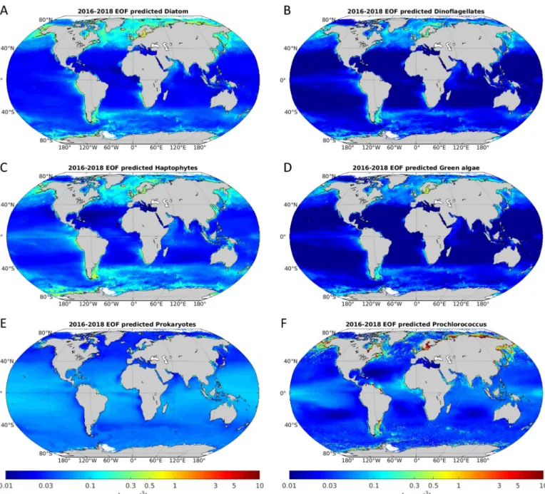
Fig. 6illustrates the global mean distribution Chl-aconcentration of each PFT, based on the monthly PFT products derived from the merged Rrsproducts with 25 km resolution from 2002 to 2012. Diatom Chl-a concentrations are generally higher in high latitudes, marginal seas and coastal upwelling regions but are much lower in the tropical regions and extremely low in the subtropical gyres. The typical diatom abundant regions are higher than 40°N (North Atlantic, Bering Sea and Labrador Sea up to the Arctic Ocean), the Patagonian upwelling and most part of the Southern Ocean. The average Chl-aconcentration of diatoms over the globe is ~0.08 mg m⁻³. Chl-aconcentration of dinoflagellates is low nearly over the whole globe (~0.02 mg m⁻³) but higher in the Arctic Ocean and Patagonian upwelling. Haptophytes with a global average Chl-aof 0.09 mg m⁻³follow in distributions of the diatoms but have more spread regions of high Chl-ain the high latitudes, waters near the coasts, and equatorial regions (such as the west coast of Africa). Chl-aconcentration of green algae (global average of 0.03 mg m⁻³) is found typically higher in the Arctic and the near coast oceans around the southern part of South America. Prokaryotes and Prochlorococcusshow distinctly different distribution features from the other four PFTs. Prokaryotes with a global average Chl-aconcentration of 0.07 mg m⁻³are much more abundant in the subtropical regions but also substantially contribute (~5–30% of TChl-a) in the Arctic Ocean.

Waters such as the Baltic Sea, the east coast of China, and the west coast of Africa (around 5°S and 10–20°N) show very prominent abundance of prokaryotes.Prochlorococcusare generally very low on a global scale (global average 0.03 mg m⁻³), especially in high latitude waters (not really detectable), slightly higher in subtropical regions and apparently abundant in some parts of the west coast of Africa similar to prokaryotes. Distribution ofProchlorococcusis supported by previous findings (Flombaum et al., 2013). Their quantitative model based on a large number of observations well defined the assessment of the Pro- chlorococcusabundance and the results match well our retrievals. In general the global average Chl-aconcentrations of the PFTs retrieved from our study are consistent with those from Hirata et al. (2011), except that prokaryotes Chl-a is higher (0.07 mg m⁻³ in our study versus 0.04 mg m⁻³fromHirata et al., 2011), mainly due to our ele- vated Chl-aprediction in the subtropics for prokaryotes. To illustrate the changes in the PFT Chl-a distribution with seasons, the monthly climatological products of each PFT are provided in Figs. S2-S7 in the supplementary document. For instance, diatom blooms are mainly detected during early summer in the Southern Ocean (December–Jan- uary) and in the subarctic and Arctic waters (May–June). Haptophytes show similar seasonal changes in high latitudes as diatoms, but highly increase during the summer season in the equatorial Atlantic. A strong prokaryotic enhancement is also found during July–August at the west coast of South Africa.

Distribution of TChl-a retrieved by the EOF-based algorithm is

(11)

presented in comparison to the GlobColour merged ocean chlorophyll products (mean over all years in Fig. 7, and climatological monthly mean in Figs. S8–S9). The ten-year mean of our EOF-based predicted TChl-a is generally in good agreement considering the distribution patterns with the standard products, though it is clearly seen that the EOF-based TChl-ashows higher/lower values in the subtropical gyres/

coastal waters than the standard products. This was however expected, as the EOF-based retrieval models based on matchups already showed an over-/under-estimation for lower/higher values for all the retrieved variables/PFTs, as illustrated in Fig. 5. This flattening effect of the prediction is most prominent in prokaryotes and Prochlorococcus, of which the EOF-based models present the weakest correlation. An accurate retrieval of prokaryotic phytoplankton or its corresponding marker pigments (zeaxanthin, divinyl Chl-a) has always been a chal- lenge so far (e.g.,Bracher et al., 2015;Losa et al., 2017), as the picophytoplankton Chl-aconcentrations are usually globally very low, even when dominating in oligotrophic oceans. This results in a narrow variation range and low variability in their concentrations compared to

other PFTs, and also in a weak imprint on the spectral shape which are limited for the detection via the spectral analysis. An exception is that in the Baltic Sea prokaryotes can have high Chl-a concentrations especially during blooms. This is also reflected in our retrievals, though there are no matchups available included in the EOF analysis.

3.3. Evaluation of the EOF-based PFT products 3.3.1. Inter-comparison with other PFT/PSC products

To evaluate our retrieval algorithm, the derived Chl-aconcentrations of diatoms, haptophytes and prokaryotes were compared with SynSenPFT Chl-aof diatoms, coccolithophores and cyanobacteria (Losa et al., 2017) and Chl-aof three PSCs (micro- >20 μm, nano- 2–20 μm, and picophytoplankton <2 μm,Sieburth et al., 1978) obtained with the PSC model ofBrewin et al. (2010, 2015). Both SynSenPFT and PSC products developed within the frame of the SynSenPFT project (Losa et al., 2017) were available globally at 4 km daily resolution over the period from 2002 to 2012. Prior to the inter-comparison, both products Fig. 6.Ten-year mean distribution (July 2002–April 2012) of the PFT Chl-aconcentration for (A) diatoms, (B) dinoflagellates, (C) haptophytes, (D) green algae, (E) prokaryotes, and (F)Prochlorococcusretrieved by EOF-based algorithm from merged monthly Rrsproducts at nine bands.

(12)

were binned to monthly averages and re-gridded to 25 km resolution, to be consistent with our EOF-based PFT products. For simplification, in the following text the SynSenPFT derived Chl-aconcentrations of diatoms, coccolithophores, and cyanobacteria are denoted as dia-Syn- SenPFT, coc-SynSenPFT, and cya-SynSenPFT, respectively; the Chl-a concentrations of micro-, nano- and picophytoplankton derived from PSC model are denoted as c-micro, c-nano, and c-pico, respectively. The EOF-based Chl-aproducts of the other two PFTs, green algae andPro- chlorococcuswere compared to those derived by OC-PFT method proposed byHirata et al. (2011)using GlobColour AVW merged TChl-a monthly 25-km products as input for the same period (2002–2012).

Dinoflagellates were not considered for comparison as the OC-PFT derived dinoflagellates showed very poor validation result (Hirata et al., 2011). It is noteworthy that OC-PFT also allows the retrieval of Chl-a concentrations of diatoms, haptophytes and prokaryotes, but as they are intrinsic in the SynSenPFT products (Losa et al., 2017) they were not included as separate products for the inter-comparison.

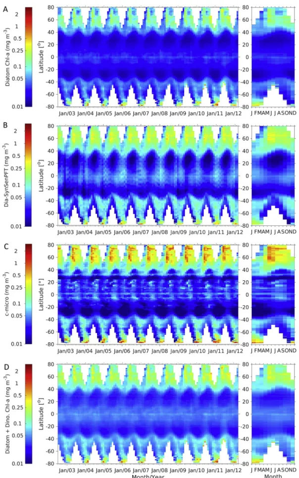
FollowingLosa et al. (2017), the time-latitude Hovmöller diagrams were generated covering the monthly means from 2002 to 2012 of the different PFT/PSC products. Since globally the Chl-aconcentration is typically log-normally distributed (Campbell, 1995), all averaging was done in logarithmic space and then back-transformed to the original scale. The Hovmöller diagrams are presented inFigs. 8–11, where the left side of each subplot shows the monthly variation during the ten- year period (2002–2012), and the right side shows the climatological annual cycle. Since different studies tend to provide different retrieval information in terms of phytoplankton composition, the optimal way for the inter-comparison is to select the variables carrying the most similar PFT information, but one has to keep in mind that the products compared here are not always representing exactly the same quantities.

Diatoms derived from our study (Fig. 8A) and dia-SynSenPFT (Fig. 8B) show similar distributions with both lowest diatom Chl-a concentration in the subtropical regions especially in the gyres and higher concentration in high latitudes. Compared to dia-SynSenPFT, the EOF-based diatoms show generally lower Chl-ain the polar and tropical regions, however they indicate the same blooming periods for diatoms in May–June in the Arctic and December–January in the Southern Ocean. Dia-SynSenPFT presented distinct higher Chl-a from 10°S to 10°N during December to February 2005–2006, 2007–2008 and 2010–2011 than other years, whereas the change between the years is not evident in either our results or the c-micro products (Fig. 8C). Since microphytoplankton contain not only diatoms but also other micro-size phytoplankton such as dinoflagellates, the sum of EOF-based diatoms and dinoflagellates was also shown (Fig. 8D), presenting similar seasonal variation to c-micro but higher/lower Chl-a in the gyres/high latitudes.

Before comparing the EOF-based haptophytes to other products, it should be noted that coccolithophores are a main contributing PFT to haptophytes, while haptophytes are a part of nanophytoplankton, with the latter containing alsoPhaeocystis, cryptophytes, and a few other groups. Haptophytes derived from our study (Fig. 9A) are well consistent with coc-SynSenPFT (Fig. 9B), although again our retrievals show a relatively mild pattern with lower Chl-ain high latitudes and the 10°S-10°N equator belt. Chl-aconcentration of coc-SynSenPFT from 10°N to 40°N during the summer time is significantly higher, but this pattern is not found in either our products or c-nano. Our haptophytes present similar distribution with c-nano (Fig. 9c) but lower Chl-ain the high latitudes and equatorial regions as expected. The climatological annual cycles of both are in very good agreement in the Southern Ocean, while in the Arctic c-nano shows much Chl-aenhancement in May–July. In addition, c-nano spreads more to the north until 25°N from the equator. However, caution should be taken since our DPA derived haptophytes contain only their nanophytoplankton fraction while their picophytoplankton fraction is neglected, whereasBrewin et al. (2015)consider part of the haptophytes in the picophytoplankton group when TChl-ais below 0.08 mg m⁻³.

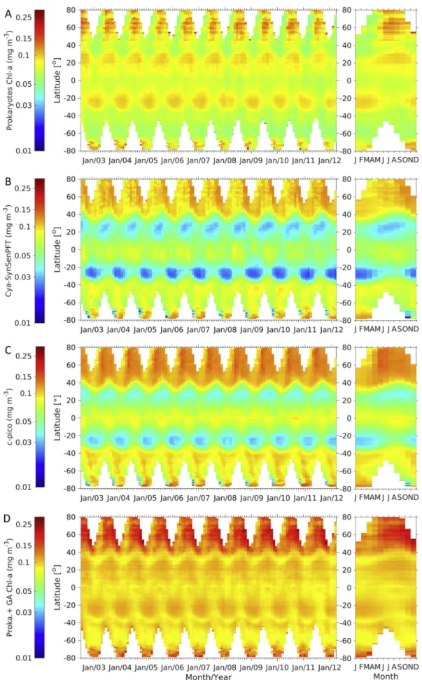
The overall Chl-a concentration of our EOF-based prokaryotes (Fig. 10A) is generally low (0.03–0.20 mg m⁻³), but higher concentrations are found in the subtropical regions, only slightly lower than the maxima in the Arctic and in the Southern Ocean from 70°S to 80°S during the summer. On the contrary, both distributions of cya- SynSenPFT (Fig. 10B) and c-pico (Fig. 10C) show the lowest Chl-ain the gyres. Similar seasonality (with little changes) between the cya-Syn- SenPFT and c-pico is observed at the mid- to high latitudes, while the EOF-based prokaryotes show slightly lower Chl-amaxima as well as a different seasonal change in the Arctic, which have a clear elevation in Chl-afrom spring to summer. It is noteworthy that the cyanobacteria derived from SynSenPFT include all the prokaryotic phytoplankton (Losa et al., 2017) which should thus be the same product as our EOF retrieved prokaryotes. The product of c-pico fromBrewin et al. (2015) contains not only prokaryotes but also other picoeukaryotic phytoplankton (green algae and pico-sized haptophytes), therefore we also presented inFig. 10D the sum of the prokaryotes and green algae Chl-a from our study, which shows much higher Chl-a concentration in general compared to c-pico, simply due to the predictions of high Chl-a of prokaryotes in the subtropical regions. Nevertheless, the high prokaryotes Chl-aconcentrations in the subtropical regions are not only shown in our study, but are also found in the cyanobacteria simulated by NASA Ocean Biogeochemical Model (NOBM), which is a global biogeochemical model with coupled circulation and radiative models (Gregg, 2002;Gregg and Casey, 2007, figure not shown here but can be found inLosa et al., 2017). However, our prokaryotic phytoplankton Fig. 7.Ten-year mean distribution (July 2002–April 2012) of (A) TChl-aconcentration retrieved by EOF-based algorithm from merged monthly Rrsproducts at nine bands and (B) GlobColour AVW merged TChl-aconcentration based on open ocean L2 chlorophyll products from SeaWIFS, MODIS and MERIS sensors.

(13)

Fig. 8.Hovmöller diagrams of Chl-aconcentrations of (A) diatoms derived from our study, (B) dia-SynSenPFT (Losa et al., 2017), (C) c-micro derived from PSC method (Brewin et al., 2015), and (D) sum of diatoms and dinoflagellates (Diatom + Dino.) from our study.

(14)

retrieval performance still needs to be further improved by potentially scaling the low concentration range or using non-linear prediction models.

Hovmöller diagrams of green algae andProchlorococcusChl-aconcentrations derived by our study (Fig. 11A–B) are presented in comparison with those from OC-PFT (Hirata et al., 2011,Fig. 11D–E). Green algae in both products show distinct seasonality but Chl-aconcentrations of green algae from our study are generally lower than those from OC-PFT (except for the subtropical regions), especially in the Arctic where OC-PFT shows enhanced green algae from late spring to early winter, whereas the EOF-based green algae show the lowest Chl-a during summer and increase in autumn to winter.ProchlorococcusChl-a is generally very low (< 0.1 mg m⁻³) for both products with quite different patterns presented. The EOF-based Prochlorococcus Chl-a concentrations are higher in mid- to low latitudes but lower in polar regions, corresponding to previous findings byFlombaum et al. (2013),

while the OC-PFTProchlorococcusshows higher Chl-ain the Southern Ocean which is outside the known distribution range and likely caused by undersampling of the in situ data (Hirata et al., 2011). Dino- flagellates show similar distribution with diatoms but with much lower Chl-aconcentration, which is almost neglectable in subtropical regions and only higher than 0.05 mg m⁻³in higher than 40°N with clear seasonality observed (Fig. 11C). However, an equivalent product is still necessary for dinoflagellates evaluation.

3.3.2. PFT Chl-a dominance comparison with PHYSAT products We compared the PFT Chl-adominance derived from our study for the period of 2002–2012 to the PHYSAT product from 1997 to 2006 (Alvain et al., 2008) which empirically relates the radiance anomaly to specific dominant phytoplankton groups. It is worth noting that the periods of the two compared products do not coincide, because we could only obtain the 12-month PHYSAT climatology data from 1997 to Fig. 9.Hovmöller diagrams of Chl-aconcentrations of (A) haptophytes derived from our study, (B) coc-SynSenPFT (Losa et al., 2017), and (C) c-nano derived from PSC method (Brewin et al., 2015).

(15)

Fig. 10.Hovmöller diagrams of Chl-aconcentrations of (A) prokaryotes derived from our study, (B) cya-SynSenPFT (Losa et al., 2017), (C) c-pico derived from PSC method (Brewin et al., 2015), and (D) sum of prokaryotes and green algae (Proka. + GA) from our study. Note that the color scale is different fromFigs. 8–9.