The interplay of thermodynamics and ocean dynamics during ENSO growth phase

https://doi.org/10.1007/s00382-020-05552-4

The interplay of thermodynamics and ocean dynamics during ENSO growth phase

Tobias Bayr¹  · Annika Drews^1,2 · Mojib Latif^1,3 · Joke Lübbecke^1,3

Received: 30 January 2020 / Accepted: 18 November 2020 / Published online: 2 December 2020

© The Author(s) 2020

Abstract

The growth of El Niño/Southern Oscillation (ENSO) events is determined by the balance between ocean dynamics and thermodynamics. Here we quantify the contribution of the thermodynamic feedbacks to the sea surface temperature (SST) change during ENSO growth phase by integrating the atmospheric heat fluxes over the temporarily and spatially varying mixed layer to derive an offline “slab ocean” SST. The SST change due to ocean dynamics is estimated as the residual with respect to the total SST change. In observations, 1 K SST change in the Niño3.4 region is composed of an ocean dynamical SST forcing of + 2.6 K and a thermodynamic damping of − 1.6 K, the latter mainly by the shortwave-SST (− 0.9 K) and latent heat flux-SST feedback (− 0.7 K). Most climate models from the Coupled Model Intercomparison Project phase 5 (CMIP5) underestimate the SST change due to both ocean dynamics and net surface heat fluxes, revealing an error compensation between a too weak forcing by ocean dynamics and a too weak damping by atmospheric heat fluxes. In half of the CMIP5 models investigated in this study, the shortwave-SST feedback erroneously acts as an amplifying feedback over the eastern equatorial Pacific, resulting in a hybrid of ocean-driven and shortwave-driven ENSO dynamics. Further, the phase locking and asymmetry of ENSO is investigated in the CMIP5 model ensemble. The climate models with stronger atmospheric feedbacks tend to simulate a more realistic seasonality and asymmetry of the heat flux feedbacks, and they exhibit more realistic phase locking and asymmetry of ENSO. Moreover, the almost linear latent heat flux feedback contributes to ENSO asymmetry in the far eastern equatorial Pacific through an asymmetry in the mixed layer depth. This study suggests that the dynamic and thermodynamic ENSO feedbacks and their seasonality and asymmetries are important metrics to consider for improving ENSO representation in climate models.

1 Introduction

The El Niño/Southern Oscillation (ENSO) is the dominant mode of tropical climate variability on interannual time- scales and driven by a complex interplay between amplify- ing (positive) and damping (negative) coupled ocean-atmos- phere feedbacks (e.g. Jin et al. 2006). ENSO is associated with extreme weather such as heavy precipitation events and droughts in the tropical Pacific region and beyond (e.g.

Philander 1990; Yeh et al. 2018). During its warm (cold)

phase, El Niño (La Niña), the sea surface temperature (SST) is warmer (colder) than normal in the eastern and central equatorial Pacific. These warm (cold) SST anomalies are related to anomalously high (low) upper-ocean heat content and eastward (westward) advection of warm (cold) water.

The onset of El Niño events are often triggered by westerly wind bursts over the western equatorial Pacific that force eastward propagating downwelling oceanic Kelvin waves that warm the SST in the central and eastern equatorial Pacific, where the thermocline is shallow (e.g. Lengaigne et al. 2004; Fedorov et al. 2015; Neske and McGregor 2018;

Timmermann et al. 2018). This initial warming is ampli- fied by the Bjerknes feedback loop, i.e., the equatorial SST warming in the east weakens the zonal wind over the west- ern Pacific, which then results in a deeper thermocline that reinforces the initial positive SST anomaly in the central and especially eastern equatorial Pacific.

The growth of SST anomalies is damped by the heat flux feedback consisting mainly of the negative shortwave-SST

* Tobias Bayr tbayr@geomar.de

1 GEOMAR Helmholtz Centre for Ocean Research Kiel, Düsternbrooker Weg 20, 24105 Kiel, Germany

2 Department of Environment and New Resources, SINTEF Ocean AS, Trondheim, Norway

3 Faculty of Mathematics and Natural Sciences,

Christian-Albrechts-University of Kiel, 24105 Kiel, Germany

feedback and the negative latent heat flux-SST feedback (Lloyd et al. 2009). The negative shortwave-SST feedback is caused by the eastward shift of atmospheric deep convec- tion during an El Niño event and dominates the heat flux feedback over the western and central equatorial Pacific, where the largest shift in convection is observed (Lloyd et al.

2011). The negative latent heat flux-SST feedback relates to an increased evaporation due to warmer SSTs during El Niño events and is strongest over the eastern equatorial Pacific, where the SST change is largest (Lloyd et al. 2011).

The same amplifying and damping feedbacks operate during La Niña events, but the anomalies have opposite signs. In association with the longitudinal shift of the rising branch of the Walker Circulation over the western and central Pacific, there is a pronounced asymmetry in the shortwave feedback between El Niño and La Niña (Lloyd et al. 2012; Bellenger et al. 2014; Bayr et al. 2018). The shortwave feedback varies both in amplitude and location, thus is stronger and operates more eastward during El Niño than during La Niña (Bayr et al. 2018). The latent heat flux feedback over the eastern Pacific is mostly linear (Lloyd et al. 2011).

ENSO events typically grow during boreal summer and autumn, reach their maximum around the end of the year and decay in the following boreal spring (Timmermann et al. 2018). This seasonal phase locking of ENSO can be explained by the seasonality of the amplifying and damp- ing feedbacks. During ENSO growth in boreal summer and autumn, the positive coupled feedbacks reach their maxi- mum while the thermodynamic damping is at its minimum.

This can be explained by the seasonal outcropping of the thermocline in the east (Galanti et al. 2002), the more equa- torward position of the Intertropical Convergence Zone (Tziperman et al. 1998) and the reduction in the negative cloud feedbacks (Dommenget and Yu 2016). During the ENSO decay phase in the following spring, the thermo- dynamic damping reaches its maximum while the positive coupled feedbacks are at their minimum (e.g. Tziperman et al. 1998; Galanti et al. 2002; Dommenget and Yu 2016;

Wengel et al. 2018).

One important aspect of ENSO is the asymmetry between El Niño and La Niña, i.e., that SST anomalies during El Niño events are usually stronger and located further to the east than during La Niña events (Takahashi et al. 2011;

Dommenget et al. 2013; Capotondi et al. 2014; Timmer- mann et al. 2018). The causes of this asymmetry are still under debate. Important contributors are: nonlinearities in the wind-SST feedback (Frauen and Dommenget 2010;

Karamperidou et  al. 2017) and in the shortwave-SST feedback (Lloyd et al. 2009, 2011, 2012; Bellenger et al.

2014), stronger subsurface-surface coupling during El Niño (Meinen et al. 2000; Lübbecke and McPhaden 2017), larger dynamical ocean response per unit zonal wind stress change during El Niño (Im et al. 2015), nonlinear time-averaged

ocean response to tropical instability waves (Imada and Kimoto 2012), and state-dependent stochastic noise (Levine et al. 2016; Hayashi and Watanabe 2017). Teleconnections from the tropical Atlantic and Indian Oceans (Okumura and Deser 2010; An and Kim 2018) and the extratropics also may contribute to ENSO asymmetry (Li et al. 2007; Wu et al. 2010).

State-of-the-art climate models still exhibit severe defi- cits in simulating important ENSO properties such as the seasonal phase locking (Bellenger et al. 2014; Wengel et al.

2018) or the asymmetry between El Niño and La Niña (Dommenget et al. 2013; Zhang and Sun 2014; Timmer- mann et al. 2018). These deficiencies can be partly explained by a cold equatorial SST bias present in many climate models, which shifts the models into a La Niña-like mean state with a too western position of the rising branch of the Walker Circulation. The wind-SST feedback and heat flux- SST feedback are strongly underestimated in these models (Kim et al. 2014; Wengel et al. 2018; Bayr et al. 2018). As the position of the rising branch of the Walker Circulation determines the strength of both atmospheric feedbacks (Bayr et al. 2020), models that underestimate the wind-SST feed- back also tend to underestimate the heat flux-SST feedback, with error compensation between these two feedbacks (Guil- yardi et al. 2009; Bellenger et al. 2014; Kim et al. 2014; Bayr et al. 2018, 2019). Bayr et al. (2019) investigated in detail how this error compensation hampers the simulated ENSO dynamics in climate models: they analyzed within the Bjerk- nes Stability (BJ) index framework (Jin et al. 2006) the posi- tive thermocline, zonal advection and Ekman feedbacks and the negative thermodynamic damping. All four feedbacks are weaker if the atmospheric feedbacks are underestimated, but the resulting total BJ index is not too different from that in models with strong atmospheric feedbacks. To quantify the error compensation, they also calculated the contribution of the atmospheric heat fluxes to the SST tendency during the ENSO growth phase. They report that in many climate models ENSO is a hybrid of ocean-driven and shortwave- driven ENSO dynamics, in equal proportions in the most biased models. This already was suggested by previous stud- ies (Dommenget 2010; Dommenget et al. 2014; Bayr et al.

2018). Bayr et al. (2019) quantified for the first time the contribution of the shortwave feedback to the SST tendency.

This study is part of a series of studies that focus on the ENSO atmospheric feedbacks: Bayr et al. (2018) described the relation between the equatorial SST bias, the mean-state Walker Circulation, and the ENSO atmospheric feedback strength. Bayr et al. (2019) revealed the effect of the error compensation of the atmospheric feedbacks on simulated ENSO dynamics and the hybrid nature of ENSO dynamics in biased models. Finally, Bayr et al. (2020) showed that also in uncoupled models the atmospheric mean state is impor- tant for atmospheric feedback strength and explained the

difference in atmospheric feedback strength between uncou- pled and coupled simulations.

The aim of this study is to better understand the interplay of thermodynamics and ocean dynamics during the ENSO growth phase in observations, reanalysis products and in cli- mate models participating in the Coupled Model Intercom- parison Project phase 5 (CMIP5). We employ the offline slab ocean SST method introduced in Bayr et al. (2019) and apply it more accurately by using a temporally and spatially vary- ing mixed layer depth (MLD) instead of a constant MLD.

This enables a better understanding of the role of the heat fluxes in ENSO dynamics, as the MLD considerably varies with the seasons and during ENSO events, especially in the eastern equatorial Pacific where the MLD is shallow and therefore has a stronger influence on the SST. Further, the importance of the atmospheric feedbacks for the seasonal phase locking and the asymmetry of ENSO is investigated.

This study is organized as follows: in Sect. 2, we describe the data and methods. Section 3 provides the results pertain- ing to the interplay of thermodynamics and ocean dynamics during the ENSO growth phase in the different datasets. In Sect. 4, we investigate the seasonal ENSO phase locking and in Sect. 5, the ENSO asymmetry. The results are sum- marized and discussed in Sect. 6.

2 Data and methods

We use observed SSTs for the period 1958–2018 from Had- ISST (Rayner et al. 2003), zonal wind stress and heat fluxes for the period 1958–2001 from ERA40 (Uppala et al. 2005) and for the period 1979–2018 from ERA-Interim reanal- ysis (Simmons et al. 2007). Observed heat fluxes for the period 1979–2018 are from the Wood Hole Oceanographic Institute data set, also referred to as OA Flux data set (Yu et al. 2008). OA Flux uses shortwave and longwave fluxes from ISCCP (Rossow and Schiffer 1999) for the period 1979–2001 and from CERRES (Wielicki et al. 1996) for the period 2002–2018. The mixed layer depth (MLD) is calculated from ocean temperature from SODA reanaly- sis (Carton and Giese 2008) for the period 1958–2001 and from observations using HadEN4.2 (Good et al. 2013) for the period 1979–2018. The MLD is defined as the depth at which the ocean temperature has decreased by 0.2 K com- pared to the surface. Further, we set the minimum MLD to 10 m, as with the 0.2 K criterion some models have MLDs of even less than 1 m. As we divide by the MLD to com- pute the offline slab ocean temperature, such small MLDs would give unrealistically large temperature changes. The 10 m limit can be justified by the fact that observed MLDs in the tropical Pacific less than 10 m are very rare. Further, most ocean components of the CMIP5 models only have one vertical level in the upper 10 m and the depth of the first

layer determines the possible minimum MLD. Finally, the shortwave radiation warms the upper 50 m of the ocean inde- pendent of the MLD, as e.g. two thirds of the surface solar irradiance penetrates below 10 m (Hieronymi et al. 2012).

From CMIP5, we analyze the twentieth century historical simulation (1900–1999) for a set of 38 models. Only those models are considered for which the heat fluxes, zonal wind stress and ocean temperatures are available (see Fig. 3 for a list of models). The MLD was calculated in the same way as for observations using the 0.2 K difference criterion. All model data is interpolated on a regular 2.5° × 2.5° grid. We use monthly-mean anomalies relative to seasonally vary- ing climatology and the data from each calendar month is detrended separately.

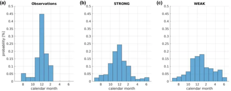
ENSO events are defined according to Trenberth (1997) as time periods in which the five-month running mean of Niño3.4 SST is above the ± 0.5 standard deviation thresh- old for at least 6 consecutive months. We determine the time of the maximum for each event separately (Fig. 1a), and long ENSO events like the 1998/1999 La Niña with two maxima are considered as two events if there are more than 11 months between the two peaks. The Niño3 region is defined as 90°W–150°W and 5°S–5°N, the Niño3.4 region as 120°W–170°W and 5°S–5°N, and the Niño4 region as 160°E–150°W and 5°S–5°N.

The seasonal phase locking of ENSO is measured by the phase locking index proposed by Bellenger et al. (2014). It is the ratio between the Niño3.4-averaged standard devia- tion of the SST in the months November, December, Janu- ary (NDJ, high variability months) divided by the average standard deviation in the months April, May, June (AMJ, low variability months). Phase locking of the net heat flux, shortwave and latent heat flux feedback is defined as the dif- ference between the average feedback in February, March, April (FMA, strongest damping) minus the average feedback in September, October, November (SON, weakest damping) as shown in Sect. 4.

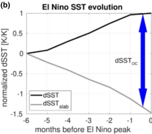
The thermodynamic contribution to the SST change dur- ing ENSO growth is calculated by integrating the net heat flux Q_net, similar to Drews and Greatbatch (2016). Here, the integration is performed over the 6 months preceding the maximum of each ENSO event, as 6 months is the average growth length in observations (Fig. 1a, b):

where cp= 4000 J kg⁻¹ K⁻¹ is the specific heat capacity at constant pressure of sea water, ρ = 1024 kg m⁻³ the average density of sea water, H the temporally and spatially varying MLD in meters, and t time in months. We normalize the SST change (dSST) and the SST change caused by the heat fluxes (dSST_slab) by dSST at the maximum (t = 0), yielding an SST (1) dSST_slab=

1 c_p⋅𝜌∫

t=0 t=−6

Q_net H dt

change per Kelvin warming (Fig. 1b) and enabling com- parison of the contributions in the individual climate models irrespective of their ENSO amplitude. We also perform the integration with the shortwave (SW), longwave (LW), sensi- ble (SH) and latent heat (LH) flux in order to estimate their contribution to the SST tendency. As a simplification, we integrate the full SW anomalies to the dSST_slab even if the MLD is shallower than the SW penetration depth. The effect of this simplification is negligible, as such shallow MLDs are quite rare and the heat flux feedback in these regions (mainly the eastern equatorial Pacific) is dominated by the LH feedback. Finally, as the observed SST change is the balance of the SST changes due to ocean dynamics (dSST_oc) and net heat flux (dSST_slab), we can estimate the contribu- tion of the ocean dynamics from the results above (Fig. 1b):

In this way, it is possible to quantify the contributions of thermodynamics and ocean dynamics during ENSO growth and to describe their interplay.

To estimate the uncertainty in the SST change by the heat fluxes, we apply a bootstrapping approach. We ran- domly choose 1000 times only two thirds of the ENSO events and calculate the SST change. We show the uncer- tainty as error bars, indicating the 90% quantile of the estimated values. In a similar manner, we estimate the uncertainty of the seasonal variation of the SST variability (2) dSST≈dSST_oc+dSST_slab

(3) dSST_oc≈dSST−dSST_slab

and the mean MLD, but here by randomly choosing 1000 times two thirds of the years.

3 ENSO growth in observations and CMIP5 models

We apply Eq. (1) to the observations and reanalysis prod- ucts over the Niño3.4 region. This yields a damping of

− 1.6 ± 0.2 K by the net heat flux per Kelvin change in SST (dSST_slab(Q_net), Fig. 2). The damping is primarily caused by a negative shortwave (dSST_slab(SW), − 0.9 ± 0.1 K/K) and latent heat flux-SST feedback (dSST_slab(LH),

− 0.7 ± 0.1 K/K), while the contributions of the longwave radiation and sensible heat flux are small (Fig. 2). Accord- ing to Eq. (3), the ocean dynamics (dSST_oc) would yield an amplifying contribution of about + 2.6 K ± 0.2 K per 1 K SST change, as the rest is damped away by heat fluxes (Fig. 2). The error bars in Fig. 2 indicate the uncertainty of each feedback calculated by the bootstrapping approach described above.

An analysis similar to that shown in Fig. 2 for obser- vations is performed for the CMIP5 models. In agreement with previous studies by Lloyd et al. (2009, 2011, 2012) and Bayr et al. (2018, 2019), we find that in the Niño3.4 region differences in the net heat flux (Q_net) feedback among the CMIP models is mostly due to differences in the shortwave (SW) feedback (Fig. 3a). Despite a marked spread in MLD in the Niño3.4 region (Fig. 3c), we find a strong correlation between dSST_oc and dSST_slab(SW) in the models, amounting

1980 1985 1990 1995 2000 2005 2010 2015 year

-3 -2 -1 0 1 2 3

SSTa [K]

5 month running mean of Nino3.4 SST

(a) (b)

Nino3.4 start growth peak decay end threshold

Fig. 1 a Five month running mean of SST anomalies in the Niño3.4 region from 1979 to 2018 in HadISST; the black horizontal lines mark the threshold for ENSO events, which has to be passed for at least 6 consecutive months; green circles mark the beginning of an ENSO event, yellow the growth period, red the maximum, cyan the decay phase and blue the end; b in black the SST evolution (dSST) in Niño3.4 region averaged over all El Niño events from 6  months

before the maximum till the maximum, normalized by the dSST at the maximum; in gray the evolution of the Offline Slab Ocean SST (dSST_slab), calculated by the integration of the net heat flux anomalies to the local mixed layer depth, as described in Eq. (1); the blue arrow indicates the SST change by ocean dynamics (dSST_oc), estimated from the difference between dSST and dSST_slab in Eq. (3)

to − 0.73 (Fig. 3b). This strong correlation highlights the error compensation between the underestimated wind-SST forcing and the underestimated heat flux-SST damping in many CMIP5 models (Fig. 3d). Bayr et al. (2019) showed that models with strongly underestimated wind-SST feed- back can have ENSO statistics that at first glance are not too different from observations but due to very different ENSO dynamics. These models exhibit hybrid wind-driven and shortwave-driven ENSO dynamics, as the weaker ocean dynamical forcing is compensated by an erroneously positive SW feedback that acts as an additional forcing (Fig. 3b). In the most strongly biased models, the SW feedback contrib- utes to the SST change with a similar magnitude as the ocean dynamics (Fig. 3b). The strength of dSST_slab(SW) is domi- nated by the strength of the SW feedback, with a correla- tion of 0.93 (not shown), which explains why dSST_slab(SW) and MLD are uncorrelated (Fig. 3c). The three outliers in Fig. 3b (model number 14, 15 and 33) have a stronger than average latent heat flux (LH) feedback and shallower than average MLD. Therefore, the dSST_oc is stronger in these models than in models with a similar dSST_slab(SW), due to a stronger dSST_slab(LH). We find that the model spread in the LH feedback over the Niño3.4 region is generally much smaller than the spread in SW feedback (10 W/m² in the former in comparison to 30 W/m² in the latter) and that there is no significant correlation between the LH feedback and the Q_net feedback (not shown). Thus, the error compensation between the SW feedback and the wind feedback is very

clear in the Niño3.4 region during the ENSO growth phase, even though the models differ substantially in MLD.

To elucidate the effect of the error compensation on the simulated SST change in the Niño3.4 region during the ENSO growth phase, we define two sub-ensembles:

STRONG (indicated in red in Fig. 3) and WEAK (indicated in blue). The sub-ensembles are defined according to their combined atmospheric feedback strength, with STRONG

> 0.55 and WEAK < 0.55 of the observed atmospheric feedback strength. The combined atmospheric feedback strength is defined as the average of the wind and heat flux feedback, both normalized by the observed value. We use the combined atmospheric feedback strength for defining the sub-ensembles, as it is a measure of the error compensation between the two feedbacks and enables separating the mod- els into sub-ensembles in which dSST_slab(SW) acts either as damping (STRONG sub-ensemble) or erroneously as forcing (WEAK sub-ensemble) (Fig. 3b). The atmospheric feedback strength depends on the relative SST bias in the Niño4 region (Fig. 3e), as described in more detail in Bayr et al. (2018). The relative SST is defined with respect to the tropical Pacific (120° E–80°W, 30°S–30°N) area-mean SST and used to account for the different mean temperatures in the climate models, as tropical convection is more strongly related to relative SST than to absolute SST (Johnson and Xie 2010; Bayr and Dommenget 2013; Izumo et al. 2019).

Compared to observations, the STRONG sub-ensemble has quite realistic ENSO dynamics, with only 0.5 K/K weaker dSST_oc and dSST_slab(Q_net) (Fig. 4). From STRONG to WEAK, dSST_slab(Q_net) decreases from − 1.1 K/K to

− 0.2 K/K, with dSST_slab(SW) contributing most to the difference between the two sub-ensembles. The dSST_oc decreases similarly from + 2.1 K/K to + 1.2 K/K, while dSST_slab(SW) changes from a − 0.8 K/K damping to a + 0.6 K/K forcing, causing the hybrid nature of ENSO dynamics in models belonging to the WEAK sub-ensemble, with a large shortwave-driven component. The dSST_slab(LH) has a quite similar strength in both CMIP5 sub-ensembles (− 0.5 K/K and − 0.6 K/K in STRONG and WEAK, respec- tively) than in observations (− 0.7 K/K).

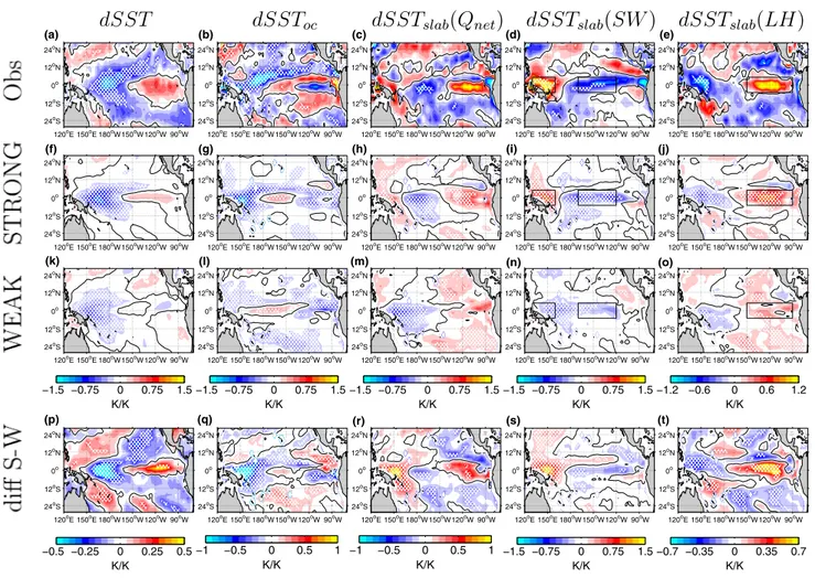
Performing the analysis at each grid point provides the patterns (Fig. 5) that are shown at the peak of the ENSO event (t = 0). As we will first focus on the strength of the dynamics in observations and CMIP5 sub-ensembles and later on the asymmetry between El Niño and La Niña, we show here the results for both El Niño and La Niña events together. Further, as the dSST_slab (in K) depends on both the heat flux strength (in W/m²) and the MLD, we show addi- tionally the equatorial heat flux strength for Q_net, SW and LH (in W/m²) and the equatorial MLD in Fig. 6. Thus, for clari- fication, when we refer, for example, to the Q_net feedback, the feedback in W/m² is meant, while dSST_slab(Q_net) is the

Oc Qnet SW LW SH LH

-2 -1.5 -1 -0.5 0 0.5 1 1.5 2 2.5 3

Normalized dSST [K/K]

SST change in Nino3.4

Fig. 2 Average SST change in the Niño3.4 region at the maximum of all ENSO events in an observation and reanalysis ensemble, due to ocean dynamics (blue bar), net heat flux (gray bar), shortwave radia- tion (yellow bar), longwave radiation (red bar), sensible heat flux (cyan bar) and latent heat flux (green bar); All values are normal- ized per 1 K total SST change in the Niño3.4 region; The errorbars indicate the 90% confidence interval estimated by a bootstrapping approach, as described in the methods section

effect of the heat flux feedback on SST in K, with temporar- ily and spatially varying MLD considered.

In observations, the SST change in the 6 months before the maximum of the ENSO event (dSST, Fig. 5a) exhibits its maximum to the west of the largest SST anomaly (not shown). The dSST_slab(Q_net) has its maximum over the eastern Pacific (Fig. 5c) and its pattern is similar to dSST_oc (Fig. 5b).

Largest dSST is in Niño3.4, because there the ocean dynami- cal forcing is strong while heat flux damping is weak. The strongest heat flux damping is observed over the eastern part of the basin. The dSST_slab(LH) dominates the damping in the eastern part of the Niño3 region (90°W–120°W, 5°S–5°N, Fig. 5e), while dSST_slab(SW) dominates the damping in the Niño3.4 and Niño4 regions (Fig. 5d). The dSST_slab(Q_net) (Fig. 5c) is much smaller in the western than in the eastern Pacific even though the SW feedback in the western Pacific (≈ − 20 W/m²/K, Fig. 6d) is stronger than the LH feedback over the eastern Pacific (≈ − 13 W/m²/K, Fig. 6g). This can

be explained by the shallower mixed layer in the eastern (20–30 m, Fig. 6j) relative to that in the central and west- ern Pacific (40–60 m, Fig. 6j). Therefore, the minimum of dSST_slab(SW) in the western Pacific, amounting to − 2 K/K, is half as strong as the minimum in dSST_slab(LH) in the eastern Pacific (Fig. 5d, e). The LW radiation is mostly of opposite sign with regard to the SW radiation but much weaker, and the SH contributes very little to dSST_slab(Q_net) (not shown).

We conclude from the above analyses: first, the Q_net feed- back is largest over the Niño3.4 region (− 20 W/m²) due to strong SW and LH damping (Fig. 6a, d, g), but dSST_slab(Q_net) is relatively weak there due to the deep MLD (Figs. 5c, 6j).

Second, while dSST is largest in the Niño3.4 region, dSST_oc is not (Fig. 5a, b). The situation is quite different in the east- ern part of the Niño3 region: the Q_net damping is weaker (between − 20 and − 10 W/m²/K, Fig. 6a), but due to a much shallower MLD (Fig. 6j), the dSST_slab(Q_net) has its maximum

-20 -10 0 10

Short wave feedback in Nino3.4 [W/m*m/K]

-20 -15 -10 -5 0

Heat flux feedback in Nino3.4 [W/m*m/K]

SW vs. Heat flux feedback

1

2

34

5 67

8 9

10 11

12

13

1415 16

17

18

19

2120

23 22

2425

262728 29 30

31

3233 34

35 36

3738 r = 0.93***

(a)

-1 0 1 2

dSST by SW feeback in Nino3.4 [K/K]

0 0.5 1 1.5 2 2.5 3

dSST by ocean dynamics in Nino3.4 [K/K]

dSST(SW) vs. dSST(oc)

1

2 34 5

67 89

10 11

12

13 14

15

1617

18 19

20 21 22 23 2425

26 27 28

29 30 31 32

33

34

35 36 37

38

r = -0.73***

(b)

DAMPING FORCING

-1 0 1 2

dSST by SW feedback in Nino3.4 [K/K]

-80 -70 -60 -50 -40 -30

MLD in Nino3.4 [m]

dSST(SW) vs. MLD

1 2 3

4 5

67 98111210

13

14 15 1617

18 19

20 21

22 23

2524 26

2728 29 31 30

32 33

34 3635

3738

r = 0.08

(c)

0.5 1 1.5

Wind stress feedback in Nino4 [10e-2 Pa/K]

-18 -16 -14 -12 -10 -8 -6 -4 -2 0 2

Heat flux feedback in Nino3 and Nino4 [W/m*m/K]

Wind vs. heat flux feedback

1 2

4 3 5

67

98 10

11 12 13

14 15

16 17 18

19 20

21

22 23

24 25 26 27

28 29

30

31

32 33

34 3536

37 38

r = -0.60***

(d)

0 0.2 0.4 0.6 0.8 1

Atmospheric feedbacks (normalized) -2

-1.5 -1 -0.5 0 0.5

rel. SST bias in Nino4 [K]

Atm. Feedbacks vs. SST bias

1 2

3 4 5

67 98 10

11 12

13

14

15 1716

18 20 19

21 22

23 2524

26 2827 29 30

31

32 33 34 3536

3837 r = 0.70***

(e)

Fig. 3 For observations/reanalysis and CMIP5 models in a net heat flux feedback in the Niño3.4 region on the y axis vs. the shortwave feedback in Niño3.4 region on the x axis; b SST change during ENSO events by ocean dynamics on the y axis vs. SST change by shortwave radiation on the x axis, both for the Niño3.4 region; c same as b, but here the mean mixed layer depth during ENSO growth phase on the y axis; d same as a, but here for the zonal wind stress-SST feedback in the Niño4 region on the x axis; e average strength of wind and heat

flux feedback, both normalized by the observed strength, on the x axis vs. relative SST bias in the Niño4 region on the y axis; The black line is the regression line between the CMIP5 models with the correlation given in the upper right/left corner, where 1, 2, 3 stars are indicat- ing a significant correlation on a 90%, 95% and 99% confidence level, respectively; the color of the numbers indicate the sub-ensembles with STRONG (red) and WEAK (blue) ENSO atmospheric feedbacks

in the east (Fig. 5c). The dSST_oc also has its maximum in the eastern part of the Niño3 region (Fig. 5b). However, dSST is much smaller there than in the Niño3.4 region due to stronger dSST_slab(Q_net) damping in the Niño3 region (Fig. 5a, c). In summary, the interplay between thermody- namics and ocean dynamics differs substantially between the Niño3.4 region and eastern part of the Niño3 region, and the difference in the MLD between these two regions is an important factor for this difference.

The two CMIP5 sub-ensembles on average simulate the ensemble-mean MLD quite realistically but exhibit a large spread between the models (grey shading in Fig. 6k, l) as already indicated in Fig. 3c). The spread in MLD is larg- est over the central Pacific and slightly larger in STRONG than in WEAK. The dSST is extending further to the west in WEAK than in STRONG (Fig. 5f, k), which becomes obvious in the difference between STRONG and WEAK (Fig. 5p). This more westward extension in the dSST pat- tern in WEAK in comparison to STRONG can be related to a decrease of dSST_slab(Q_net) over the central Pacific, which almost vanishes in WEAK (Fig. 5h, m, r). The pattern of the estimated dSST_oc (Fig. 5g, l, q) is quite realistic in STRONG but much weaker in WEAK. In WEAK, there is a secondary maximum in the west (Fig. 5l).

The differences in dSST_slab(Q_net) mainly result from dSST_slab(SW) (Fig. 5i, n, s), as its minimum is much fur- ther west in WEAK than in STRONG. Further, an area with a positive SST change emerges in the eastern Pacific in WEAK. The dSST_slab(LH) is a bit stronger in WEAK than in STRONG along the equator (Fig. 5j, o, t), but the

difference in dSST_slab(Q_net) is clearly dominated by the dif- ference in dSST_slab(SW) (Fig. 5r, s, t). When we compare the heat flux feedbacks and MLDs in the two sub-ensembles (second and third column in Fig. 6), we find that the differ- ence in dSST_slab(SW) is mainly caused by the SW feedback (Fig. 6e, f), as the mean MLD is quite similar in both sub- ensembles (Fig. 6k, l). Further, the LH feedback is quite similar in the two sub-ensembles (Fig. 6h, i), so that the difference in the Q_net feedback is dominated by the differ- ence in SW feedback (Fig. 6b, c). Finally, the changes in the SW feedback can be linked to a westward shift of the Pacific Walker Circulation from STRONG to WEAK due to a larger equatorial cold SST bias (Fig. 3e), which leads to the posi- tive SW feedback over the eastern Pacific in WEAK (Bayr et al. 2018, 2020). The influence of the error compensation between the underestimated wind and heat flux feedbacks on ENSO dynamics is largest in the Niño3.4 region, where the SST (in observations) is less damped in comparison to the eastern part of the Niño3 region and the largest differences in dSST_slab(SW) and dSST_oc occur. Therefore, only a weak dSST_oc forcing is required in models of the WEAK category to produce a sizeable SST anomaly.

In summary, ENSO dynamics in the Niño3.4 region differ substantially among the CMIP5 models, with only half of the models simulating a realistic interplay between thermodynamic and ocean dynamical feedbacks during the ENSO growth phase, while the other half exhibits a hybrid of ocean-driven and shortwave-driven ENSO dynamics due to an equatorial cold SST bias (Fig. 3). Further, the too west- ward extension of the ENSO-related SST anomaly pattern observed in many models can be explained by the too weak heat flux damping and too strong ocean dynamical forcing over the central and western equatorial Pacific.

4 Seasonal ENSO phase locking

The realistic simulation of the seasonal ENSO phase lock- ing is still a challenge (Bellenger et al. 2014; Wengel et al.

2018). In observations, there is a distinct peak in the occur- rence of maximum SST anomalies during ENSO events in December (Fig. 7a). In the CMIP5 models the distribution is much more spread over the calendar year (Fig. 7b, c).

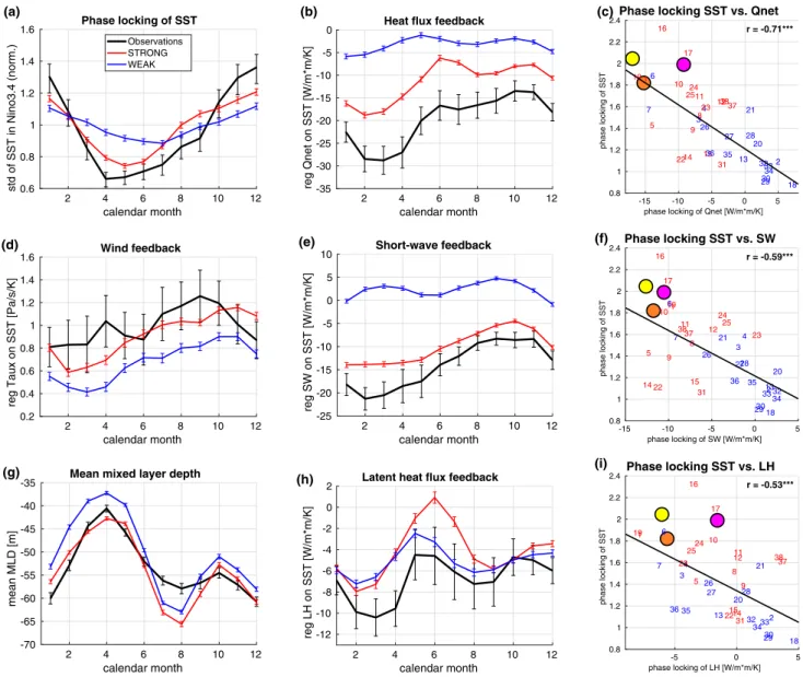
In STRONG, the probability of ENSO peaking in boreal spring is quite low but it is considerably higher in WEAK (Fig. 7b, c). The seasonal ENSO phase locking over the Niño3.4 region is simulated more realistically in STRONG than in WEAK (Fig. 8a). In agreement with Wengel et al.

(2018), the seasonal phase locking can be explained in observations by the maxima of the wind feedback in boreal autumn (Fig. 8d) and of the heat flux damping in boreal spring (Fig. 8b). The latter is mainly caused by the SW feed- back (Fig. 8e), but also to a minor part by the LH feedback

Obs STRONG WEAK

-2 -1 0 1 2 3 4

Normalized dSST [K/K]

SST change in Nino3.4

dSST_oc dSST_slab (Qnet) dSST_slab (SW) dSST_slab (LW) dSST_slab (SH) dSST_slab (LH)

Fig. 4 Same as Fig. 2, but here additionally for sub-ensembles of CMIP5 models with STRONG and WEAK atmospheric feedbacks, as indicated by the colors in Fig. 3); The values shown here are the averages over the boxes shown in Fig. 5; The errorbars indicate the 90% confidence interval estimated by a bootstrapping approach, as described in the methods section

(Fig. 8h). Observations (purple dot) and reanalysis data (yel- low and orange dot), however, do not agree on the seasonal variation of the LH feedback (Fig. 8i). The seasonal cycle of the MLD enhances the effect of the seasonal cycle of the SW and LH feedbacks, as the mixed layer is shallowest in boreal spring when these heat flux feedbacks are strongest (Fig. 8g).

The seasonality of the wind feedback is quite similar in the two sub-ensembles, but the averaged strength is larger for models in STRONG relative to those in WEAK (Fig. 8d).

With respect to the Q_net and SW feedbacks, the seasonality is pronounced in STRONG while there is less seasonality in WEAK (Fig. 8b, e). The seasonality of the LH feedback and MLD is similar in both sub-ensembles (Fig. 8g, h). Signifi- cant correlations exist in the model ensemble between the seasonal phase locking of SST and that of the Q_net feedback (− 0.71, Fig. 8c), the SW feedback (− 0.59, Fig. 8f), and the LH feedback (− 0.53, Fig. 8i). This suggests that the heat

flux damping plays an important role in the ENSO phase locking, as models with a stronger seasonality in the heat flux feedbacks tend to exhibit a stronger SST phase locking.

Those are not the only factors that influence the SST phase locking, as some models exhibit weak SST phase locking in the presence of a strong phase locking of the Q_net and SW feedbacks (e.g. models 14 and 22). Further, other models have a reasonable SST phase locking despite weak season- ality in the Q_net, SW and LH feedbacks (e.g. model 21), arguing for an importance of, for example, the wind-SST feedback.

5 ENSO asymmetry

ENSO asymmetry, i.e., the differences between the pat- tern of El Niño and La Niña events, is investigated next. In observations, the maximum of dSST is more in the east and

dSST dSST

dSST

(Q

) dSST

(SW ) dSST

(LH )

120^oE 150^oE180^oW150^oW120^oW90^oW 24^oS

12^oS 0^o 12^oN 24^oN

(a)

120^oE 150^oE180^oW150^oW120^oW90^oW 24^oS

12^oS 0^o 12^oN 24^oN

(b)

120^oE 150^oE180^oW150^oW120^oW90^oW 24^oS

12^oS 0^o 12^oN 24^oN

(c)

120^oE 150^oE180^oW150^oW120^oW90^oW 24^oS

12^oS 0^o 12^oN 24^oN

(d)

120^oE 150^oE180^oW150^oW120^oW90^oW 24^oS

12^oS 0^o 12^oN 24^oN

(e)

120^oE 150^oE180^oW150^oW120^oW90^oW 24^oS

12^oS 0^o 12^oN 24^oN

(f)

120^oE 150^oE180^oW150^oW120^oW90^oW 24^oS

12^oS 0^o 12^oN 24^oN

(g)

120^oE 150^oE180^oW150^oW120^oW90^oW 24^oS

12^oS 0^o 12^oN 24^oN

(h)

120^oE 150^oE180^oW150^oW120^oW90^oW 24^oS

12^oS 0^o 12^oN 24^oN

(i)

120^oE 150^oE180^oW150^oW120^oW90^oW 24^oS

12^oS 0^o 12^oN 24^oN

(j)

120^oE 150^oE180^oW150^oW120^oW90^oW 24^oS

12^oS 0^o 12^oN 24^oN

(k)

120^oE 150^oE180^oW150^oW120^oW90^oW 24^oS

12^oS 0^o 12^oN 24^oN

(l)

120^oE 150^oE180^oW150^oW120^oW90^oW 24^oS

12^oS 0^o 12^oN 24^oN

(m)

120^oE 150^oE180^oW150^oW120^oW90^oW 24^oS

12^oS 0^o 12^oN 24^oN

(n)

120^oE 150^oE180^oW150^oW120^oW90^oW 24^oS

12^oS 0^o 12^oN 24^oN

(o)

K/K

−1.5 −0.75 0 0.75 1.5

K/K

−6 −3 0 3 6

K/K

−6 −3 0 3 6

K/K

−2 −1 0 1 2

K/K

−4 −2 0 2 4

120^oE 150^oE180^oW150^oW120^oW90^oW 24^oS

12^oS 0^o 12^oN 24^oN

(p)

120^oE 150^oE180^oW150^oW120^oW90^oW 24^oS

12^oS 0^o 12^oN 24^oN

(q)

120^oE 150^oE180^oW150^oW120^oW90^oW 24^oS

12^oS 0^o 12^oN 24^oN

(r)

120^oE 150^oE180^oW150^oW120^oW90^oW 24^oS

12^oS 0^o 12^oN 24^oN

(s)

120^oE 150^oE180^oW150^oW120^oW90^oW 24^oS

12^oS 0^o 12^oN 24^oN

(t)

K/K

−0.4 −0.2 0 0.2 0.4

K/K

−1.5 −0.75 0 0.75 1.5

K/K

−1.5 −0.75 0 0.75 1.5

K/K

−2 −1 0 1 2

K/K

−0.6 −0.3 0 0.3 0.6

Fig. 5 a observed SST change [dSST] at the maximum of the ENSO event; b SST change by ocean dynamics [dSST_oc], estimated as resid- ual in Eq. (3); c SST change by the net heat flux [dSST_slab(Q_net)], as calculated in Eq. (1); d same as c but here for the shortwave radiation [dSST_slab(SW)]; e same as c but here for latent heat flux [dSST_slab(LH)]; f–j same as a–e, but here for the CMIP5 STRONG

sub-ensemble; k–o same as a–e but here for the CMIP5 WEAK sub- ensemble; Note that all figures are normalized by dSST in Niño3.4 (black box) for a better comparison; p–t same as a–e, but here the dif- ference between STRONG and WEAK sub-ensembles (second minus third row); The hatching in p–t indicates significant differences on a 90% confidence level calculated by a Student’s t test

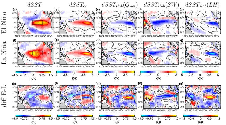
zonally wider during El Niño than during La Niña (Fig. 9a, f), resulting in a difference with an insignificant positive pole in the east that is surrounded by a significant horseshoe-type pattern of opposite sign (Fig. 9k). To account for the skew- ness, i.e., the asymmetry in amplitude between El Niño and La Niña events, both patterns have been normalized by the respective dSST averaged over the Niño3.4 region (black box in Fig. 9a, f), which is + 1.17 K and − 0.89 K for El Niño and La Niña, respectively. The dSST_oc in the eastern Pacific is larger during La Niña than during El Niño and extends slightly more westward (Fig. 9b, g). The difference between El Niño and La Niña reveals that dSST_oc during El Niño is smaller in the western, northwestern and in the far eastern equatorial Pacific, and larger in the central equatorial Pacific (Fig. 9l). The differences in the eastern Pacific, however, are not significant.

The dSST_slab(Q_net) pattern derived from observations is similar in the two ENSO phases (Fig. 9c, h), but with dif- ferences in amplitude. The difference pattern reveals a tri- pole structure at the equator, with stronger dSST_slab(Q_net) damping over the far eastern and western equatorial Pacific during La Niña relative to El Niño and weaker damping in the central Pacific (Fig. 9m). Only the difference in the cen- tral Pacific is significant. The dSST_slab(SW) during El Niño affects a larger area and the center extends more eastward than during La Niña (Fig. 9d, i), resulting in a quite strong asymmetry with a dipole structure of the differences at the equator (Fig. 9n). The asymmetry in dSST_slab(SW) is mainly caused by the more eastward position and strengthening of the SW feedback during El Niño and more westward posi- tion and weakening during La Niña (dashed and dashed- dotted lines in Fig. 6d, respectively), as the MLD asymmetry

120E 150E 180 150W 120W 90W

longitude -30

-20 -10 0 10

Qnet feedback [W/m*m/K]

(a)

120E 150E 180 150W 120W 90W

longitude -30

-20 -10 0 10

Qnet feedback [W/m*m/K]

(b)

all months El Nino La Nina Spread all months obs

120E 150E 180 150W 120W 90W

longitude -30

-20 -10 0 10

Qnet feedback [W/m*m/K]

(c)

120E 150E 180 150W 120W 90W

longitude -30

-20 -10 0 10

SW feedback [W/m*m/K]

(d)

120E 150E 180 150W 120W 90W

longitude -30

-20 -10 0 10

SW feedback [W/m*m/K]

(e)

120E 150E 180 150W 120W 90W

longitude -30

-20 -10 0 10

SW feedback [W/m*m/K]

(f)

120E 150E 180 150W 120W 90W

longitude -20

-15 -10 -5 0 5 10

LH feedback [W/m*m/K]

(g)

120E 150E 180 150W 120W 90W

longitude -20

-15 -10 -5 0 5 10

LH feedback [W/m*m/K]

(h)

120E 150E 180 150W 120W 90W

longitude -20

-15 -10 -5 0 5 10

LH feedback [W/m*m/K]

(i)

120E 150E 180 150W 120W 90W

longitude -100

-80 -60 -40 -20 0

Mixed layer depth [m]

(j)

120E 150E 180 150W 120W 90W

longitude -100

-80 -60 -40 -20 0

Mixed layer depth [m]

(k)

120E 150E 180 150W 120W 90W

longitude -100

-80 -60 -40 -20 0

Mixed layer depth [m]

(l)

Fig. 6 Heat flux feedbacks and mean mixed layer depth along the equator (5° S–5° N), in a net heat flux regressed on SST in Niño3.4 region in observation/reanalysis data; b same as a but here for the STRONG sub-ensemble; c same as a but here for the WEAK sub- ensemble; d–f same as a–c but here for the shortwave radiation; g–i same as a–c but here for the latent heat flux feedback; j–l same as

a–c but here for mean equatorial mixed layer depth; The solid line mark the values for all months, the dashed line for El Niño months and dashed-dotted for La Niña months; the light gray area marks the spread between the different models for “all months” case; The dark gray solid line in the second and third column are the observed values for the “all months” case for comparison