Isotopic evidence for biogenic molecular hydrogen production in the Atlantic Ocean

www.biogeosciences.net/13/323/2016/

doi:10.5194/bg-13-323-2016

© Author(s) 2016. CC Attribution 3.0 License.

Isotopic evidence for biogenic molecular hydrogen production in the Atlantic Ocean

S. Walter^1,a, A. Kock², T. Steinhoff², B. Fiedler², P. Fietzek^2,5, J. Kaiser³, M. Krol¹, M. E. Popa¹, Q. Chen⁴, T. Tanhua², and T. Röckmann¹

1Institute for Marine and Atmospheric Research (IMAU), Utrecht University, the Netherlands

2Marine Biogeochemistry, GEOMAR/Helmholtz-Centre for Ocean Research, Kiel, Germany

3Centre for Ocean and Atmospheric Sciences, School of Environmental Sciences, University of East Anglia, Norwich, NR4 7TJ, UK

4Department of Atmospheric Sciences, University of Washington, Seattle, Washington, USA

5Kongsberg Maritime Contros GmbH, Kiel, Germany

anow at: Energy research Center of the Netherlands (ECN), Petten, the Netherlands Correspondence to: S. Walter (s.walter@uu.nl)

Received: 14 September 2015 – Published in Biogeosciences Discuss.: 8 October 2015 Revised: 20 December 2015 – Accepted: 27 December 2015 – Published: 15 January 2016

Abstract. Oceans are a net source of molecular hydrogen (H2) to the atmosphere. The production of marine H2is as- sumed to be mainly biological by N2 fixation, but photo- chemical pathways are also discussed. We present measure- ments of mole fraction and isotopic composition of dissolved and atmospheric H₂from the southern and northern Atlantic between 2008 and 2010. In total almost 400 samples were taken during 5 cruises along a transect between Punta Are- nas (Chile) and Bremerhaven (Germany), as well as at the coast of Mauritania.

The isotopic source signatures of dissolved H₂extracted from surface water are highly deuterium-depleted and cor- relate negatively with temperature, showing δD values of (−629±54) ‰ for water temperatures at (27±3)^◦C and (−249±88) ‰ below (19±1)^◦C. The results for warmer water masses are consistent with the biological production of H2. This is the first time that marine H2excess has been di- rectly attributed to biological production by isotope measure- ments. However, the isotope values obtained in the colder water masses indicate that beside possible biological produc- tion, a significant different source should be considered.

The atmospheric measurements show distinct differences between both hemispheres as well as between seasons. Re- sults from the global chemistry transport model TM5 repro- duce the measured H₂mole fractions and isotopic composi- tion well. The climatological global oceanic emissions from

the GEMS database are in line with our data and previously published flux calculations. The good agreement between measurements and model results demonstrates that both the magnitude and the isotopic signature of the main components of the marine H₂cycle are in general adequately represented in current atmospheric models despite a proposed source dif- ferent from biological production or a substantial underesti- mation of nitrogen fixation by several authors.

1 Introduction

Molecular hydrogen (H2) is the second most abundant re- duced compound in the atmosphere after methane (CH4). H2

is not a radiatively active gas itself, but – via its role in at- mospheric chemistry – it indirectly influences the lifetime of the greenhouse gas CH₄and several air pollutants (Prather, 2003; Schultz et al., 2003; Tromp et al., 2003; Warwick et al., 2004; Jacobson, 2005, 2008; Feck et al., 2008; Ehhalt and Rohrer, 2009; Popa et al., 2015). The main H₂ sources are photo-oxidation of CH₄ and non-methane volatile organic compounds (NMVOCs) in the atmosphere and combustion processes at the surface, whereas soil deposition and oxida- tion by hydroxyl radicals (HO^•) are the main sinks. Oceans are a minor but significant source to the global H₂ budget with a mean estimated contribution of 7 %. However, esti-

mates of the oceanic contribution range from 1 to 15 % in different studies, indicating high uncertainties (Novelli et al., 1999; Hauglustaine and Ehhalt, 2002; Ehhalt and Rohrer, 2009; Pieterse et al., 2013 and references herein,).

Oceanic H₂production is assumed to be mainly biologi- cal, as a by-product of nitrogen (N₂) fixation (e.g., Conrad, 1988; Conrad and Seiler, 1988; Moore et al., 2009, 2014).

H₂is produced during N₂fixation in equimolar proportions, but also reused as an energy source. The H₂net production rate during N₂fixation depends on environmental conditions and also on microbial species (Bothe et al., 1980, 2010; Ta- magnini et al., 2007; Wilson et al. 2010a). Besides N2fix- ation, abiotic photochemical production from chromophoric dissolved organic matter (CDOM) and small organic com- pounds such as acetaldehyde or syringic acid has also been found to be a source of hydrogen in the oceans (Punshon and Moore, 2008a, and references therein).

Unfortunately, measurements that constrain the temporal and spatial patterns of oceanic H₂ emissions to the atmo- sphere are sparse. Vertical profiles display highest concen- trations in the surface layer (up to 3 nmol L⁻¹) and a sharp decrease with depth towards undersaturation, where the rea- sons for the undersaturation are not fully understood yet (e.g., Herr et al., 1981; Scranton et al., 1982; Conrad and Seiler, 1988). Tropical and subtropical surface waters are supersatu- rated up to 10 times or even more with respect to atmospheric H2equilibrium concentrations, and therefore a source of H2

to the atmosphere. This is in contrast to temperate and po- lar surface waters, which are generally undersaturated in H2

(Scranton et al., 1982; Herr et al., 1981, 1984; Herr, 1984;

Conrad and Seiler, 1988; Seiler and Schmidt, 1974; Lilley et al. 1982; Punshon et al., 2007; Moore et al., 2014).

Additional information to constrain the global H₂ budget and to gain insight into production pathways comes from the analysis of the H₂ isotopic composition (quantitatively expressed as isotope delta value,δD, see Sect. 2.2). Differ- ent sources produce H₂with characteristicδD values. More- over, the kinetic isotope fractionation in the two main re- moval processes, soil deposition and reaction with HO^•, is different. The combined action of sources and sinks leads to tropospheric H2with aδD of+130 ‰ relative to Vienna Standard Mean Ocean water (VSMOW), (Gerst and Quay, 2001; Rhee et al., 2006; Rice et al., 2010; Batenburg et al., 2011). In sharp contrast, surface emissions of H2from fos- sil fuel combustion and biomass burning haveδD values of approximately −200 and−300 ‰, respectively (Gerst and Quay, 2001; Rahn et al., 2002; Röckmann et al., 2010a;

Vollmer et al., 2010). As originally proposed by Gerst and Quay (2001), isotopic budget calculations require the pho- tochemical sources of H₂to be enriched in deuterium, with δD values between+100 and +200 ‰ (Rahn et al., 2003;

Röckmann et al., 2003; Feilberg et al., 2007; Nilsson et al., 2007, 2010; Pieterse et al., 2009; Röckmann et al., 2010b).

Biologically produced H₂has the most exceptional isotopic composition with δD of approximately−700 ‰ (Walter et

al., 2012), reflecting strong preference of biogenic sources for the lighter isotope¹H.

The aim of the study was (I) to determine theδD of dis- solved H₂and gain more information about possible sources, and (II) to get a high-resolution picture of the distribution of atmospheric H₂ along meridional Atlantic transects during different seasons and compare it with global model results.

Samples were taken on four cruises along meridional At- lantic transects in the Southern Hemisphere and the Northern Hemisphere and on one cruise at the coast of Mauritania. A total of almost 400 atmospheric and 22 ocean surface water samples were taken, covering two seasons between 2008 and 2010.

2 Methods 2.1 Cruise tracks

During four cruises of RV Polarstern and one of RV L’Atalante between February 2008 and May 2010, air and seawater samples were collected (see Fig. 1, Table 1). The cruises of RV Polarstern were part of the OceaNET project (autonomous measuring platforms for the regulation of sub- stances and energy exchange between ocean and atmosphere, Hanschmann et al., 2012).

They covered both hemispheres, between Punta Are- nas (Chile, 53^◦S/71^◦W) and Bremerhaven (Germany, 53^◦N/8^◦E). South–north transects were carried out in bo- real spring (April/May) and north–south transects in boreal autumn (October/November). The transects followed simi- lar tracks as the Atlantic Meridional Transect (AMT) pro- gramme (http://amt-uk.org/) and crossed a wide range of ecosystems and oceanic regimes, from sub–polar to tropical and from euphotic shelf seas and upwelling systems to olig- otrophic mid–ocean gyres (Robinson et al., 2009; Longhurst, 1998).

The RV L’Atalante followed a cruise track from Dakar (Senegal) to Mindelo (Cape Verde), covering a sampling area along the coast of Mauritania and a transect to the Cape Verde Islands. This area is characterized by strongly differ- ing hydrographical and biological properties with an inten- sive seasonal upwelling. Area and cruise track are described in more detail in Walter et al. (2013) and Kock et al. (2008).

2.2 Atmospheric air sampling

Discrete atmospheric air samples were taken on-board RV Polarstern at the bridge deck, using 1 L borosilicate glass flasks coated with black shrink-hose (NORMAG), with 2 Kel-F (PCTFE) O-ring sealed valves. The flasks were pre- conditioned by flushing with N₂at 50^◦C for at least 12 h;

the N₂ remained in the flask at ambient pressure until the sampling. During sampling the flasks were flushed for 4 min with ambient air at a flow rate of 12 L min⁻¹ using Teflon tubes and a membrane pump (KNF VERDER PM22874-

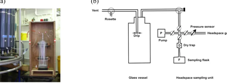
(a) (b)

Figure 1. (a) cruise tracks of the RV Polarstern, dots indicate positions of discrete atmospheric air sampling, (b) positions of surface water headspace sampling during ANT-XXVI/4 (n=16, green dots) and the RV L’Atalante ATA-3 cruise (n=6, black dots).

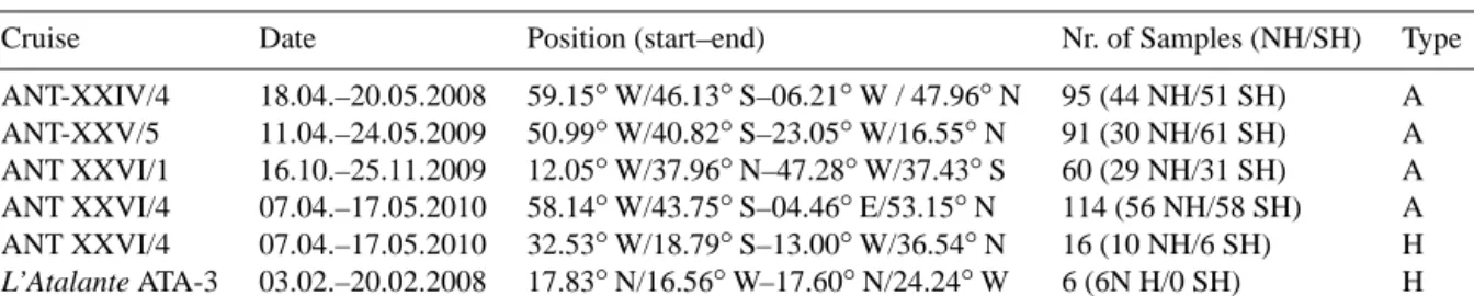
Table 1. Overview of sample distribution during the cruises: type A are discrete atmospheric samples, type H are headspace samples extracted from the surface water. The sample numbers in brackets give the number of measured samples in the Northern Hemisphere (NH) and Southern Hemisphere (SH).

Cruise Date Position (start–end) Nr. of Samples (NH/SH) Type

ANT-XXIV/4 18.04.–20.05.2008 59.15^◦W/46.13^◦S–06.21^◦W / 47.96^◦N 95 (44 NH/51 SH) A ANT-XXV/5 11.04.–24.05.2009 50.99^◦W/40.82^◦S–23.05^◦W/16.55^◦N 91 (30 NH/61 SH) A ANT XXVI/1 16.10.–25.11.2009 12.05^◦W/37.96^◦N–47.28^◦W/37.43^◦S 60 (29 NH/31 SH) A ANT XXVI/4 07.04.–17.05.2010 58.14^◦W/43.75^◦S–04.46^◦E/53.15^◦N 114 (56 NH/58 SH) A ANT XXVI/4 07.04.–17.05.2010 32.53^◦W/18.79^◦S–13.00^◦W/36.54^◦N 16 (10 NH/6 SH) H L’Atalante ATA-3 03.02.–20.02.2008 17.83^◦N/16.56^◦W–17.60^◦N/24.24^◦W 6 (6N H/0 SH) H

86 N86ANDC). The sample air was dried with Drierite^® (CaSO4). The flasks were finally pressurized to approxi- mately 1.7 bar, which allows duplicate measurements of the H₂isotopic composition of an air sample.

Table 1 gives an overview of the sampling scheme for dis- crete H₂samples. In total 360 samples were collected, reg- ularly distributed over the transects at 4 to 6 h intervals. In 2009 the resolution of sampling was enhanced to one sample per 2 h and focused on five sub-sections of the transect, in an attempt to resolve dial variability.

Samples were always taken at the downwind side of the ship to exclude a possible contamination by ship diesel ex- haust. One atmospheric sample was taken directly inside the ship’s funnel of RV Polarstern to determine the mole fraction and δD of ship diesel exhaust as a possible contamination source. This first measurements for ship diesel exhaust gave an H2mole fraction of (930.6±3.2) nmol mol⁻¹and aδD of

(−228.6±5.0) ‰. In the following, we will use the abbrevi- ation “ppb”=10⁻⁹in place of the SI unit “nmol mol⁻¹”.

2.3 Headspace sampling from surface waters

In addition to the atmospheric air samples, 16 headspace samples from surface water were taken during the RV Po- larstern cruise ANT-XXVI/4 in April/May 2010 and 6 sam- ples during the RV L’Atalante cruise in February 2008. The experimental setup (Fig. 2) was a prototype, and deployed for the first time to extract headspace air from surface water for isotopic composition measurements of molecular H₂. It consists of a glass vessel (10 L) and an evacuation/headspace sampling unit.

The glass vessel was evacuated for at least 24 h before sampling, using a Pfeiffer vacuum DUO 2.5A pump, with a capacity of 40 L min⁻¹(STP: 20^◦C and 1 bar). Water sam-

Figure 2. Experimental setup for headspace sampling, (a) sampling of the surface water into the glass vessel, connected to the Niskin bottle rosette, (b) scheme of the experimental setup.

ples were taken from 5 m depth (RV Polarstern cruises) or 10 m depth (RV L’Atalante cruise) using a 24-Niskin-bottle rosette with a volume of 12 L each. Sampling started imme- diately after return of the bottle rosette on-board and from a bottle dedicated to the H2 measurements. The evacuated glass vessel was connected to the Niskin bottle by Teflon tubing, which was first rinsed with approximately 1 L sur- face water. Then, 8.4 L water streamed into the evacuated flask (Fig. 2), using a drip to enhance the dispersion of the sample water. After connection of the headspace-sampling unit, the lines were first evacuated and then flushed with a makeup gas several times. During the RV L’Atalante cruise a synthetic air mixture with an H₂mixing ratio below thresh- old was used as makeup gas. The makeup gas used dur- ing the RV Polarstern cruises was a synthetic air mixture with an H₂ mole fraction of (543.9±0.3) ppb and aδD of (93.1±0.2) ‰. The mole fraction of the makeup gas was determined by the Max Planck Institute for Biogeochemistry and is given on the MPI2009 scale (Jordan and Steinberg, 2011). The glass vessel was pressurized to approximately 1.7 bar absolute with the makeup gas and the total headspace (added makeup gas plus extracted gas from the water sam- ple) was then flushed to a pre-evacuated sample flask. The flasks were of the same type as for the atmospheric sampling:

1 L borosilicate glass flasks (NORMAG), coated with black shrink-hose to minimize photochemical reactions inside and sealed with 2 Kel-F (PCTFE) O-ring sealed valves. All flasks were previously conditioned by flushing with N₂ at 50^◦C for at least 12 h and evacuated for at least 12 h directly be- fore use. The whole sampling procedure took around 15 min:

(4.0±0.5) min flushing surface water to the evacuated glass vessel, (8.0±1.0) min to connect the glass vessel to the sam- pling unit and evacuate the lines, and (3.0±0.5) min to add and pressurize the glass vessel with the makeup gas and take the headspace sample. The surface water temperature was on

average (0.9±0.6)^◦C higher than the air temperature. Given that most of the apparatus was at air temperature and that the headspace will adjust to ambient temperature relatively quickly during equilibration the air temperature was used for calculations. Since the temperature dependence of H2solu- bility is less than 0.3 % per K for seawater between 16 and 30^◦C (as encountered here) and view of the large H₂satura- tions (see below), the error associated with this assumption is negligible. Flasks were stored in the dark until measure- ment. Additionally, atmospheric samples were taken at the same location of headspace sampling (Table 4).

2.4 Measurements

2.4.1 Atmospheric H₂andδD (H₂) in discrete samples The mole fraction and isotopic composition of molecular H₂ was determined using the experimental setup developed by Rhee et al. (2004) and described in detail in Walter et al. (2012, 2013) and Batenburg et al. (2011). The D/¹H mo- lar ratio in a sample,Rsample(D/H), is quantified as the rel- ative deviation from the D/¹H molar ratio in a standard, Rstandard(D/H), as isotope delta δD value, and reported in per mill (‰):

δD= Rsample(D/H)

Rstandard(D/H)−1. (1)

The isotopic standard is Vienna Standard Mean Ocean Wa- ter (VSMOW). H₂mole fractions are reported as mole frac- tions in nmol mol⁻¹, abbreviated ppb (10⁻⁹, parts per bil- lion) and linked to the MPI2009 calibration scale for atmo- spheric hydrogen (Jordan and Steinberg, 2011). As work- ing standards, atmospheric air from laboratory reference air cylinders and synthetic air mixtures were used (Walter et al., 2012, 2013; Batenburg et al., 2011); the H₂ mole frac- tions of the air in these cylinders were determined by the

Max Planck Institute for Biogeochemistry, Jena, Germany.

The atmospheric reference air and the synthetic isotope ref- erence air were measured daily (atmospheric reference air at least twice) and results were used for correction of the sample measurements. The uncertainties reported here reflect random (i.e., repeatability) errors only and do not include possible systematic errors (Batenburg et al., 2011; Walter et al., 2012, 2013). Samples were measured in random order and analyzed within 3 months (ANT-XXIV/4, ANT-XXV/5, ANT-XXVI/1) up to 2 years (ANT-XXVI/4) after sampling.

Storage tests indicate that glass flasks equipped with Kel-F valves are stable for H2 (Jordan and Steinberg, 2011). The mean measurement repeatability between the two measure- ments on the same flask was between ±3.2 (ANT-XXV/5, n=14) and±6.4 ppb (ANT-XXVI/4,n=108) for the mole fraction and ±3.4 ‰ (ANT-XXVI/4, n=108) and±5.0 ‰ (ANT-XXV/5,n=14) for the isotopic composition.

H₂ and CO mole fractions were also measured by using a Peak Performer 1 RGA (Reduced Gas Analyzer) with syn- thetic air as a carrier gas, either continuously on-board (ANT- XXVI/4, see Sect. 2.4.2) or from discrete flasks in the labo- ratory (ANT-XXV/5 and ANT-XXVI/1). The discrete RGA measurements were performed from the same glass flasks after measurement of the isotope system (see above). Due to a remaining slight overpressure in the flasks, an active pumping of the air into the RGA was not necessary and the flasks were simply connected to the RGA inlet by Teflon tubing. The remaining pressure was mostly sufficient to per- form 8 to 10 measurements. A slight memory effect was ob- served and thus only the last 5 measurements were taken into account when stable. Samples with only three or less valid measurements were not used for evaluation. The stan- dards were the same as those used for the isotope system.

For both cruises (ANT-XXV/5 and ANT-XXVI/1), the mean measurement repeatability was better than ±0.8 (H₂) and

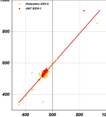
±2 % (CO). A comparison between the H₂ mole fractions measured with the Peak Performer 1 RGA and the isotopic experimental setup reveals on average slightly lower RGA values of (7.5±23.8) ppb (see Fig. 3).

2.4.2 Atmospheric H₂measured continuously

For the on-board continuous measurements of H2mole frac- tions a Peak Performer 1 RGA was used. The atmospheric air was drawn from the bridge deck to the laboratory in 1/4 inch Decabon tubing. The CO mole fraction was also measured in the same measurement and will be reported here for infor- mation, but without further discussion.

In alternating order, 10 air samples and 10 aliquots of ref- erence air were measured, using synthetic air as carrier gas.

Due to small memory effects, only the last 5 measurements of each were taken into account when the values were stable.

The mole fractions of H₂and CO were calculated by using the mean of the enclosing standard measurements, with an estimated maximal error of±5 %. For more details see Popa

Figure 3. Comparing the H₂mole fractions (ppb) measured with the isotopic experimental setup (x axis) and the Peak Performer 1 RGA (yaxis) during ANT-XXVI/1 (red labeled) and ANT-XXV/5 (yellow labeled),y=0.979x+3.96,R²=0.81,n=147.

et al. (2014). The mean measurement repeatability for the air samples was±1.7 % for H2and±3.6 % for CO in ambient air, respectively±0.8 (H₂) and ±0.9 % (CO) for the refer- ence air. Comparing the H₂mole fractions measured contin- uously on the RGA with discrete samples measured on the isotope system and collected close in time, we found a mean offset of (−18.8±16.4) ppb for the RGA results.

2.4.3 Dissolved H2extracted from surface water The discrete samples of extracted dissolved H₂ were mea- sured as described for the discrete atmospheric samples in Sect. 2.4.1. Details about assumptions and calculations to de- termine dissolved H₂concentrations and isotope delta values and quantity symbols are given in detail in the Supplement.

We define the extraction efficiencyηas η= c_hV_h

c_w0V_w, (2)

whereVhandVware the volume of the headspace and the wa- ter fraction, andc_hthe concentration of H₂in the headspace.

The initial concentration of H₂in seawater,c_w0, can be cal- culated from

cw0=c_hV_h

ηV_w. (3)

The concentration in the headspace, c_h, was not measured directly, but can be derived from the measured H₂mole frac-

tion in the sampling flask. The sampling procedure following gas extraction under vacuum can be broken into three steps (see Methods section):

1. expansion of the headspace into the gas transfer system 2. addition of makeup gas

3. expansion of the headspace / makeup gas mixture into a sample flask.

As shown in the Appendix, the original concentration of H2in seawater (in nmol L⁻¹) can be calculated using the fol- lowing equation

ηc_w0= y_fh

1+_V^Vt

h

p_htm−p_h(H₂O)i

−y_mh 1+_V^Vt

h

p_htm−p_hi

V_wRT ,

(4) wherey_f is the dry mole fraction of the air in the flask and y_mthe mole fraction of the makeup gas=(543.9±0.3) ppb.

The extraction efficiency,ηcan be calculated from the fol- lowing mass balance

Vwcw0=Vhch+αVwch. (5) Assuming that headspace gas phase and water phase are in equilibrium, the ratio of the H₂concentration in water and in the headspace is given by the Ostwald coefficient (Battino, 1984) (where the concentrations refer to in situ temperature):

α=c_w

c_h. (6)

This gives for the extraction efficiency as defined in Eq. (2) η=

1+αVw

Vh

−1

. (7)

In the present case, α=α(H2) was equal to 0.0163±0.0001, which gives η=92.12 (±0.013) % forVw/Vh=8.4/1.6=5.25.

Two alternative scenarios were considered to derive theδD of the dissolved H₂, with scenario 1 assuming equilibrium isotopic fractionation between headspace and water, and sce- nario 2 assuming kinetic isotopic fractionation during extrac- tion from Niskin bottle to glass vessel.

Scenario 1:δw0=δh+ε (1−η) (1+δh) (8) The equilibrium isotope fractionation between dissolved phase and gas phase isε=(37±1) ‰ at 20^◦C (Knox et al., 1992).

Scenario 2:δw0= (1+δ_h) η 1−(1−η)^1+εk

−1

≈δ_h+ε_k(1−η) (1+δ_h)ln(1−η)

η (9)

The kinetic isotope fractionation during gas evasion is ε_k=(−18±2) ‰ at 20^◦C (Knox et al., 1992). The approx- imation is not used and only shown to illustrate the small difference betweenδ_w0andδ_hwhenη≈1.

The temperature dependences ofεandεkare unknown and were neglected here.

The air saturation equilibrium concentration,csat(H₂), was determined using the parameterization of Wiesenburg and Guinasso (1979). The H₂ saturation anomaly, 1(H₂), was calculated as the difference between the measured H₂ con- centration,c(H₂), andc_sat(H₂):

1(H2)=c(H2)−csat(H2). (10) Meteorological and oceanographic parameters (radiation, air and water temperatures, salinity, relative humidity) were measured using standard instrumentation and recorded and provided by the data system of the ships. More information about devices and sensor documentation can be found on the website of the Alfred Wegener Institute http://dship.awi.de/.

Backward trajectories were calculated using the backward

“Hybrid Single Particle Lagrangian Integrated Trajectory”

(HYSPLIT, Schlitzer, 2012) model of the National Oceanic and Atmospheric Administration (NOAA, http://ready.arl.

noaa.gov/HYSPLIT.php).

2.5 Modeling 2.5.1 TM5 model

We performed simulations of H₂mole fractions and isotopic composition with the global chemistry transport model TM5 (Krol et al., 2005), and compared them with our measure- ment data (Fig. 5). The simulation setup was similar to the one of Pieterse et al. (2013) and only a short description is given here. The model version used employs the full hy- drogen isotopic scheme from Pieterse et al. (2009) and uses ERA-Interim meteorological data. The chemistry scheme is based on CBM-4 (Houweling et al., 1998), which has been extended to include the hydrogen isotopic scheme (that is, for all chemical species that include hydrogen atoms, HH and HD are treated separately and have different reaction rates).

The H₂ sources and isotopic signatures are given as input;

these and also the H₂soil deposition velocities are identical to Pieterse et al. (2013).

The model has a relatively coarse spatial resolution of 6^◦ longitude by 4^◦ latitude, and a time step of 45 min. Daily average mole fraction fields are used for comparison to ob- servations. The model results were interpolated to the time and location of the observations.

2.5.2 Global oceanic emissions

The climatological global oceanic emissions were calculated using the protocol of Pieterse et al. (2013), based on the GEMS database and an assumed mean oceanic H₂ source of 5 Tg a⁻¹ as given from global budget calculations (see Ehhalt and Rohrer, 2009, and references therein, Pieterse et al., 2013). The spatial and temporal variability of oceanic H₂ emissions caused by N₂ fixation are adopted from the spa-

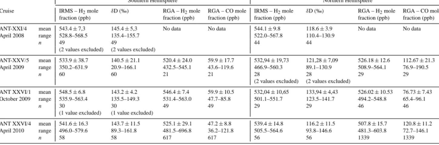
Table 2. Hemispheric means of atmospheric H₂and its isotopic composition along the four meridional Atlantic transects.

Southern Hemisphere Northern Hemisphere

Cruise IRMS – H₂mole δD (‰) RGA – H₂mole RGA – CO mole IRMS – H₂mole δD (‰) RGA – H₂mole RGA – CO mole

fraction (ppb) fraction (ppb) fraction (ppb) fraction (ppb) fraction (ppb) fraction (ppb)

ANT-XXI/4 mean 543.4±7,3 145.4±5,3 No data No data 544.1±9.8 118.6±3.9 No data No data

April 2008 range 528.8–568.5 135.4–155.7 522.0–567.8 110.4–130.9

n 49 49 44 44

(2 values excluded) (2 values excluded)

ANT-XXV/5 mean 533.9±38.7 140.5±21.1 520.4±24.0 59.9±17.7 532,94±19,73 121,28±7,09 526.18±12.6 112.67±21.3 April 2009 range 350.2–631.9 20.9–166.1 432.5–545.1 43.6–119.6 466.9–560.3 89.1–130.9 508.9–564.1 76.9–190.5

n 60 60 21 21 28 28 29 29

(2 values excluded) (2 values excluded)

ANT XXVI/1 mean 548.5±6.8 143.2±4.2 546.4±7.4 59.9±10.5 532,04±10,65 133,94±4,43 526.02±10.53 76.73±7.43 October 2009 range 535.9–563.4 135.5–149.3 531.4–563.0 47.7–85.8 501.1–551.7 123.5–141.7 494.2–548.8 65.4–96.1

n 30 30 49 49 29 29 46 46

(1 value excluded) (1 value excluded)

ANT XXVI/4 mean 541.6±16.3 143.7±11.5 525.1±29.1 47.2±8.8 539.4±14.8 116.2±11.5 507.8±15.7 120.8±11.2 April 2010 range 496.0–579.6 89.3–161.8 481.5–696.8 36.2–121.8 505.5–564.6 93.8–146.6 481.3–603.8 72.7–146.1

n 58 58 617 617 56 56 1339 1339

tial and temporal distribution of oceanic CO (Erickson and Taylor, 1992).

3 Results and discussion 3.1 Atmospheric H₂transects

Our data set includes data of two hemispheres and two sea- sons between 2008 and 2010 (see Table 2, Fig. 4). The mean mole fraction of H2 ranged between (532.0±10.7) and (548.5±6.8) ppb. In spring, the mean values were al- most equal between the hemispheres with approximately 1 to 2 ppb difference, but they differed significantly in au- tumn. In this season, the mean values in the Northern Hemi- sphere (NH) were approximately 16 ppb or 3 % lower com- pared to the Southern Hemisphere (SH), with a distinct tran- sition between the hemispheres at around 8^◦N. In contrast, δD differed significantly between the hemispheres in both seasons. In the Southern Hemisphere, absolute δD values were always between 9 and 27 ‰ higher than in the North- ern Hemisphere, and generally remained within a narrow range between (140.5±21.1) and (145.4±5.3) ‰. In con- trast to the mole fraction, isotope delta differences between the hemispheres were less pronounced in autumn than in spring. These two seasonal patterns, in the following defined as “summer signal” and “winter signal”, are mainly caused by biological processes and tropospheric photochemistry and driven by variations in the NH. They are in line with previ- ously published data and model results (Rhee et al., 2006;

Price et al., 2007; Rice et al., 2010; Pieterse et al., 2011, 2013; Batenburg et al., 2011; Yver et al., 2011; Yashiro et al., 2011).

The “summer signal”, observed in October, is character- ized by lower H₂mole fractions in the Northern Hemisphere and a less pronounced difference in δD between the hemi- spheres. Deposition by biological activity of microorganisms in the soils is the main sink of H₂ (Yonemura et al., 2000;

Pieterse et al., 2013) and the sink strength in the North- ern Hemisphere and the Southern Hemisphere depends on the distribution of landmasses and on season. With approxi- mately 70 % of landmasses in the NH and higher microbial activity in the summer, the mole fraction during this season is lower in the NH than in the SH. Due to the general pref- erence of organisms for molecules with lighter isotopic com- position, the δD values increase during summer in the NH and the interhemispheric gradient becomes less pronounced.

The “winter signal” observed in April is defined by al- most equal mole fractions and more pronounced differences inδD values between the hemispheres. In winter, molecu- lar hydrogen is accumulating in the NH hemisphere, and the main source is fossil fuel combustion with a depleted iso- topic composition of −170 to −270 ‰ (Gerst and Quay, 2001; Rahn et al., 2002). This leads to nearly equal mole fractions in both hemispheres and a more pronounced δD gradient, with isotopically lighter H2in the NH. The contri- bution of source and sink processes in the SH to the seasonal patterns is less pronounced than for the NH (Pieterse et al., 2011, 2013). As a result, the H₂ seasonal cycle in the SH is much weaker compared to the NH. The SH isotopic H₂ signature is caused by mainly emissions and chemical loss with an isotope delta of approximately+190 ‰, which ex- plains the generally higherδD values. The Intertropical Con- vergence Zone (ITCZ) separates the two hemispheres and is clearly visible, not only in the H₂distribution, but also in the CO distribution.

Simulations of H₂mole fractions and isotopic composition using the global chemistry transport model TM5 (Krol et al., 2005) compared with our atmospheric data reveal that the model simulates the H2mole fractions quite well (Fig. 5), with a slight overestimate of up to 20 ppb (which means up to 4 %).

The model results are less variable on small spatial scales, due to the low spatial resolution, and possibly to local influ- ences that are not included in the model (e.g., ocean emis-

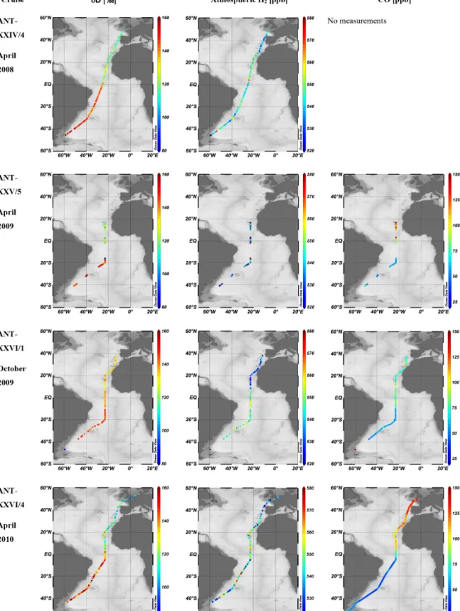
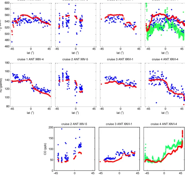
Figure 4.δD (H₂) (‰) (first column), H₂mole fraction (ppb) (second column), and CO mole fraction (ppb) (third column), along the meridional cruise tracks of RV Polarstern, the mole fraction andδD of H₂are measured by IRMS, the CO mole fraction by RGA.

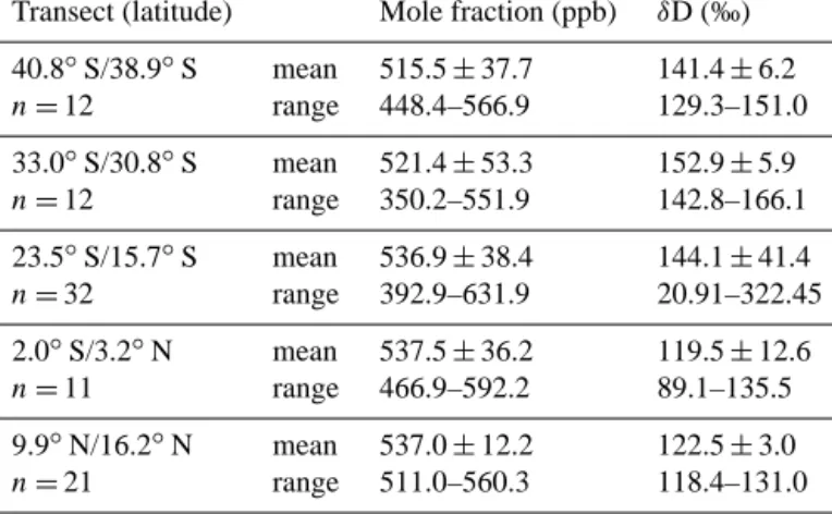
Table 3. Overview of means of atmospheric H₂ and its isotopic composition along the five high–resolution transects of ANT-XXV/5, including the standard deviation and the range.

Transect (latitude) Mole fraction (ppb) δD (‰) 40.8^◦S/38.9^◦S mean 515.5±37.7 141.4±6.2

n=12 range 448.4–566.9 129.3–151.0

33.0^◦S/30.8^◦S mean 521.4±53.3 152.9±5.9

n=12 range 350.2–551.9 142.8–166.1

23.5^◦S/15.7^◦S mean 536.9±38.4 144.1±41.4

n=32 range 392.9–631.9 20.91–322.45

2.0^◦S/3.2^◦N mean 537.5±36.2 119.5±12.6

n=11 range 466.9–592.2 89.1–135.5

9.9^◦N/16.2^◦N mean 537.0±12.2 122.5±3.0

n=21 range 511.0–560.3 118.4–131.0

sions in the model are less variable in time and space than they could be in reality). The largest differences between the modeled and measured H₂occur between 30^◦S and the equa- tor. This seems a systematic feature and could be due to a slight overestimation of sources or underestimation of sinks by the model. Despite these small differences, the model is consistent with measured H2 mole fractions and simu- lates them well. Large-scale features are clearly visible, like the sharp gradient around 10^◦N during cruise ANT-XXVI/1 (Fig. 5, top, third plot), or the decrease inδD towards north- ern mid-latitudes (most evident for the cruises ANT-XXIV/4 and ANT-XXVI/4, first and last plots in Fig. 5, top). A slight overestimate of the H₂ mole fractions was also noted by Pieterse et al. (2013). This might be explained by an overes- timate of photochemical sources in the model, which would influence only the mole fractions but not theδD values.

The model simulates the isotopic composition of H₂even better than the mole fractions. The most important features are the general decrease from south to north, and the sharp gradient around the equator. As most sources and sinks of H2 have very different isotopic signatures, this good com- parison indicates that the model adequately represents both the magnitude and the isotopic signature of the main compo- nents of the H₂cycle. Similar to Pieterse et al. (2013) we also observe a slight underestimate of theδD at high southern lat- itudes, which is possibly due to underestimating the isotopic composition assumed for H₂returning from the stratosphere in the latitude band 60 to 90^◦S.

3.2 Spatial and temporal high–resolution transects during ANT-XXV/5

In April 2009 the sampling resolution was increased to ap- proximately one sample per 2 h for five selected sections of the transect during ANT-XXV/5 (Fig. 4, Table 3): three in the Southern Hemisphere, one crossing the equator and one in the Northern Hemisphere. These transects were chosen based

on previously published data (Herr et al., 1984; Conrad and Seiler, 1988) and with the aim to get an indication of small- scale sources or diurnal cycles of atmospheric H₂for further investigations.

All transects showed neither a diurnal cycle nor a correla- tion with radiation and a range ofδD values within or only slightly outside a 2σ range around the mean, except for the one between 23.5 to 15.7^◦S (Fig. 6a). Here the highest H₂ mole fractions of (631.9±3.2) ppb, combined with the low- estδD values of (20.9±5.0) ‰, were found around 16^◦S.

Due to the limited spatial resolution and therefore low num- ber of data points, a Keeling plot analysis (Fig. 6b) of the data between 15 and 18^◦S was made with either 5, 7, or 9 data points to get a reasonable range for the source signature.

It reveals a mean source signature of−561.5 in a range of

−530 to−683 ‰ (n=7±2,R²=0.85±0.01). The corre- lation coefficient is a mean of the three analyses.

HYSPLIT trajectories for the samples collected on this transect during the 28 April 2010 and 1 May 2010 (21.8 to 15.7^◦S) reveal the same origin of air masses coming from the direction of Antarctica. Oceanographic parameters such as water temperature and salinity are similar and do not cor- relate with H₂mole fractions andδD values. These findings indicate a strong but local source, and the lowδD value for the source obtained by the Keeling plot analysis points to biological production (Walter et al., 2012). Such local and temporal patchiness of high H₂mole fractions in surface wa- ters was reported previously in correlation to high N₂ fixa- tion rates (Moore et al., 2009, 2014). Although reported for other oceanic regions, the H₂mole fractions andδD values here neither show a diurnal cycle (Herr et al., 1984), nor are they correlated with radiation indicating photochemical pro- duction (Walter et al., 2013), and most of the values were ob- served during night. Wilson et al. (2013) recently showed that H2production and uptake rates clearly depends on microbial species, and also on their individual day-night rhythm, but the contribution of different diazotrophs to the marine H2cy-

-45 0 45 0

50 100 150 200

lat (°)

CO (ppb)

cruise 2 ANT XXV-5

-45 0 45

lat (°) cruise 3 ANT XXVI-1

-45 0 45

lat (°) cruise 4 ANT XXVI-4

Figure 5. Comparison of measurement results of H₂and CO mole fractions andδD with TM5 model results (given in red). Data are shown against latitude. The blue markers show results of flask samples, and the green markers represent the continuous in situ measurements (performed with the peak performer instrument on–board). CO has not been analysed in the flasks sampled during the last cruise. The model data were interpolated at the place and time of sampling or measurements.

cle is unknown (e.g., Bothe et al., 2010; Schütz et al., 2004;

Wilson et al., 2010a, b; Punshon and Moore, 2008b; Scranton 1983, Moore et al., 2009).

Around 21.2^◦S one single sample with a low mole frac- tion of (393.9±3.2) ppb in combination with a highδD of (322.45±5) ‰ value was observed. As mentioned before HYSPLIT models reveal the same origin of air masses on this transect, thus this sample indicates probably a local sink.

However, this interpretation depends on only one single mea- surement point and although neither instrumental parameters indicated an outlier nor meteorological or oceanographical parameters differed from other samples, we cannot exclude an artefact due to sampling, storage, or analyses. A simple Rayleigh fractionation model reveals a fractionation factor

ofα=0.646±0.002, which is close to the value of oxida- tion by HO^• (α=0.58±0.07, Batenburg et al., 2011). An estimate of theδD value by using an HO^• oxidation frac- tionation factor would lead to an increase by 125 or 149 ‰, respectively. The observed increase ofδD seems reasonable when assuming oxidation by HO^•, but with respect to the HO^•mole fraction and the slow reaction rate of H₂+HO^•, it is questionable whether the H₂ decrease here can be ex- plained by this.

3.3 Dissolved H₂

A new method has been presented to extract H₂ from sur- face waters for isotopic determination. Before discussing the

(a) (b)

Figure 6. (a) H₂mole fraction (ppb) (black) andδD [‰ ] (red) along the ANT-XXV/5 high–resolution transect 24–15^◦S; (b) Keeling plot of the samples along the high–resolution transect north of 18^◦S. The three trend lines indicate the range of the Keeling plot analysis that was applied to determine the source signature.

measurement results, we will give an overview of the possi- ble main errors and their effects. To show the effect of the errors on the measurements, we will present error factors, thus how much the final data differ by shifting the respective parameter by 1 % and also the absolute assumed error.

For the extraction method several error sources could be identified: the determination of pressure, especially in the sampling vessel before adding the make-up gas and during extraction, the temperature of air and water, respectively the difference between them when the sample is extracted from the headspace, and the volume of the set-up and the sam- ple. The determination of pressure in the sampling vessel would be one issue of further improvement, because the er- ror caused by pressure deviations for the total pressure after adding the make-up gas is about a factor of 0.7 for concentra- tions and 0.2 for the isotopic values. The error based on tem- perature of air, water and sample is negligible due to high- precision measurements and the short handling time between water sampling and headspace extraction. The error for the volume parameter for the set-up is negligible due to the high volume, the precise determination of the glass vessel volume by weighing, and the calculation of the tubing volume. The main error source is the water volume of the sample, which counts by a factor of 5.9 for the concentration, but with neg- ligible effect on the isotopic values. Although the relative er- ror factor is quite high, the absolute value is assumed to be around 0.5 % due to the sample size, which has also been weighed at the home lab. The H2 measurement procedure is the same as for atmospheric samples and possible errors are described in the respective sessions or related literature.

However, the error caused by the determination of the dry mole fraction itself seems to have the main input by a factor of 5.3 for concentration and 4.6 for the isotopic values of dis- solved H₂. Errors of the determination of the isotopic value are much less significant and count by a factor of 0.2.

Taking measurement and handling errors during the ex- traction as well as errors in the determination of the dry mole fraction into account, we assume a robust overall uncertainty of±6.9 % for the dissolved H₂ mole fractions and±4.7 % for the isotopic values by calculating the root of the sum of the squared uncertainties.

As shown in Table 4 we also tested the effect of equilib- rium isotopic fractionation and kinetic isotopic fractionation.

The effect is less than 0.2 %.

Therefore, recommendations for the extraction method are to additionally measure parameters such as the initial pres- sure in the glass vessel and to ensure a precise determina- tion of the sample volume. Besides this we recommend high–

precision IRMS measurements and to consider multiple sam- pling for better statistics on the data.

3.3.1 H₂concentration

In total, 16 headspace samples were taken during the RV Polarstern cruise in April/May 2010 along the transect 32.53^◦W/18.79^◦S to 13.00^◦W/36.54^◦N and 6 samples dur- ing the RV L’Atalante cruise in February 2008 between 23.00–17.93^◦W to 16.9–19.2^◦N to analyze the H2 mole fraction and the isotopic composition (see Table 4).

Although our setup was a prototype with possibilities for improvement, the mole fractions are in line with previously published data. The H₂excess,1(H₂), exceeds 5 nmol L⁻¹, the saturation differ from close to equilibrium to 15-fold supersaturation. Highest supersaturation was found in the Southern Hemisphere between 16 and 11^◦S and in the Northern Hemisphere around the Cape Verde islands and the coast of Mauritania (Fig. 7a, Table 4).

Herr et al. (1984) reported patchy enhanced H₂concentra- tions in the surface water with up to 5-fold supersaturation in the subtropical south Atlantic (18–31 and 29–42^◦W). This is comparable to what Conrad and Seiler (1988) found in the

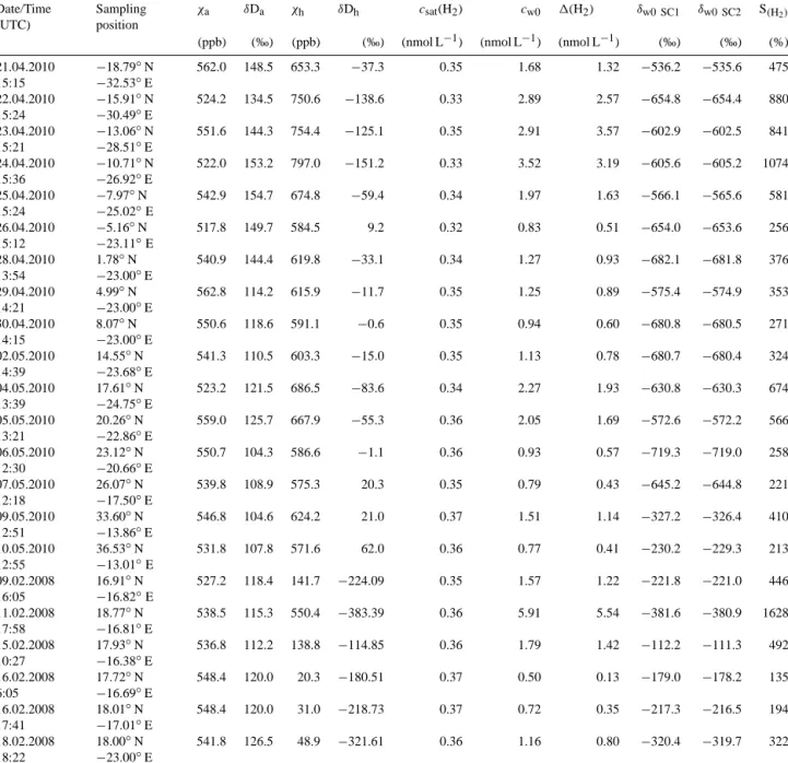
Table 4. Overview of headspace sample results from the ANT-XXVI/4 cruise (2010) and the L’Atalante ATA-3 (2008),:χ_his the measured mole fraction of the headspace in parts per billion (ppb=nmole mole⁻¹),χais the corresponding atmospheric mole fraction in ppb,δD_hand δD_ais the measured isotopic composition in permil (‰). The H₂equilibrium concentrationc_sat(H₂) was determined by using the equations from Wiesenburg and Guinasso (1979), the initial dissolved H₂concentrationc_w0is calculated as given in Supplement 1, and the excess 1H₂is the difference between them.δ_{w0 SC1}andδ_{w0 SC2}show the two scenarios to derive the initial isotope delta of dissolved H₂. S_(H2) is the saturation of H₂in the surface water. The calculated extraction efficiency was 92.12 (±0.013)%. The calculations are given in the Supplement in more detail.

Date/Time (UTC)

Sampling position

χ_a δDa χ_h δDh c_sat(H2) c_w0 1(H2) δ_{w0 SC1} δ_{w0 SC2} S(H₂)

(ppb) (‰) (ppb) (‰) (nmol L⁻¹) (nmol L⁻¹) (nmol L⁻¹) (‰) (‰) (%) 21.04.2010

15:15

−18.79^◦N

−32.53^◦E

562.0 148.5 653.3 −37.3 0.35 1.68 1.32 −536.2 −535.6 475

22.04.2010 15:24

−15.91^◦N

−30.49^◦E

524.2 134.5 750.6 −138.6 0.33 2.89 2.57 −654.8 −654.4 880

23.04.2010 15:21

−13.06^◦N

−28.51^◦E

551.6 144.3 754.4 −125.1 0.35 2.91 3.57 −602.9 −602.5 841

24.04.2010 15:36

−10.71^◦N

−26.92^◦E

522.0 153.2 797.0 −151.2 0.33 3.52 3.19 −605.6 −605.2 1074

25.04.2010 15:24

−7.97^◦N

−25.02^◦E

542.9 154.7 674.8 −59.4 0.34 1.97 1.63 −566.1 −565.6 581

26.04.2010 15:12

−5.16^◦N

−23.11^◦E

517.8 149.7 584.5 9.2 0.32 0.83 0.51 −654.0 −653.6 256

28.04.2010 13:54

1.78^◦N

−23.00^◦E

540.9 144.4 619.8 −33.1 0.34 1.27 0.93 −682.1 −681.8 376

29.04.2010 14:21

4.99^◦N

−23.00^◦E

562.8 114.2 615.9 −11.7 0.35 1.25 0.89 −575.4 −574.9 353

30.04.2010 14:15

8.07^◦N

−23.00^◦E

550.6 118.6 591.1 −0.6 0.35 0.94 0.60 −680.8 −680.5 271

02.05.2010 14:39

14.55^◦N

−23.68^◦E

541.3 110.5 603.3 −15.0 0.35 1.13 0.78 −680.7 −680.4 324

04.05.2010 13:39

17.61^◦N

−24.75^◦E

523.2 121.5 686.5 −83.6 0.34 2.27 1.93 −630.8 −630.3 674

05.05.2010 13:21

20.26^◦N

−22.86^◦E

559.0 125.7 667.9 −55.3 0.36 2.05 1.69 −572.6 −572.2 566

06.05.2010 12:30

23.12^◦N

−20.66^◦E

550.7 104.3 586.6 −1.1 0.36 0.93 0.57 −719.3 −719.0 258

07.05.2010 12:18

26.07^◦N

−17.50^◦E

539.8 108.9 575.3 20.3 0.35 0.79 0.43 −645.2 −644.8 221

09.05.2010 12:51

33.60^◦N

−13.86^◦E

546.8 104.6 624.2 21.0 0.37 1.51 1.14 −327.2 −326.4 410

10.05.2010 12:55

36.53^◦N

−13.01^◦E

531.8 107.8 571.6 62.0 0.36 0.77 0.41 −230.2 −229.3 213

09.02.2008 16:05

16.91^◦N

−16.82^◦E

527.2 118.4 141.7 −224.09 0.35 1.57 1.22 −221.8 −221.0 446

11.02.2008 17:58

18.77^◦N

−16.81^◦E

538.5 115.3 550.4 −383.39 0.36 5.91 5.54 −381.6 −380.9 1628

15.02.2008 10:27

17.93^◦N

−16.38^◦E

536.8 112.2 138.8 −114.85 0.36 1.79 1.42 −112.2 −111.3 492

16.02.2008 6:05

17.72^◦N

−16.69^◦E

548.4 120.0 20.3 −180.51 0.37 0.50 0.13 −179.0 −178.2 135

16.02.2008 17:41

18.01^◦N

−17.01^◦E

548.4 120.0 31.0 −218.73 0.37 0.72 0.35 −217.3 −216.5 194

18.02.2008 18:22

18.00^◦N

−23.00^◦E

541.8 126.5 48.9 −321.61 0.36 1.16 0.80 −320.4 −319.7 322

southern Atlantic, on a similar cruise track as the RV Po- larstern. Around the equator they measured H₂surface water concentrations up to 12-fold supersaturation. In the southern Pacific, Moore et al. (2009) combined H₂surface water mea- surements with N₂fixation measurements. They reported a strong correlation between these parameters, a patchy dis-

tribution and a steep maximum of H2 concentrations up to 12.6 nmol L⁻¹around 14^◦S.

The recently published data by Moore et al. (2014) show similar patterns across the Atlantic as we found, with highest values around the southern and northern subtropics. How- ever, our saturations are lower than the ones given by them, especially in the Northern Hemisphere. Such differences

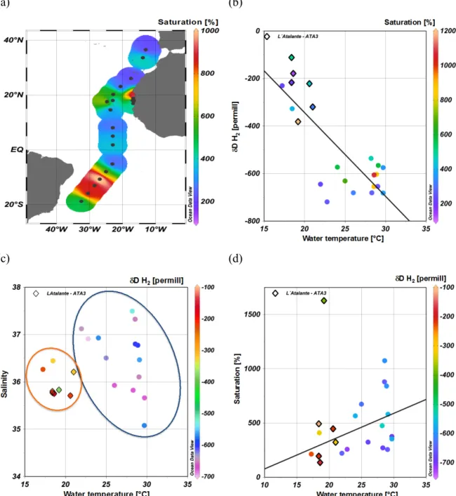
(a) (b)

(c) (d)

Figure 7. (a) H₂saturation in the surface water (color coded) along the RV Polarstern cruise track of ANT-XXVI/4 and the RV L’Atalante cruise ATA-3, with maxima around the Cape Verde islands and 10–15^◦S, Note: each sample is represented by a single dot. (b) Comparing theδD (H₂) at different water temperatures, the respective H₂saturation are color coded, sample dots marked with a diamond belong to the RV L’Atalante cruise, sample dots without to the ANT-XXVI/4 cruise;y= −35.2x+360.9,R²=0.66,n=22. (c) Distribution ofδD (H₂) (color coded) in correlation between water temperature and salinity. (d) Correlation between water temperature and H₂saturation, theδD (H₂) is color-coded, the exceptional high saturation has been excluded from the correlation calculation,y=0.26x−2.79,R²=0.22,n=21.

might be caused by experimental issues such as overesti- mated extraction efficiency or can be due to real temporal variability as the sampling seasons differed. The extraction efficiency has been estimated as 92.12 (±0.013) % (see Sup- plement) and was incorporated into the calculation of the original seawater concentration. With respect to the assump- tion of biological production as main production pathway it

is more likely that due to the different sampling seasons less H₂was produced in April than in October/November because of less microbial activity especially on the Northern Hemi- sphere in boreal winter.