Lecture # 4: Estimating Scoring Rules for Sequence Alignment
Scribe: Harel Shein 18/11/2008
1 Brief Review
In the previous lecture we discussed sequence alignment algorithms. Specifically we used the divide and conquer method to come up with a space efficient approach to sequence alignment. Finally we explained how our algorithm can be modified to enable local alignments.
2 Motivation
In our discussion of sequence alignment algorithms we assumed we have a given set of scoring rules for generating the alignment. Today we will discuss a way for generating these scoring rules. More specifically, cosidering weight functionsσ: Σ+×Σ+→ <
The choice ofσwill influence greatly the results. If we were to take evolution into account, what can we learn from it ?
Example 2.1 MalariaThe malaria genome is 80% AT, does this influence our decision ? Will an A-A match get the same score as G-G ? 40% of the genome is A or T and only 1-% is G or C, thus we must take the proir into account.
3 Decision making problem
3.1 Example
Let’s say I own an orchard (”Pardes”) and I would like to tell my orange sorting machine which oranges it should ship to Europe and which to Israel. I will try to rely on the color of the peel and decide if it’s a good orange. I have the following data:
If I want to find the threshold I need a decision rule:h:x→ −1,+1 Where x is the color, -1 is a bad orange and +1 is a good one.
Definition 3.1 α(h) =P−(x:h(x) = +1)
In words: the probability of objects I classified as good (+1) to be bad (-1).
And we will defineβ(h) =P+(x:h(x) =−1)
which is the probability of objects I classified as bad (-1) to be good (+1).
Definition 3.2 We say thath1dominatesh2ifh1is always better thath2, that is either:
• α(h1)< α(h2)∧β(h1)≤β(h2)Or:
• α(h1)≤α(h2)∧β(h1)< β(h2)
If the inequalities differ betweenαandβ, it’s harder to answer. We will therefore try to come up with a rule that tells us which is betterh1orh2.
3.2 Pareto Optimality
The boxed points represent feasible choices (decision rules), and smaller values ofαandβare preferred to larger ones. Point h3 is dominated by both point h1 and point h2. Points h1 and h2 are not strictly dominated by any other,
and hence lie on the curve. (This is called a Pareto Frontier, From Wikipedia:
http://en.wikipedia.org/wiki/P areto ef f iciency).
The following statistics lemma gives us an interesting result:
Lemma 3.3 (Neyman-Pearson) - h isundominatediff
∃ts.t. h(x) =sign(logPP+(x)
−(x)−t)where t is an offset.
The lemma states that the optimality line is defined by rules that follow this condition, meaning that you don’t need to look at other rules. We should use rules of the format of log ratio ofP+andP−.
4 Back to sequence alignment
We will now suggest aP+, P−model for the sequence alignment algoritm, in order to simplify our discussion we will assume the alignment is gap-less.
4.1 Building the model
Lets assume we can divide our analysis of the problem into two disjoint complimentary occurrences:
1. M - The sequences are evolutionarly relatedP(~x, ~y|M) 2. R - The sequences are unrelatedP(~x, ~y|R)
Lets consider the latter case first.
We will assume that the value of a given position is independent of adjacent positions in the sequence.
In addition, when the sequences are unrelated (R), we can assume that~x, ~y at any position are independent of each other (i.e.:∀i, P(xi, yi|R) =P(xi|R)P(yi|R)).1
In other words, for any position i, bothxiyiare sampled independently from some background distributionP0. So that the likelihood of the given~x, ~yto be unrelated is:
P(~x, ~y|R) =P(~x|R)P(~y|R) =
n
Y
i=1
P0(xi)P0(yi) (1)
In the first case above, we assume the two sequences are related, so they evolve from a common ancestor. For simplicity we will continue assuming that each position i in(xi, yi)is independent of the others. So we assumexi,yi
are sampled from some distributionP1of letter pairs. The probability that any two letters (”a”, ”b”) evolved from the same ancestral letter isp(a, b). So the likelihood of the given~x ~y, under this model is:
P(~x, ~y|M) =
n
Y
i=1
P1(xi, yi) (2)
4.2 A decision problem
So once again we have stumbled across a decision problem. Given the two sequences~x, ~ywe have to decide whether they are sampled from M (Model=related) or from R (Random=not related). We want to construct a decision procedure D(~x, ~y)that returns M or R. Basically we want to compare the likelihood of our data in both models.
First, lets notice that our decision procedure can make either one of two error types (same as before):
• Type I -~x, ~yare sampled from R butD(~x, ~y=M)
• Type II -~x, ~yare sampled from M butD(~x, ~y=R) The probabilities of such errors are also defined (also the same):
• α(D) =P(D(~x, ~y) =M|R)
• β(D) =P(D(~x, ~y) =R|M)
We would of course favor a procedure which minimizes both error types. Using the Neyman-Pearson lemma, let us look at the following equation:
P(~x, ~y|M) P(~x, ~y|R) =
Q
iP1(xi, yi) Q
iP0(xi)P0(yi) =Y
i
P1(xi, yi)
P0(xi)P0(yi) (3) Or for convenience, by taking a logarithm from both equation sides, of the form:
logP(~x, ~y|M) P(~x, ~y|R) = log
Q
iP1(xi, yi) Q
iP0(xi)P0(yi) =X
i
log P1(xi, yi)
P0(xi)P0(yi) (4) This expression tells us that we need to take the prior probabilities (P0) into account. Now we can define our scoring rule matrix as follows:
σ(a, b) = log P1(a, b) P0(a)P0(b)
1Why can we make this assumption? Every thing in biology tells us otherwise.
4.3 Parameter Estimation
If we could estimate the probabilitiesP1andP0from our data we would have our scoring matrixσ.
We will discuss parameter estimation through an example:
Let’s take the following i.i.d. samplesx1, x2, ..., xn ∼Pθwe would like to learn aboutPθ(X =x) =θxwhereθis a probability vector (θx≥0,P
xθx= 1).
Likelihood=`(~θ) =P(D|θ) =log(Y
i
Pθ(xi)) =X
i
log(Pθ(xi)) =(∗)X
x
Nxlogθx
* =Nx=P
i1{Xi =x}. That is,Nxis the number of times I sawxin the sample.
Definition 4.1 Sufficient Statistic :S(D)is a sufficient statistic if
S(D) =S(D0)⇒ ∀θPθ(D) =Pθ(D0).
In words, S keeps all the necessary information on the data to compute the likelihood. We’ll usually be interested in the minimal set of sufficient statistics.
We would like to generalize a process of finding an estimator. one method is the MLE - Maximum Likelihood Esti- mator.
4.4 MLE - Maximum Likelihood Estimator
We mark the estimatorθthat will maximizeL(θ), asθˆ= arg maxθ`(θ). To findθˆwe need to:
1. Calculate the likelihood function L.
2. Find a maximum for the likelihood function.
So how do we find the maximum of our likelihood function? By finding where∂θ∂` = 0.
In our example we’ll get:
∂`
∂θ = ∂
∂θx
X
x
Nxlogθx= Nx
θx
=!0⇒???
We have reched a dead end, we can’t concludeθˆfrom this equation. This brings us to the development of a Lagrangian.
4.5 Langrange Multipliers (aka Coefficients)
When we have a problem of optimization off(x)but we have some constraint C(x) = 0, we will define a new Lagrangian function
J(x, λ) =f(x)−λc(x)
and we will want to show that when the partial derivative ofxandλis zero - the constraint is satisfied and we are in stationary point. This means we solved the original problem.
When we take a partial derivative ofλ,
∂J
∂λ =C(x) =!0
and compare to zero, our constraint is satisfied and when we take a partial derivative ofx
∂J
∂x =∂f(x)
∂x −λ∂c(x)
∂x =!0⇒ ∂f(x)
∂x =λ∂c(x)
∂x we find the optimum.
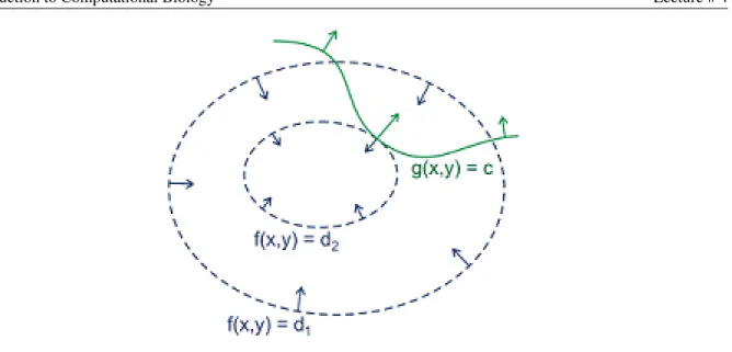
We showed that the derivation according toxoff(x)is a linear combination of the gradients of the constraints - we are in a point on the line of the constraint, where you can go no further, in the direction off(x)(if we are going on the line of the constraint as long as we go transversally to the contour line off(x)we are going ’uphill’, but when we touch it tangentially we can go no further - ’top of the hill’. We know we got to this point when the two derivatives are the same).
Figure 1: Drawn in green is the locus of points satisfying the constraint g(x, y) = c. Drawn in blue are con- tours of f. Arrows represent the gradient, which points in a direction normal to the contour.(from Wikipedia http://en.wikipedia.org/wiki/Lagrange multipliers)
4.6 back to MLE
θˆ= arg max
θ `(θ) where C (the constraint) is
X
x
θx−1 = 0
so we get
J(~θ, λ) =X
x
Nxlogθx−λ(X
x
θx−1)
taking the partial derivative usingθxwe get
∂J
∂θx =Nx
θx −λ=! 0 so we get
λ=Nx θx
⇒θx= Nx
λ (5)
taking the partial derivative usingλwe get
∂J
∂λ = 1−X
x
θx=!0⇒X
x
θx= 1 (6)
now, using results (5) and (6) we get X
x
Nx
λ = 1⇒λ=X
x
Nx
using (5) again we now conclude that
θx= Nx P
xNx
this result corresponds to our intuition about the likelihood of the data.