Investigations
on the Impact of Ions on the Air-Water-Interface
Dissertation
zur Erlangung des Doktorgrades der Naturwissenschaften (Dr. rer. nat.) der Naturwissenschaftlichen Fakult¨at IV - Chemie und Pharmazie
der Universit¨at Regensburg
vorgelegt von:
Eva Brandes
aus G¨ottingen
2019
Promotionsgesuch eingereicht am: 16. Mai 2019 Tag des Kolloquiums: 15. Juli 2019
Diese Arbeit wurde angeleitet von: Prof. Dr. Hubert Motschmann Pr¨ ufungsausschuss: Prof. Dr. Hubert Motschmann apl. Prof. Dr. Richard Buchner Prof. Dr. Arno Pfitzner
Vorsitzender Prof. Dr. Robert Wolf
Danksagung
Diese Doktorarbeit entstand am Institut f¨ ur Physikalische und Theoretische Chemie der Universit¨at Regensburg. Ohne die Zusammenarbeit und dem Austausch mit einer Reihe von Menschen w¨are dies nicht m¨oglich gewesen.
Zuallererst m¨ochte ich mich bei Hubert Motschmann bedanken. Er hat mich herzlich in seine kleine aber feine Arbeitsgruppe aufgenommen und mich in die faszinierende Welt der Grenzfl¨achenspektroskopie entf¨ uhrt. Zudem hat er mir erm¨oglicht, an zahlreichen Konferenzen teilzunehmen, somit konnte immer auch ein bisschen ¨ uber den Tellerrand hinauszugucken.
Besonderer Dank gilt auch Peter Karagiogiev, er hat mich mit großer Geduld in die technische Welt der Laserspektroskopie eingef¨ uhrt und stand mir immer mit Rat und Tat zur Seite.
Im Rahmen dieser Arbeit habe ich die M¨oglichkeit bekommen, hochinteressante Messungen mit Hilfe der Dielektrischen Relaxationsspektroskopie durchf¨ uhren zu k¨onnen. Ich m¨ochte Richard Buchner daf¨ ur danken, dass er mir diese Messungen erm¨oglicht hat und mir bei der Interpretation der Daten sehr geholfen hat. Ohne die Hilfe von Andreas Nazet w¨are mir die technische Durchf¨ uhrung nicht m¨oglich gewesen.
F¨ ur die Zusammenarbeit an dem Katalyse-System m¨ochte ich Stefan Tropp- man, Antonin (Tonda) Kralik und Burkhard K¨onig danken. Sie haben mir dieses interessante System vorgestellt und die Proben daf¨ ur synthetisiert.
Ich m¨ochte allen Mitgliedern des Lehrstuhles Kunz danken, insbesondere meinen Arbeitsgruppenkollegen Christian Luigs, Matthias Hofmann, Alexander Dietz, Ulrike Paap und Dominik Feucht. Es war immer m¨oglich einen Ansprechpartner f¨ ur Fragen und Hilfestellungen zu finden.
F¨ ur die sch¨onen Mittagspausen m¨ochte ich vor allem Beate M¨oser, Christoph
H¨olzl, Ragnhei
kur (Hei
ka) Gu
kbrandsd´ottir und Philipp Dullinger danken. Neben
den Mittagspausen entwickelte sich die Spieleabende zu einem fast w¨ochentlichen
deren Brettspiele die wir im Laufe der Jahre spielten.
Ein besonderer Dank gilt meinen Eltern und insbesondere meinem Freund
Drewes, die mir immer den R¨ ucken freigehalten haben und mich bei allen meinen
T¨atigkeiten immer unterst¨ utzt haben.
Contents
1. Introduction
. . . . 1
2. Theory
. . . . 3
2.1. Ion Specificity . . . . 3
2.1.1. Structure Maker and Structure Breaker . . . . 4
2.1.2. Law of Matching Water Affinities . . . . 4
2.2. Theories on the Ion Distribution at Interfaces . . . . 5
2.2.1. Charged Interfaces . . . . 6
2.2.2. Ion Specificity at Air-Electrolyte Interfaces . . . . 8
2.2.3. Experimental Data and its Implications . . . . 11
2.3. Polarization and Dielectric Relaxation . . . . 15
2.4. Light and its Theories . . . . 17
2.4.1. Definitions . . . . 17
2.4.2. Snell’s Law . . . . 19
2.4.3. Brewster Angle . . . . 19
2.4.4. Limit of Diffraction . . . . 21
3. Methods
. . . . 23
3.1. Sum Frequency Generation Spectroscopy . . . . 24
3.1.1. Theoretical Foundations of SFG . . . . 24
3.1.2. Selection Rules of SFG . . . . 28
3.1.3. Signal Intensity . . . . 30
3.1.4. Spectral Regions . . . . 31
3.1.5. Technical Description of the Device . . . . 34
3.1.6. Probe Preparation . . . . 39
3.1.7. Measuring Routine . . . . 40
3.1.8. Fitting Mechanism . . . . 41
3.2.2. Solvation Processes . . . . 45
3.2.3. Ion Pairs . . . . 47
3.2.4. Instrumentation . . . . 48
3.3. Supplementary Methods . . . . 49
3.3.1. Ring Tensiometer . . . . 49
3.3.2. Langmuir Trough . . . . 50
3.3.3. Brewster Angle Microscope . . . . 52
3.3.4. Lunkenheimer Surface Purification . . . . 53
3.3.5. NMR . . . . 54
3.3.6. Ellipsometry . . . . 55
3.3.7. SHG . . . . 56
3.3.8. MD-Simulation . . . . 56
4. Octahedral Complexes
. . . . 59
4.1. Introduction to the System . . . . 59
4.2. Sample Preparation . . . . 59
4.3. Hexacyanoferrate (HCF) . . . . 60
4.3.1. SFG Measurements on
HCF. . . . 60
4.3.2. DRS Measurements on
HCF. . . . 62
4.3.3. Comparison of DRS Data with SFG Data . . . . 66
4.4. Hexacyanocobaltate (HCC) . . . . 67
4.4.1. SFG Measurements on
HCC. . . . 67
4.5. Comparison of
HCFand
HCC. . . . 69
5. Catalysis on Membranes
. . . . 73
5.1. Scientific Issue . . . . 73
5.2. Description of the System . . . . 74
5.3. Comparison of Different Phospholipids . . . . 77
5.3.1. Impact of the Phospholipid . . . . 77
5.3.2. Impact of the Subphase . . . . 81
5.4. Deuterated Phospholipids . . . . 85
6. Lipid Ion Pairing
. . . . 89
6.1. Preliminary Work . . . . 89
6.1.1. SHG . . . . 90
6.1.2. Ellipsometry . . . . 90
6.1.3. MD-Simulation . . . . 93
6.2. Measurements on
C12-DMP-Br. . . . 94
6.2.1. Evaluation of the Purity of the Probe . . . . 94
6.2.2. SFG Investigation of the System . . . . 95
6.2.3. Interpretation of the Data . . . . 97
7. Concluding Remarks
. . . 101
A. Appendix. . . . I
A.1. Character Tables . . . . II
A.2. Symmetry Reduction . . . . V
A.3. Chemicals . . . VII
A.4. Devices . . . . IX
List of Figures. . . . XI
List of Tables. . . XV
Bibliography. . . XVII
1 Introduction
Water covers over seventy percent of the earth, most of it is salt water stored in the oceans. Additionally to the surface water, a large amount of water is located in the atmosphere, where it governs not only the weather, but is as well one major source of the natural greenhouse effect.
1Water is a quite peculiar liquid; it is famous for its density anomaly and its extended hydrogen bond network. Additionally to the exceptional bulk behavior there occur some surprising effects at the surface, too. These effects play little role for e.g. sea water, which acts in most cases as a more or less homogeneous bulk. However, in the atmosphere, surface effects of water droplets become more dominant. This is due to the high surface to bulk ratio of the droplets. Addi- tionally, surfaces are the predominant feature of all reactions in inhomogeneous systems. Therefore, it is worth to take a closer look at the water surface in various instances.
Interfaces are hard to investigate. This is the reason why many effects are still under discussion or yet wait to be discovered. Interfaces make up only a tiny fraction of the system and have a quite small geometrical extension. Never- theless, they are frequently the site of reactions and phenomena that dominate the macroscopic properties of the entire system. Hence, the understanding of the self-organization of molecules at interfaces is a central theme of colloid and interface science.
Linear and nonlinear optical reflection techniques are powerful tools in the armory of surface scientists that deepened our understanding of the interfacial architecture. In the recent years the picture of the air-water interface was altered, especially the non-monotonic concentration profile of ions was introduced as a new concept. It shows that the interface should be rather termed as interphase , because it has a vertical extension and is far more than just a dividing surface.
To investigate the air-water interface I used a surface specific spectroscopy –
namely SFG spectroscopy. Not the pure air-water interface was in focus, but rather the structural changes of the interface upon the modification with a salt, or with a membrane. The pure air-water interface shows already many interesting features, however, the presence of other substances proved to have great impact on the interfacial water. I investigated both, the impact of the interface on the probe and vice versa. This was accomplished by the simultaneously observation of the resonances of the probe itself and of the interfacial water. Additionally, I paid special attention to the effect of the counterions. Counterion binding is known to have a great impact on the interfacial structure.
In this thesis three systems were investigated. The pure electrolyte-air interface
of two octahedral metal complexes showed some interesting features, which could
be correlated to the bulk structure (section 4). A photoelectric catalytic system
was investigated, and structural effects proved to be an important factor for
the optimization of the reaction (section 5). In the third part the concentration
dependent counterion pairing of a charged amphiphile could be described (section
6). All of these very different systems showed interesting features in the interfacial
region.
2 Theory
In this chapter the most important theoretic concepts used in this thesis are presented. Liquids in general and liquid surfaces in particular are a complex sys- tem with many possible approaches for the theoretical description. The schemes shown in the following give a first insight in the general structure of water and electrolytes and then introduce basic theories of light matter interaction. The latter is the basis for the methods introduced in chapter 3.
2.1. Ion Specificity
Ions are in the most simple approach (see section 2.2) described as point charges with only electrostatic interaction with the surrounding. This picture is far too simple and does not capture the variety of ion phenomena. Especially the polar- izability and the solvation shell of ions leads to ion specific behavior. The first experimental data on this topic were produced by Franz Hofmeister in 1888. He studied the denaturation of proteins using dissolved egg white by adding salt.
The experiments revealed a dependence on the nature of the salt, which can-
not be explained models assuming only point charges.
2Hofmeister introduced
an order for both, anions and cations, which is well known as the Hofmeister or
lyotropic series . He noted that the monitored effects are most likely based on
a series of interactions such as lyotropic swelling of proteins, water binding or
osmotic pressure.
3Although this series was developed on proteins it turned out
that the order of the ions appear in various contexts. Some examples are shown in
section 2.2.3. Since the publication of Hofmeister there have been many efforts to
give a physical description of the ion specificity. The more research on the topic
was carried out, the more questions arose. For example in the investigations of
Klobusitzsky from 1925 some anions change place when changing the cation from
potassium to sodium.
4This indicates a strong impact of the counter ion on the
structure, anions and cations cannot be described separately. Even until this day there is no unifying theory of the Hofmeister effects, the Holy Grail of solution chemistry.
52.1.1. Structure Maker and Structure Breaker
It is undeniable that the impact of the ions on water is one of the major causes of the Hofmeister effects. Depending on the nature of the ion, the induced structure may vary. Small ions have a higher charge density than large ones of the same charge. The key idea is to put the ion-ion interaction in relation to the ion-water interaction. Small ions have a large impact on the surrounding water even beyond the first hydration shell. These ions are called structure maker.
6Large ions are termed as structure breaker.
7Very similar to these expressions are the terms kosmotropic and chaotropic, which were introduced by Collins and Washbough in 1985.
82.1.2. Law of Matching Water Affinities
Collins predicted the formation of contact ion pairs depending on the competitive interactions of the ions with their counterions and with water. This concept is referred to as the law of matching water affinities. Hard ions have a very strong interaction with other hard ions. A little bit less strong is the interaction of hard ions with water. For soft ions this relationship is the other way round, they experience stronger interactions with water than with other soft counterions. The water-water interaction is somewhere in the middle of these two extremes. Two hard ions will prefer the direct interaction, instead of being solvated by water.
When there are only soft ions in the solution, the predominant interaction is between the water molecules. They bind more likely to themselves than solvating the soft ions, which form as a consequence ion pairs. Only in a mixture of soft and hard anions and cations the ions will be separated from each other. This prediction seems to correlate with experimental data. For example the solubility of alkali halides experiences a minimum at matching water affinities (see table 2.1). However, in this model solvent separated ion pairs cannot be described (see section 3.2.3).
One example for ion pairing affects the taste of coffee. One major component
of coffee responsible for the bitter taste is caffeine, which is mainly known for
2.2. Theories on the Ion Distribution at Interfaces [mol/L] F
−Cl
−Br
−I
−Li
+ 0.119.6 20.4 8.8 Na
+1.0 6.2 8.8 11.9
K
+15.9
4.87.6 8.7 Rb
+12.5 7.5 6.7 7.2 Cs
+24.2 11.0
5.1 3.0Table 2.1.: Solubility of different alkali halides.9 The lowest solubility of each anion is marked in bold.
its stimulating properties. Caffeine tends to form to a certain extent dimers.
Other than the monomers, the dimers are not bitter.
10The extent of dimeriza- tion strongly depends on other additives in the solution, such as salts or sugar.
Kosmotropes tend to lead to dimerized caffeine, while more monomers form upon the addition of chaotropes.
11There are some recent measurements on the system suggesting that this effect results from competitive binding. Caffeine prefers to bind to added chaotropes instead of forming dimers. On the other hand, kos- motropes are excluded from the caffeine vicinity, leading to a dimerization of the caffeine. The highly hydrated sucrose acts as a kosmotrope. The less bitter taste of sweetened coffee is therefore not only pure imagination, but rather a result from the dimerization of caffeine.
122.2. Theories on the Ion Distribution at Interfaces
The description of ion distributions at charged or non-charged interfaces evoke a series of theories and improvements of the theories in the past. Some are based on first principles, some use a variety of fit parameters, but all of them try to solve the puzzling question of ion behavior close to the interface. In this section I want to give a historic overview over the zoo of theories. First these theories were proposed for the case of a charged metal surface exposed to the electrolyte.
This picture was modified also for other system such as a charged amphiphile at the air-electrolyte interface.
The electrostatic interaction of dissolved ions with the solvation molecules gets
usually described by the Poisson Boltzmann equation. Here the ions are treated
as point charges and only the interaction between ions and the influence of the
thermal motion is captured. Interactions of ions are calculated relative to the
mean field instead of individual interactions. This approach gives reasonable re- sults for concentrations smaller than 200 mM and potentials lower than 50 mV.
132.2.1. Charged Interfaces
There are several models trying to describe the electrostatic structure at charged interfaces. In figure 2.1 an overview over the different double layer models is given, which will be discussed in the following.
Helmholtz layer
Helmholtz
d
diffuse layer
Gouy-Chapman
d
Stern
diffuse layer Helmholtz
layer
d
Grahame
diffuse layer Helmholtz
layer
d
Figure 2.1.: Comparison of the ion distribution and the electric potentialϕ for dif- ferent double layer models (for details see text).
2.2. Theories on the Ion Distribution at Interfaces
Helmholtz Double Layer
Hermann von Helmholtz was the first one to tackle the ion distribution at a charged interface. He introduced the term electric double layer.
14His approach is, similar to many early concepts, based purely on electrostatic. He predicted a single counter ion layer adjacent to the charged surface. In this oversimplification thermal motion, ion diffusion, adsorption onto the surface and solvent-surface interaction are considered negligible. The resulting electric potential
ϕdecreases in a linear fashion from the charged interface to the liquid bulk value.
Gouy-Chapman Double Layer
The static picture introduced by Helmholtz was improved by Louis Georges Gouy and David Leonard Chapman independently in separate publications in 1910
15and 1913
16, respectively. Instead of fixed point charges the ions are subject to Brownian motion. No Helmholtz layer is formed, and the ion concentration decays exponentially. The extension of the diffuse layer is far reaching into the liquid. With this approach, Maxwell-Boltzmann statistics can be applied. The great drawback of this theory is the negligence of spatial extension of the ions, which allow unrealistic high ion concentrations at the interface. However, for very small concentrations in the range below one millimolar, this model gives reasonable results.
Stern Layer
To overcome the limited concentration range of previous approaches, Otto Stern
combined in 1924 the static layer of Helmholtz with the diffuse concentration
profile of the Gouy-Chapman theory.
17Some ions are specifically adsorbed to
the interface and form the so-called Stern layer. The finite size of ions is taken
into account, which limits the closest approach of an ion to the charged interface
by the ionic radius. The electric double layer is assumed to be thin compared
to the size of the particles. No Brownian motion is taken into account in this
layer. Major drawbacks of this method are the constant dielectric permittivity
and viscosity throughout the diffuse layer and disregard of all interactions other
than coulombic.
Grahame’s Modification
David C. Grahame altered the Stern model in 1947 in order to overcome some of the problems.
18He noted that the electrode is usually occupied by solvent molecules. The ions would have to lose its solvation shell allowing them to get in contact with the charged surface. He divided the Helmholtz layer in an inner and an outer part, where the inner plane is defined via the radius of the adsorbed solvent molecules and the outer plane by the distance of the center of the ions at the closest approach to the electrode. These layers are followed by the diffuse layer.
Other Non-Ionspecific Theories
After the basic setup many more approaches followed. The description was e.g.
altered by an introduction of a finite size of the ion, the dependence of the di- electric constant on the electric field, image forces or ion correlation.
19–22In all cases a combination of a static layer followed by a diffuse layer is used.
2.2.2. Ion Specificity at Air-Electrolyte Interfaces
At the air-electrolyte interface many ion specific effects can be observed. Ions are attracted by the interface by dipole - induced dipole interactions, and are at the meantime repulsed from the surface by electrostatic interactions. Depending on the nature of the ions, e.g. the polarizability, one or the other contribution dom- inates. In electrolyte solutions the electrostatic contribution is always strongly dependent on the counterion distribution. Furthermore, the interfacial water structure reorients upon addition of ions, which may alter the ion contribution.
The interaction of all these properties leads to a complex picture, where it is a difficult task to interpret experimental data in a meaningful manner.
With classical thermodynamics it is possible to describe equilibria at interfaces.
This is based on the Gibbs energy
Gwith the easily accessible variables pressure
pand temperature
T. If a surface is present, the surface tension
γand the surface area
Aare included. The differential of the Gibbs energy
dGis a function of the pressure, the temperature, the number of particles
niof the phase
iand of the surface area.
dG
=
V dp−SdT+
Xi
µidni
+
γdA(2.1)
2.2. Theories on the Ion Distribution at Interfaces
If the surface area is increased, the Gibbs energy change depends on the surface tension.
The surface tension is strongly dependent on the interfacial structure. It results from the cohesive force between molecules. In the bulk this cohesive force pulls the molecule isotropically in all directions. At the surface the lack of binding partners leads to an asymmetric picture (see figure 2.2). Since the attractive force pulls the molecules at the interface in the direction of the bulk, a defined surface is formed.
Figure 2.2.: Change in the coordination number upon pushing a molecule from the bulk to the surface and creating a new surface area.
The surface tension can be approximated with a simple approach. At constant pressure, temperature and particle number the surface tension only depends on the energy and the surface area. The energy can be estimated by the coordination number
ziand the corresponding binding energy
wAA. The change in area is just given by the area of the molecule (r
2, rough estimation via the radius). This assumes that the observed molecule pushes the molecules at the surface to the side and creating a new surface.
γ
=
∂G∂A
p,T,ni
≈
∆E
∆A
≈ wAA2
zB−zS
r2
(2.2)
The coordination numbers of the bulk are usually larger than at the surface. The binding energy can be estimated by the enthalpy of vaporization ∆H
vap. For simple molecules, such as
CCl4this estimation gives reasonable values.
In the systems investigated in this thesis, this approach is too simple. Gibbs
introduced the quantity of the surface excess Γ
i=
nAi, where the number of moles
of component
niis set in relation to the interfacial area
A. The total differentialof the surface tension
γis now only dependent on the surface excess and the chemical potential
µi.
−dγ
=
Xi
Γ
iµi(2.3)
One of these components is the solvent, others are in the case of a univalent salt the anion, the cation and the undissociated salt. The Gibbs dividing surface is chosen such that the term of the solvent vanishes.
23With the definition of the chemical potential it is possible to derive the Gibbs adsorption isotherm.
−dγ
=
mRTΓ
2dln
a1(2.4)
≈mRT
Γ
2dln
c1(2.5)
For dilute solutions the activity
a1can be replaced by the concentration
c1. The coefficient
mtakes the dissociation into account. For a univalent ion the extrema are
m= 2 for a completely dissociated salt and
m= 1 for an undissociated salt.
24For partially dissociated salts the value is in between.
25The surface excess is the excess of the surface concentration over the bulk concentration. A common representation is a plot of the surface tension versus the logarithm of the concentration.
Γ
2=
−1
mRTdγ d
ln
ai(2.6)
≈ −
1
mRTdγ
d
ln
ci(2.7)
A negative slope indicates a positive surface excess, which is interpreted as an enriched surface, a negative sign of Γ
1is attributed to a depletion. In figure 2.3 two possible surface pressure plots are shown.
Measuring the concentration dependence of the surface tension is rather easy
(see section 3.3.1). The systems can be classified in two categories, either a
positive or a negative slope of the isotherm (figure 2.3). A negative slope is related
to a positive surface excess; therefore the molecule of interest accumulates at the
surface. This is the typical behavior of all surface active molecules, especially of
tensides. At a certain concentration the surface is fully packed by a monolayer
and micelles begin to form (inlet of figure 2.3). After this point, denoted as critical
micelle concentration (cmc), the surface coverage is constant. The behavior of
tensides is well studied, first they occupy the surface and at full coverage micelles
2.2. Theories on the Ion Distribution at Interfaces or other structures form.
γ H2O)
ln(c) γ
0 cmc
depletion zone
Figure 2.3.: Scheme of the surface tension isotherm of electrolytes (blue) and tensides (red). Inlets: Possible arrangements corresponding to the surface tension isotherm.
A positive slope is usually measured for electrolyte solutions, meaning that the overall concentration of the electrolyte is according to Gibbs smaller at the surface.
26On the other hand, reaction kinetics of aerosol containing bromide ions required the propensity of ions towards the interface.
27Some authors tend to overinterpret thermodynamic data. The surface excess is an integral quantity of the surface, with no layer resolution. It can accommodate any concentration profile that yields the very same surface excess (see figure 2.4).
2.2.3. Experimental Data and its Implications
Surface effects can dominate reactions, especially if the surface constitutes a large portion of the system, such as droplets.
28This is especially true for processes taking place in the atmosphere. In kinetic studies of the reaction of brine droplets with ozone upon irradiation the measured surface chlorine concentration exceeded the expected value of classical models. Only with the assumption of a chloride enriched surface the results could be rationalized.
27The work of Hofmeister was the first investigation on ion specific effects in this
context.
2,29–31This series of papers is based on the behavior of proteins, however,
it opened a new field in soft matter chemistry which is still not thoroughly under- stood. Further investigations on proteins followed by other chemists, indicating a link between the anion and cation effect.
4By now there is a zoo of effects known, some have even strong impact on our everyday life. Especially surface effects seem to be strongly affected by ion specific effects. In the following I will present some of the subsequent experiments.
In the recent years a non-monotonic concentration profile with an enriched and a depleted layer with an integral surface concentration lower than in the bulk was established (see right depiction in figure 2.4).
32There are different surface propensities of anion and cations depending on the Hofmeister effects.
Molecular dynamic (MD) simulations suggest an enhanced anion concentration at the surface, where strong ion specific effects occur.
33?
cbulk bulk
surface air
cbulk bulk surface
air
cbulk
Figure 2.4.: Several surface profiles can lead fit the condition of an overall lower concentration at the surface. Two possibilities are shown here. Left: Classical picture of a depletion layer. Right: Non-monotonic concentration profile with an enhanced concentration followed by a depletion zone. The integral concentration in the surface area is in both cases equal (light red).
The surface enhanced concentration of electrolytes manifests not only in simu-
lation data, but in many experiments as well. X-ray photoelectron spectroscopy
(XPS) is a surface specific technique where the probing depth can be tuned by the
2.2. Theories on the Ion Distribution at Interfaces
used photoelectron kinetic energies. For water the probing depth is in the range of 5 to 10 ˚ A at energies of 100 to 200 eV.
34Measurements of KBr and KI show a large enhancement of the halide over the cation, even more than MD simulations from Jungwirth predict for NaBr and NaI.
33,35The derivations may stem from the different cation and especially from carbonaceous material at the surface in the experiment (a method for surface purification is described in section 3.3.4).
36Sum frequency generation spectroscopy (SFG, see section 3.1) is a surface spe- cific spectroscopy. In most cases the water signature is used to gain information on ion pairing. The Allen group compared the SFG signal of sodium halides with bulk data obtained with Raman and ATR-FTIR measurements.
37They at- tributed the two main resonances to less ordered (3450 cm
−1) and better ordered (3250 cm
−1) water.
38The amplitude of the less ordered water was normalized by the amplitude of the water peak attributed to the stronger intermolecular coupling. This ratio increased in the order of H
2O<NaF<NaCl<NaBr<NaI in both measurements, bulk and surface. This was interpreted by a more chaotropic character of the latter anions. However, this effect is strongly amplified in the surface surrounding, indicating an enhanced anion specific effect at the interface.
In many SFG measurements only the water signature is measured. This is often difficult to interpret because no direct information on the ions themselves can be captured, but only the indirect effect on the interfacial water structure. There are only few simple molecules that can be investigated directly with SFG, due to the limited spectral range and the prevailing selection rules. In our measurements we carefully choose our probe molecules such that we can measure both, the water response and the resonances of the molecules itself, to gain a complete picture of the system. Furthermore, it is important to note that special care must be taken on the surface purity. Very often substances are used as received, however, surface active impurities accumulate at the surface and may alter the interface dramatically. This is even the case for solutions produced from high purity stock chemicals. In our investigations we used a specialized purification device, to remove in particular these impurities (see section 3.3.4), and verified prior to the measurement the successful purification by SFG spectroscopy.
In nature there are in most cases no pure surfaces, very often surfaces are
covered with surface active material. In body cells, the same molecules can be
found to form cell membranes, interacting in a specific way with different ions
to enable a series of processes. There exist a variety of studies, in most cases
performed on monolayers. There is a series of experiments monitoring the halide
behavior at lipid covered interfaces. Electron spray ionization mass spectroscopy was used to determine the surface behavior in droplets.
39In these investigations a strong dependence of the anionic radius and of the energy of dehydration was found.
Cremer et al. found an impact of the counter ions on chain ordering by using SFG. They suggest that soft ions may penetrate ion membranes to be transported through.
40Not only the chain itself is modified by the presence of ions. The water structure under PNIPAM was found to depend on the counter ions. This becomes evident in surface potential measurements.
41The most common phospholipid in cells is DPPC (Dipalmitoylphosphatidylcholine). With a variety of methods, such as surface-pressure isotherms, Brewster angle microscopy (BAM), grazing inci- dence x-ray diffraction (GIXD) and infrared reflection absorption spectroscopy (IRRAS) a Hofmeister effect for anions could be observed.
42With the nonlinear technique of second harmonic generation (SHG), an effect of anions and cations was found in a system of tetrabutylammonium iodide with added alkali halides.
43The same method was used on the pure air electrolyte surface, here only an anion dependence could be measured.
44,45Wojciechowski et al. used total reflection X-Ray fluorescence (TRXF) to probe the surface profile of sodium halides at the air-water interface covered with the cationic lipid CTAB.
46The resulting signals of the used anions are arranged in the order of the lyotropic series. Since TRXF is surface specific due to the short ranged evanescent field of X-ray radiation, this effect was interpreted in terms of different tendencies of building Stern layer depending on the individual anion species. Similar effects on anions were found from Leontidis et al. with grazing in- cidence X-ray diffraction (GIXD) and infrared reflection-adsorption spectroscopy (IRRAS) for a phospholipid monolayer.
42Cremer et al. used SFG (see section 3.1) to compare the interfacial water signal of sodium halides at the interface to quartz and
TiO2.
47In the case of the negative charged quartz, soft ions, such as
SCN−give a lower signal than e.g. the hard
Cl−. When the solid surface is switched to the positive charged
TiO2this trend is reverse. This was interpreted such, that the
z-position of thesodium changes due to charge changes, while the anions stay more or less in the same place. Therefore sodium is in one case in vicinity to
SCN−(quartz) and in the other to
Cl−(TiO
2). This effect is known to reduce the water signal dramatically.
48The Allen group performed work on the cation Hofmeister effect.
49,50For both,
2.3. Polarization and Dielectric Relaxation
chloride and nitrate, a strong cation dependence could be measured with phase sensitive SFG. A sign change in the imaginative spectra between the different cations indicates a change in the interfacial ion architecture.
A very elegant approach to measure the pairing of anionic surfactants with anions is to measure the size of the micelles in salt solution. Ion pairs are less hydrated than unhydrated headgroups. This leads to a smaller headgroup area and therefore to a higher packing parameter
p. The packing parameter is directlycorrelated to the micelle size, and therefore is a bigger size of the micelle a measure for the formation of contact ion pairs. With this concept Vlachy et al. measured different combinations of anionic surfactants and simple cations.
51Both, anions and cations, could be ordered in terms of the Hofmeister series.
To understand the experiments, computer simulations are often applied. Molec- ular dynamics (MD) is a versatile tool to predict surface profiles, however, the use of a realistic set of parameters is challenging. Further ambiguities are the result of the long range nature of electrostatic interactions, which in most cases cannot be fully covered with MD simulation.
2.3. Polarization and Dielectric Relaxation
The relative permittivity
εis the essential quantity to describe the interaction of an external electric field
E~with a dielectric media. At low intensities only first order terms are relevant (see also section 3.1). The electric field leads to a charge separation, known as polarization
P~, which is basically a macroscopic dipole
M~moment per unit volume
V(figure 2.5).
P~
=
M~V
(2.8)
The polarization increases in a linear fashion with the electric field by the vacuum permittivity
ε0and the electric susceptibility
χ.P~
=
ε0χ ~E(2.9)
The polarization can be split in two components, the induced polarization
P~αand the orientational polarization
P~µ, which operate on different timescales for
relaxation. After turning off an external electric field,
P~αrelaxes almost immedi-
ately,
P~decays over a timescale in the range of picoseconds to nanoseconds (see
+ + + + + + +
- - - -
Figure 2.5.: Left: No external electric field is applied, the molecules are randomly oriented. Right: An external electric field is applied to the system. The overall orien- tation of the dipoles (corresponding to P~µ) and induced dipole strength (color-coded, P~α) is enhanced.
figure 2.6). These different decay times are the reason why the induced and the orientational polarizations can be treated as linearly independent.
52|E|=|E0|
|E|=0
t P (0)
Pμ(0) Pμ(t)
0
Figure 2.6.: Polarization depending on the external electric field|E~|. The induced dipole P~α decays immediately, the dipolar polarization P~µ needs some time.
2.4. Light and its Theories
2.4. Light and its Theories
2.4.1. Definitions
For the following sections a few terms commonly used for the description of light are introduced. Light is an electro-magnetic radiation, which can be described due to the wave-particle dualism as a wave and as a particle.
53In most cases the description of the propagation is described in terms of the wave model while interaction with matter is most commonly described by the particle properties of light.
The electric field
E~and the magnetic field
B~are perpendicular to the prop- agation direction
~k(see figure 2.7). The force of the electric field on charge is proportional to the charge
q(see equation 2.10); the magnetic field exerts force only on moving charges (equation 2.11).
Figure 2.7.: The electric field (red) and the magnetic field (blue) are perpendicular to each other and to the propagation direction (black). The electric and magnetic field are maximal and minimal at the same time.
F~E
=
q·E~(2.10)
F~B
=
q·~v×B~
(2.11) Since the speed of the charges
~vis negligible for all interactions covered in this work, only the force exerted by the electric field contributes.
Every polarization of a beam can be spit in the superposition of maximal two components. The simplest case is linear polarized light; here only one polarization is needed. More complicated is circular or elliptic polarized light, this can be described by two phase shifted components (figure 2.8).
When light hits a surface it may be reflected, refracted or both. In figure
2.9 the most important terms are shown graphically. A surface leads only to
Figure 2.8.: The superposition of two phase-shifted linear polarized beams (the electric field is denoted with red and blue) results in circular polarized light (green).
refraction if the refractive indices
n1and
n2are different for the two media.
The beam of incidence
iand the surface normal
ncreate the wave plane
w,which is depicted in grey. Depending on the angle of incidence
θi, which is in
most cases defined as the angle between the surface normal and the beam of
incidence, the light gets reflected (r) or transmitted (t). This and the relation
to the refraction angle
θtare covered in section 2.4.2. All polarizations of light
can be split in two perpendicular components. For the behavior on surfaces it
is convenient to orient the two components relative to the wave plane. Light
with a polarization lying within the plane is called
p-light, shown in figure 2.9in orange. The perpendicular polarized light is called
s-light from the Germanterm senkrecht for perpendicular (figure 2.9, red). These two polarizations may
behave quite different at the surface.
2.4. Light and its Theories
n
Figure 2.9.: Schematic sketch of the basic terms for light hitting a surface. Descrip- tion of the sketch is given in the text.
2.4.2. Snell’s Law
The Snell’s law relates the refraction angle to the incidence angle of light. It is named after the Dutch astronomer Willebrord Snellius, however, the relationship was already described in the year 984 by the Persian mathematician Ibn Sahl.
54It can be easily rationalized by finding the fastest way for light from a point in medium with the refractive index
n1to another point in medium with the refractive index
n2. It turns out that there is a fixed relationship of the angle of incidence
θiand the refractive angle
θtdepending on the refractive indices.
n1
sin
θi=
n2sin
θt(2.12)
2.4.3. Brewster Angle
With Snell’s law (eq. 2.12) and trigonometry the reflection coefficient can be
transversed into functions with the angle of incidence as single variable. The
intensities are the square of the amplitudes
rsand
rp.
Rs
=
|rs|2=
n1
cos
θi−n2r
1
−n1
n2
sin
θi2
n1
cos
θi+
n2 r1
−n1
n2
sin
θi2
2
(2.13)
Rp
=
|rp|2=
n2
cos
θi−n1 r1
−n1
n2
sin
θi2n2
cos
θi+
n1 r1
−n1
n2
sin
θi2
2
(2.14)
An example plot of the reflectivities as a function of the angle of incidence is shown in figure 2.10. It is easily seen that the reflectivity of
s-polarized lightincreases, while the corresponding value of
p-light goes through a minimum atthe Brewster angle
θB. The value of the Brewster angle depends on the refractive
Angle of Incidence [°]
0 10 20 30 40 50 60 70 80 90
Reflectance
0 0.1 0.2 0.3 0.4 0.5 0.6 0.7 0.8 0.9 1
Rs Rp
Figure 2.10.: Reflection coefficient of s- and p-light on the interface where the re- fractive index changes fromn1 = 1 to n2 = 2.
indices of both media. At a certain angle the refracted beam is perpendicular to
the reflected. For
p-light this means that the direction of the electric field of therefracted beam points directly in the direction of the reflected beam. Since the
electric field and the wave vector cannot be parallel to each other, this geometric
arrangement leads to no intensity of the
p-polarized reflected beam.2.4. Light and its Theories
With the Snell law (eq. 2.12) the Brewster angle (θ
B=
θi) can be calculated.
θB
= tan
−1 n2 n1(2.15) In the special case of the air-water interface the corresponding refracting indices of 1 for air and 1.33 for water result in a Brewster angle of 53
◦. At this angle no
p-light is reflected at the air-water interface. This is the basis for the Brewsterangle microscopy (see section 3.3.3), which is used to characterize surface layers.
2.4.4. Limit of Diffraction
The interface is the region where the change from bulk properties to gas properties occurs. The exact composition of this surface region is subject to discussion (see section 2.2). The actual geometrical dimension of this region depends strongly on the composition of the system.
37Surface specific methods are based on different mechanisms. Traditional spec- troscopy measures always both, the bulk and the surface contribution. The spa- cial resolution achieved in spectroscopy can be adjusted by the focus and by many more parameter. The physicist Ernst Abbe showed that there is a limit of resolution
d, depending on the wavelength λof the irradiated light.
d
=
λ2n sin
θi(2.16)
Other parameters are the refractive index of the light transmitting medium
n. θiis half of the field angle of the objective. Since the light transmitting media is in most cases air with a refractive index close to 1, and the angle
θiis between 0
◦and 90
◦, the best possible diffraction limit is
d=
λ2. For visible light the diffrac- tion limit is therefore in the range of hundreds of nanometer. Since the surface structure of the ions at air-electrolyte interfaces reaches only a few ˚ Angstr¨om into the solution,
55with standard spectroscopic method based on visible light the bulk contribution always outperforms the surface contribution. Therefore, with standard spectroscopy in the visible range no information on the surface can be gained.
One way to avoid this is the use of a total reflection setup. The resulting
evanescent field decays exponentially with a linear dependence of the incoming
wavelength. The decay length
ldepends on the refractive indices
n1and
n2and
on the angle of incidence
θ.56l
=
λ2π
pn21·
sin
2θ−n22, θ > θc(2.17)
θmust be larger than the critical angle
θcto guarantee total reflection.
However, the vertical resolution is again only for very short wavelengths suf- ficient small for surface investigations. Frequently used are X-rays with a wave- length of less than two nanometer. This makes it possible to investigate ion distributions at the interface. A similar resolution is possible with neutrons. The significant drawback of these powerful techniques is the great deal of technical effort required for these methods. High energies are needed, this is only possible at central facilities.
To make spectroscopy with visible light, other ways must be found to avoid
the limit of diffraction. Second order nonlinear optical methods, namely SFG
(section 3.1) and SHG (section 3.3.7), use a different approach. Here the probing
depth is determined by the system, and not by the experimental setup. The
special selection rules make it possible to probe only the few topmost layers of
the interface (see sections 3.1.2 and 3.1.3).
3 Methods
To investigate exclusively the surface of soft matter is a difficult task. Methods based on force measurements, such as atomic force microscopy, are suitable to monitor the accumulation of matter at the surface, however, molecules covered by the surface are not easily accessible. Furthermore, this kind of methods is well suited for static systems, however, the molecule distribution at soft interfaces is a highly dynamic system which is very sensitive on external influences.
To avoid a destructing impact of the measurement method on the surface structure, optical methods are the method of choice. A big drawback of these methods is the diffraction limit (see section 2.4.4). In the linear regime, the only possibility to gain information on the surface is to compare the spectra of the probe with the same system without the molecule of interest. This approach is quite challenging, because the intensity difference is vanishing small.
A much more elegant way is the use of nonlinear optics. The great advantage is the intrinsic surface specificity, only molecules at and close to the interface contribute. The main method used in this thesis is Sum Frequency Generation (SFG) spectroscopy, which is based on the nonlinear response of the interface (see section 3.1). Although the device is rather complicated, the probe handling is comparably easy.
The bulk was investigated by the complementary Dielectric Relaxation Spectroscopy
(DRS), which gives insight into the ion structure in the bulk. Furthermore, sev-
eral additional techniques were used, either by performing experiments or by the
comparison of already published data.
3.1. Sum Frequency Generation Spectroscopy
Sum Frequency Generation (SFG) spectroscopy is based on second order nonlin- ear effects. It is a sophisticated method to investigate the surface of soft matter.
It is the main method used in this thesis. The principle of sum frequency gener- ation is based on the nonlinear contributions of light at high intensities.
3.1.1. Theoretical Foundations of SFG
The electronic structure of molecules can be for low intensities described by a harmonic oscillator. In this regime the response on irradiation is at the same wavelength as the incoming light. When the intensity of the light is increased, the nonlinear response of the system occurs, which can be decomposed by Fourier decomposition in different components (see figure 3.1).
Upon interaction with matter in the nonlinear regime, optical rectification (P (0)) and terms with a higher frequency (e.g.
P(2)(2ω)) arise. The intensities of these higher order terms decrease rapidly, the second order term is still rather well accessible, third or higher order contributions are very challenging to measure due to its low intensities. All higher order processes are not described by classical optics. They are many photon processes. The photons may stem from a single laser beam or from two or more laser beams. The most common two photon processes used for application are described briefly in the following (see figure 3.2).
The easiest way to understand this diagram is to take a closer look on the polarization of the nonlinear matter. The overall polarization is the sum of the different order of polarization, which depends on the susceptibility
χand on the electric field
E.P
=
P(1)+
P(2)+
P(3)+
...=
ε0 χ(1)E+
χ(2)EE+
χ(3)EEE+
...(3.1)
All the processes shown in the diagram are of second order, therefore we will
take a closer look on this term. Lets assume for the electric field a plane wave
with a frequency
ωand an amplitude
E0.
ε0denotes the vacuum permittivity
and is a constant.
3.1. Sum Frequency Generation Spectroscopy
P P
E E
t t
t t
t
t P(0)
P ω
P(2)(2ω)
P(3)(3ω)
ℱ
Figure 3.1.: A high intensity electromagnetic wave (blue) hits matter that that be- haves in the intensity regime of the incoming light in a nonlinear fashion (black).
The response is a nonlinear wave (red). It can be decomposed by a Fourier trans- formation into several contributions such as optical rectification (green) or double frequency (brown).
P(2)
=
ε0χ(2)EE=
ε0χ(2)[E
0cos (ωt)]
2= 1
2
ε0χ(2)E02| {z }
optical rectification
+ 1
2
ε0χ(2)E02cos (2ωt)
| {z }
double frequency
(3.2)
The double frequency term describes the SHG (Second Harmonic Generation)
process. Only one laser beam is used. Additionally, optical rectification oc-
curs, however, this is not experimentally used. In figure 3.1 SHG corresponds
to
P(2)(2ω) and is the double frequency of the incoming beam. Therefore two
photons of the same energy interact at the same time with the nonlinear matter
SHG ω ω
ω
ω ω
ω ω
ω
ω
ω ω
Figure 3.2.: Jablonski diagram for SHG, SFG and DFG.|g >is the ground state
|s >denotes a virtual state. In between may be a resonance, than the signal is en- hanced. For better clarity the energies of |g > and |s >is chosen to be equal for all cases in this picture.
and form one photon with the double energy. Often, SHG is used to investigate aromatic systems with a resonance in the UV range because in this case a visible light laser can be used (see section 3.3.7).
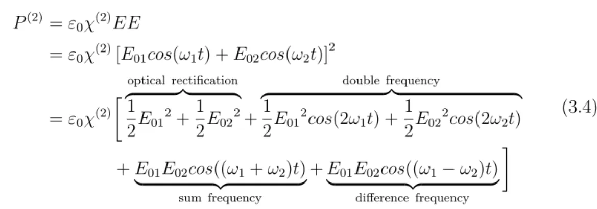
If two different wavelengths are used for the incoming beams, several differ- ent effects can occur additionally to the already mentioned ones. The incoming electric field can now be described by the sum of two planar waves.
E
=
E01cos (ω
1t) +E02cos (ω
2t)(3.3)
When plugging equation 3.3 into equation 3.2 one obtains, additionally to the
previous mentioned effects, the sum- and difference frequency of the two incoming
wavelengths.
3.1. Sum Frequency Generation Spectroscopy
P(2)
=
ε0χ(2)EE=
ε0χ(2)[E
01cos(ω1t) +E02cos(ω2t)]2=
ε0χ(2)optical rectification
z }| {
1
2
E012+ 1
2
E022+
double frequency
z }| {
1
2
E012cos(2ω1t) +1
2
E022cos(2ω2t)+
E01E02cos((ω1+
ω2)t)
| {z }
sum frequency
+
E01E02cos((ω1−ω2)t)
| {z }
difference frequency
(3.4)
In this equation all processes shown in the Jablonski diagram (figure 3.2) are covered. DFG (Difference Frequency Generation) is basically very similar to the optical rectification (P (0)), with the difference that two different incoming lasing frequencies are used. Therefore the resulting frequency is not zero but the difference of the two incoming frequencies.
ω
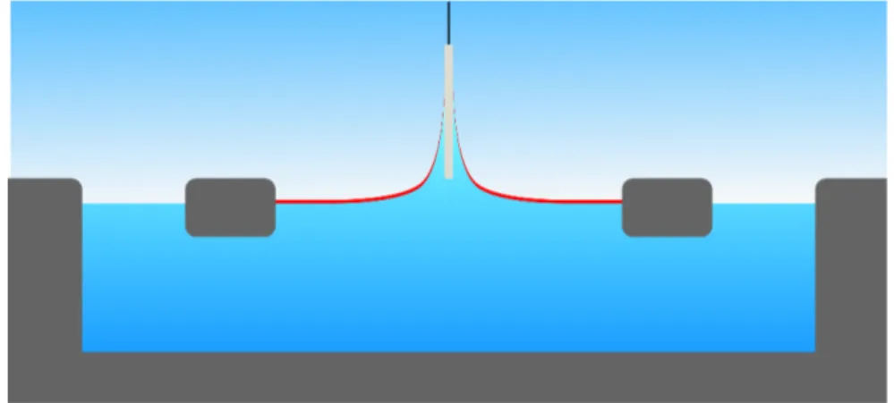
SFGFigure 3.3.: Schematic sketch of the SFG setup. Two laser beams, a visible one at 532 nm (ωvis) and a tunable in the infrared range (ωIR) hit the surface with temporal and spacial overlap. Among other contribution the sum frequency (ωSFG) is formed.
SFG is similar to SHG (see section 3.3.7), but with two incoming frequencies.
This is the spectroscopic method used for investigations in this work. Two laser beams, usually one tunable wavelength and one with a fixed wavelength hit the surface with spacial and temporal overlap. The temporal overlap is of course obsolete for continuous wave (cw) lasing systems, however, these systems are usually not used for this application. The great advantage of pulsed systems is the high energy used for spectroscopy, which can dissipate before the next pulse excites the system again. The schematic setup is shown in figure 3.3. A fixed visible beam and a tunable infrared beam hit the surface. Due to nonlinear effects, additionally to the incoming beams, higher order beams are generated, among them the sum frequency beam. With the assistance of notch filter and screens only the SFG-contribution reaches the detector.
3.1.2. Selection Rules of SFG
SFG is – as already mentioned – a surface specific technique. Only non-centro- symmetric matter gives rise to a second order nonlinear signal. No matter where this condition occurs a signal will be measured. An isotropic distributed liquid moving according to the Brownian motion has no preferential orientation. This is not a result from a certain setup, but an inherent feature of this technique. SFG is a two photon process. The intensity of the SFG-signal
ISFGis proportional to the intensities of the two incoming beams
Ivisand
IIRand to the square of the nonlinear susceptibility
χ(2).
ISFG ∝IvisIIR χ(2)2
(3.5) The nonlinear susceptibility is the link between the macroscopic observable in- tensity and the microscopic hyperpolarizability. It is material dependent and can be rewritten in terms of the oriental average of the hyperpolarizability
< βαβγ >.χ(2)
=
N < βαβγ >(3.6)
Nis the number density.
< βαβγ >is a microscopic quantity which is proportional to the IR- and Raman-transition dipole moments.
57βαβγ
= 1 2
~MαβAγ
(ω
vis−ωIR−iΓ)(3.7)
3.1. Sum Frequency Generation Spectroscopy
SFG ωvis
ωIR
ωSFG=ωvis+ωIR
|g>
|v>
|s>
Figure 3.4.: Jablonski diagram of a SFG-transition. Visible (green) and infrared (red) light hit the nonlinear medium and the sum frequency is generated (blue). The ground state is denoted as |g >, in the resonance case|v >is the excited state, other- wise both,|v >and |s >, are virtual states.
Mαβ
and
Aγare the corresponding Raman and IR transition dipole moments.
Mαβ
=
Xs
< g|µα|s >< s|µβ|v >
~
(ω
SFG−ω) −< g|µβ|s >< s|µα|v >~
(ω
vis−ω)
(3.8)
Aγ=< v
|µγ|g >(3.9) When plugging equations 3.6 and 3.7 into equation 3.5, it becomes clear that only transitions are allowed which are simultaneously IR- and Raman-active.
This can be only accomplished if the material is not centro-symmetric. This can
be rationalized by a thought experiment. Lets go back to equation 3.4. The
polarization of matter is proportional to the two incoming electric fields and the
second order susceptibility.
ε0is a constant. Solving the equation system reveals
that the only solution is no polarization at all and therefore no signal.
P~(2)∝χ(2)E ~~E
⇓i
−P~(2) ∝χ(2)
(
−E)(~ −E) =~ χ(2)E ~~E⇓
−P~(2)
= +
P~(2)⇓ χ(2)
= 0
(3.10)
This simple consideration is the reason why SFG is a surface specific technique.
When taking a look on the structure of a soft bulk matter, one realizes that the structure is overall centrosymmetric. The molecules are statistically distributed with no preferential orientation. Soft matter is - other than crystals - isotropic in all directions of space. This means that no second-order nonlinear process is possible. Only at the interface the isotropic distribution is broken. The ions have a preferential orientation and there is no more an inversion symmetric counter- part for each molecule. Therefore, in this region
χ(2)is not any more zero, and there is a SFG contribution. The depth of this contribution is not easily distin- guishable, because it strongly depends on the system. A surface covered with a charged lipid will have better and larger ranged net orientation than the pure air-water interface. This is the large difference of the surface specificity of non- linear optical techniques compared to other surface specific optical techniques.
The investigated depth is not dependent on the diffraction limit but only on the interfacial structure. This makes it possible to work with visible light with a ver- tical resolution in the range of a few molecule layers.
43It is very hard to estimate the exact depth resolution, especially since there is a fluent transition from the partially ordered surface to the isotropic bulk.
3.1.3. Signal Intensity
The SFG signal is given by the integral of the orientational distribution function
from one bulk phase over the interface to the adjacent bulk phase. This depends
on several factors. As discussed previously, molecules adopt a preferential ori-
entation at the interface, which is the basis for the SFG signal. The resulting
signal depends on three parameters: 1. The intensity of the signal, a high in-
tensity resonance gives a stronger signal. 2. The number of orientated molecules
3.1. Sum Frequency Generation Spectroscopy
is proportional to the intensity, because more molecules contribute to the signal.
3. The better the molecules are orientated, the higher the resulting signal will be. The first parameter is specific for the species, but when the same species is probed in different surroundings, then the intensity is only a function of the two latter parameters.
Figure 3.5.: Possible arrangement of molecules at the surface.