Contributions to Modeling Extreme Events on Financial and Electricity Markets

(1)

Financial and Electricity Markets

Inauguraldissertation zur

Erlangung des Doktorgrades der

Wirtschafts- und Sozialwissenschaftlichen Fakult¨ at der

Universit¨ at zu K¨ oln 2013

vorgelegt von

M.Sc. Volodymyr Korniichuk aus

Kuznetsovsk (Ukraine)

(2)

Korreferent: Prof. Dr. Karl Mosler

Tag der Promotion: 21.01.2014

(3)

Acknowledgements

I carried out the research underlying the material of this thesis at the University of Cologne under the supervision of Dr. Hans Manner and Dr. Oliver Grothe. I am sincerely grateful to my supervisors for their constant support in my professional and personal development, for their critical advice that has so often shown me the right direction, and for their patience during our countless discussions. This dissertation would have never been accomplished without a wise assistance of my supervisors. I would also like to thank Prof. Dr. Karl Mosler, who kindly agreed to be my external examiner.

The financial and research support through the Cologne Graduate School is gratefully acknowl- edged. CGS has been a constant source of encouragement where I have experienced an excellent academic environment and a very friendly atmosphere. Many thanks go to my colleagues from CGS and to Dr. Dagmar Weiler.

Finally, I would like to thank my parents Ludmila and Volodymyr Korniichuk, my brother Andriy, and Olena Pobochiienko for their unconditional support.

i

(4)

Acknowledgements i

List of Figures iv

List of Tables vii

Introduction 1

1 Modeling Multivariate Extreme Events Using Self-Exciting Point Processes 7

1.1 Motivation . . . 7

1.2 Model . . . 10

1.2.1 Univariate model . . . 11

1.2.1.1 Self-exciting POT model . . . 11

1.2.1.2 Decay and impact functions . . . 13

1.2.1.3 Stationarity condition and properties of the SE-POT model . . . 14

1.2.1.4 Relationship of SE-POT and EVT . . . 18

1.2.2 Multivariate Model . . . 19

1.2.2.1 Model Construction . . . 19

1.2.2.2 A closer look at the model implied dependence . . . 24

1.2.3 Properties of the multivariate model . . . 26

1.2.3.1 Joint conditional distribution of the marks . . . 26

1.2.3.2 Probabilities of exceedances in a remote region . . . 27

1.2.3.3 Contagion mechanism . . . 27

1.2.3.4 Risk Management implications . . . 29

1.3 Estimation, Goodness-of-Fit and Simulation . . . 31

1.3.1 Univariate model estimation . . . 31

1.3.2 Multivariate model estimation . . . 32

1.3.3 Goodness-of-fit . . . 33

1.3.4 Simulation . . . 34

1.4 Application to Financial Data . . . 35

1.4.1 Data and Preliminary Analysis . . . 36

1.4.2 Copula Choice . . . 36

1.4.3 Applying the Model . . . 37

1.4.3.1 Two-dimensional Model . . . 37

1.4.3.2 Four-dimensional Model . . . 41

1.5 Conclusion . . . 45

Appendices 47

A Method of Moments 48

B Extreme value condition and the initial threshold 50

ii

(5)

C Marginal goodness-of-fit tests 53 D Goodness-of-fit for the bivariate model with the MM estimates 55 E Goodness-of-fit for the sub-models of the four-dimensional model 57

2 Forecasting extreme electricity spot prices 59

2.1 Motivation . . . 59

2.2 Defining a price spike . . . 60

2.3 Modeling magnitudes of the spikes . . . 63

2.3.1 Description of the model . . . 63

2.3.1.1 Modeling long tails in magnitudes of the spikes . . . 63

2.3.1.2 Modeling dependence in magnitudes of the spikes . . . 65

2.3.1.3 Estimation . . . 68

2.3.1.4 Simulation and Goodness-of-fit . . . 68

2.3.2 Accounting for the price ceiling in magnitudes of the spikes . . . 69

2.3.3 Estimation results . . . 70

2.4 Modeling durations between spike occurrences . . . 73

2.4.1 Spike durations . . . 74

2.4.2 Models for the spike durations . . . 74

2.4.3 Negative binomial duration model . . . 75

2.4.3.1 Model description . . . 76

2.4.3.2 Estimation . . . 77

2.4.3.3 Simulation and Goodness-of-fit . . . 77

2.4.4 Estimation results . . . 78

2.5 Forecasting extreme electricity prices . . . 80

2.5.1 Forecasting approach . . . 80

2.5.2 Out-of-sample forecasting performance . . . 81

3 Estimating tails in top-coded data 85 3.1 Motivation . . . 85

3.2 Preliminaries . . . 86

3.2.1 Tail index . . . 86

3.2.2 Top-coding . . . 87

3.2.3 Regularly varying tails . . . 88

3.2.4 Distribution of Exceedances . . . 90

3.3 GPD-based estimator on top-coded data . . . 90

3.3.1 GPD and extreme value distributions . . . 91

3.3.2 Estimation of GPD on excesses under top-coding . . . 92

3.3.3 Properties of cGPD estimator: X ∼GP D . . . 94

3.3.4 Properties of cGPD estimator: X ∼EV D . . . 97

3.4 Hill estimator on top-coded data . . . 100

3.5 Comparison of cGPD and cHill . . . 103

3.6 Applications . . . 106

3.6.1 Simulation study . . . 106

3.6.2 Application to electricity prices . . . 110

Conclusion 114

Bibliography 116

(6)

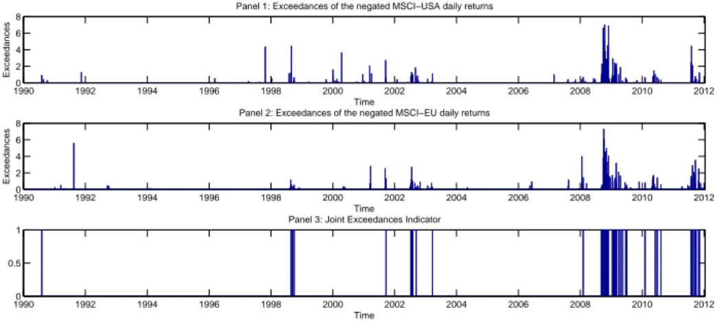
1.1 Exceedances of negated MSCI-USA (Panel 1) and MSCI-EU (Panel 2) daily log- returns over the respective 0.977th quantiles. Bar plot indicating times of the

joint exceedances (Panel 3). . . 8

1.2 Probability of a joint extreme event at time pointtconditioned on the event that at least one of the margins jumps att. . . 28

1.3 π₂(t, t⁺): instantaneous average number of second margin exceedances in the unit interval triggered by the increase of ∆_t,t+τ1(s, u1) (x-axis) in the first margin’s conditional rate. . . 28

1.4 π(t, t⁺): increase in the rate of the joint exceedances triggered by a joint exceedance at timet. . . 29

1.5 Estimated conditional rate of the marginal exceedances over the initial threshold for MSCI-USA and MSCI-EU. MLE estimates from Table 1.2. . . 39

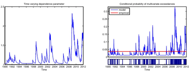
1.6 The estimated time-varying dependence parameter (left-hand panel) and the conditional probability of multivariate events when at least one margins exceed the initial threshold (right-hand panel) in the two dimensional model. The tick marks at the bottom of the right panel denote times of multivariate events. . . 40

1.7 Effects of different values of MSCI-EU and MSCI-US negated returns, that could have happened on 01.03.2009 (left panel) and 15.02.2010 (right panel), on the next day’s conditional rate of joint exceedances. . . 40

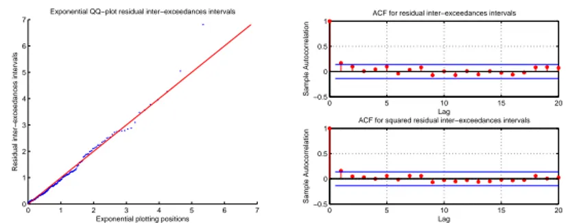
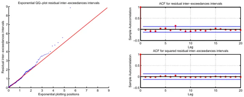
1.8 Exponential QQ-plot of the residual inter-exceedance intervals (left-hand panel) in the bivariate model. The sample autocorrelation function of those (squared) intervals (right-hand panel). . . 41

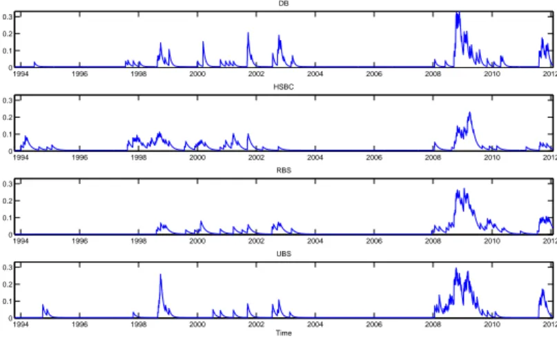
1.9 The estimated conditional rates of the marginal exceedances over the initial threshold in the SE-POT model for negated log-returns of DB, HSBC, RBS, and UBS stocks. . . 42

1.10 The estimated time-varying dependence parameter (left-hand panel) and the conditional probability of multivariate events when at least one margins exceed the initial threshold (right-hand panel) in the four-dimensional model. The tick marks at the bottom of the right panel denote times of multivariate events. . . 44

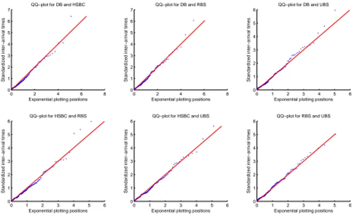
1.11 Exponential QQ-plot of the residual inter-exceedances intervals in the four-dimensional model (left-hand panel). The sample autocorrelation function of those (squared) intervals (right-hand panel). . . 44

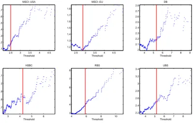
B.1 Sample mean excess plots of negated daily log-returns of the MSCI-USA, MSCI- EU, DB, HSBC, RBS, and UBS. Solid red vertical lines indicate the initial threshold chosen for the model estimation. . . 50

B.2 Estimated Q-curves on negated returns of MSCI-USA and MSCI-EU:kde- notes the number of upper order statistics used for estimation. . . 51

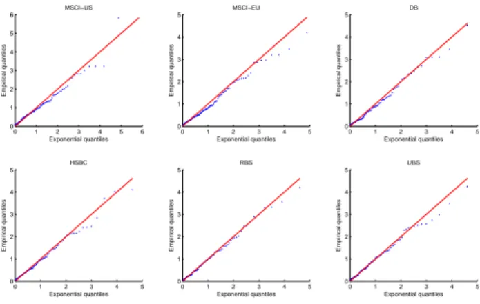
B.3 Exponential QQ-plots of time intervals, measured in days, between consecutive marginal exceeances above the initial threshold. . . 51

B.4 Estimated Q-curves on negated log-returns of DB, HSBC, RBS, and UBS. . . 52

C.1 Exponential QQ-plot of the residual marginal inter-exceedances intervals. . . 53

C.2 Exponential QQ-plot of the residual marks. . . 53 iv

(7)

D.1 Estimated conditional rate of the marginal exceedances over the initial threshold for MSCI-USA and MSCI-EU. MM estimates from Table 1.2. . . 55 D.2 The estimated time-varying dependence parameter (left-hand panel) and the con-

ditional probability of multivariate events when at least one margins exceed the initial threshold (right-hand panel) in the two dimensional model. The tick marks at the bottom of the right panel denote times of multivariate events. MM estimates. 55 D.3 Exponential QQ-plot of the residual inter-exceedance intervals (left-hand panel)

in the bivariate model. The sample autocorrelation function of those (squared) intervals (right-hand panel). MM estimates. . . 56 E.1 Exponential QQ-plot for the residual inter-exceedance intervals of the bivariate

sub-models of the four-dimensional model. . . 57 E.2 Exponential QQ-plot for the residual inter-exceedance intervals of the trivariate

sub-models of the four-dimensional model. . . 58 2.1 Electricity prices in NSW region of Australia’s electricity market over the period

Jan 1, 2002–Dec 31, 2011. . . 60 2.2 Mean and standard deviation of the electricity prices pooled by 30-min period of

the day. . . 61 2.3 Diurnal threshold. Note: solid vertical lines illustrate parts of the day where

parameterξof the GPD can be assumed to be the same, details in Section 2.3.1.1. 62 2.4 Monthly proportions of the spikes. Note: the period of atypically high proportion

of spikes in 2007 will be removed in modeling occurrences times of the spikes. . . 62 2.5 Sequential sample second moments of the electricity prices on the NSW region.

The second moments were calculated on the electricity prices from the 1st Jan 2002 to the time point denoted on x-axis. . . 63 2.6 Mean excess functions calculated for the NSW electricity prices pooled by 1st,

14th, 19th, 36th, 45th, and 48th half-hour period of the day. . . 64 2.7 Spearman’s rank correlation between the lagged spike magnitudes. . . 65 2.8 Histogram of the electricity prices exceeding 400AUD/MWh. . . 65 2.9 Autocorrelation of the residuals. Solid vertical lines show 99% confidence intervals. 72 2.10 QQ-plot of the transformed residuals. Green points show expected deviations of

the residuals. . . 72 2.11 QQ-plot of the standardized durations (transformed by the theoretically implied

distribution to the standard exponential) of the estimated ACD models and the residual inter-arrivals times of the estimated Hawkes process. The models were estimated on NSW spike durations occurred in the period over January 1, 2008–

December 31, 2010. . . 75 2.12 Density function of the negative binomial distribution. . . 76 2.13 QQ-plot of a typical sample of the estimated transformed generators. Compare

this figure with Figure 2.11. . . 79 2.14 The conditional probability of a spike occurrence on the four regions of Australia’s

electricity market. The probability was estimated according to (2.18) with parameters values from Table 2.6. p_i was set on its max achievable value: p_i = 0.0016 for NSW;p_i= 0.0017 for QLD;p_i = 0.0232 for SA;p_i= 0.0335 for VIC. . . 81 3.1 Influence function. . . 88 3.2 Mean (left panel) and standard deviation (right panel) of the asymptotic distri-

bution of the cGPD estimators. For this illustration the parameters are set as follows: ξ= 1/2,µ= 1/3,ρ=−1/5. . . 100 3.3 Mean (left panel) and standard deviation (right panel) of the asymptotic distribu-

tion of the cHill estimator. For this illustration the parameters are set as follows:

ξ= 1/2,µ= 1/3,ρ=−1/5. . . 103

(8)

3.4 R_{M SE}(ξ, ρ, λ_∗) for various sets of the parameters ξ, ρ, λ_∗. Note: instead of λ_∗ we report on the figureλ^−1/ξ_∗ , which shows what proportion of the exceedances is top-coded. . . 106 3.5 Estimates of ξ by the cGPD and the cHill estimators for the Parameter-set 1.

Panel 1 and 3 correspond to the cGPD estimates. Panel 2 and 4 correspond to the cHill estimates. . . 108 3.6 Estimates of ξ by the cGPD and the cHill estimators for the Parameter-set 2.

Panel 1 and 3 correspond to the cGPD estimates. Panel 2 and 4 correspond to the cHill estimates. . . 109 3.9 Daily maximum of SA electricity spot prices (since the data is very volatile, rang-

ing from 15AUD/MWh to 12500AUD/MWh, it is plotted on the log-scale) . . . 111 3.10 Sample mean excess plots of daily maximum of SA electricity spot prices. A solid

red vertical line indicates the thresholdu1,N chosen for the estimation ofξ. . . . 111 3.11 Excess distribution functions implied by the cGPD and the cHill estimators com-

pared to the empirical excess distribution function of the exceedances of daily maxima of SA electricity prices. . . 112

(9)

List of Tables

1.1 Summary statistics . . . 36 1.2 Parameter estimates of the SE-POT model by the MLE and the MM. An inverse

Hessian of the likelihood function is used to obtain the standard errors reported in parentheses right to the MLE estimates. . . 38 1.3 Parameter estimates of the dependence parameter. An inverse Hessian of the

likelihood function is used to obtain the standard errors reported in parentheses right to the MLE estimates. . . 39 1.4 MLE parameter estimates of the SE-POT model. An inverse Hessian of the likeli-

hood function is used to obtain the standard errors reported in parentheses right to the estimates. . . 41 1.5 p-values of the likelihood tests testing hypothesis that the bivariate dependence

structure in the four-dimensional model is symmetric. . . 42 1.6 Parameter estimates of the four-dimensional model of exceedances. An inverse

Hessian of the likelihood function is used to obtain the standard errors reported in parentheses right to the estimates. . . 43 1.7 p-values the Kolmogorov-Smirnov (KS) and Ljung-Box (LB) with 15 lags tests for

residual inter-exceedances intervals for the two- and three-dimensional sub-models of the four-dimensional model. . . 44 C.1 p-values of Kolmogorov-Smirnov (KS) and Ljung-Box (LB) tests checking the

hypothesis of exponentially distributed and uncorrelated residual inter-exceedance intervals and marks of the marginal processes of exceedances. . . 54 2.1 Descriptive statistics for half-hourly electricity spot prices (AUD/MWh) from the

four regions of Australia’s electricity market in the period over January 1, 2002–

December 31, 2011. . . 61 2.2 Parameter estimates of the model for spike magnitudes. . . 71 2.3 Estimated mean, standard deviation (std), mean relative bias (MRB), and mean

squared error (MSE) of estimated parameters for the ceiling adjusted model from 500 simulated paths. . . 72 2.4 Descriptive statistics of the actual and simulated prices (500 simulations). . . 73 2.5 Descriptive statistics for the spikes durations. . . 74 2.6 Parameter estimates of the negative binomial duration model estimated on the

spike durations. . . 78 2.7 Goodness-of-fit test: non-rejection rates (in %) of the Kolmogorov-Smirnov and

Ljung-Box (10 lags) tests with a significance level of 1% conducted on 1000 random samples of the estimated generators. . . 78 2.8 Descriptive statistics of the actual and simulated durations (500 simulations). . . 79 2.9 Out-of-sample performance of the models in forecasting electricity prices exceeding

300AUD/MWh. . . 82 2.10 Out-of-sample performance of our model in forecasting electricity prices exceeding

500AUD/MWh, 1000AUD/MWh, 2000AUD/MWh, and 5000AUD/MWh levels. 83 3.1 Estimated bias, standard deviation, and mean squared error (MSE) of estimates

ofξby the cGPD and cHill estimators (1000 simulations). . . 110 vii

(10)

Words like extremes, extremal events, worst case scenarios have long become an integral part in the vocabulary of financial researches and practitioners. This is not without reason. In view of the extreme and highly correlated financial turbulences in the last decades, the introduction of new (ill-understood) derivative products, and growing computerization of financial trading systems, it becomes evident that events that were believed to occur once in one hundred or even one thousand years (based on the standard financial models) tend to occur much more frequently than expected leading to severe unexpected losses on financial markets. Modeling and forecasting those extreme events is a topic of vivid interest and great importance in the current research of quantitative risk management and is exactly the topic of the thesis at hand.

In this thesis, we consider the problem of modeling very large (in absolute terms) returns on financial markets and focus on describing their distributional properties. Our aim is to design an approach that can accommodate the characteristic features of those returns, namely, heavy tails, contagion effects, tail dependence, and clustering in both magnitudes and times of occurrences. Additionally, the thesis contributes to the literature on forecasting extreme electricity spot prices. The challenge of this problem is determined, first, by the difficulty of modeling the price directories in high-frequency settings, and, second, by the distinctive feature of electricity, namely, its limited storability. Furthermore, in this thesis, we investigate a problem of estimating probability distributions whose tails decrease very slowly (heavy-tailed distributions). In particular, we study the properties of two popular estimators of those distributions in the case when the underlying data is top-coded, i.e., unknown above a certain threshold.

To cope with the task of describing extreme events, both an accurate quantitative analysis – a focus of this thesis – as well as a sound qualitative judgement are required. Considering the latter, for example, it is astonishing to see how many early warnings of the subprime crisis 2007 both in the press (see Danielsson [2013]) and in the academics (see Das, Embrechts, and Fasen [2013] and Chavez-Demoulin and Embrechts [2011] for an overview) were ignored by the regulators and practitioners. Examples of blunders with the quantitative analysis include, among others, an extensive reliance on correlation based risk measures, which are known to be often misleading, see Embrechts, McNeil, and Straumann [2002], and an often unjustified use of the Gaussian copula in the standard pricing formulas for tranches of collateralized debt obligations.

It is known from Sibuya [1959] that this copula underestimates the probability of joint extremal events, because it does not exhibit tail dependence, see Chavez-Demoulin and Embrechts [2011].

Whatever the reason of that misuse of quantitative methods in practice, the statistical modeling

1

(11)

of extreme events, as a crucial component in understanding heavy-tailed phenomena, needs to be further developed from a scientific point of view.

Currently there is general agreement that daily financial data is well described by (multivariate) distributions whose tails are much heavier than the ones of the normal distribution and whose dependence structure can accommodate clustering of extremes. Popular models that can partly fulfil the above requirements are generalized autoregressive conditional heteroskedastic- ity (GARCH) [Bollerslev, 1986] and stochastic volatility, see Shephard [1996] for an overview.

The popularity of those models is founded by their computational simplicity and ability to capture volatility clustering and heavy-tailed phenomena. Furthermore, a GARCH process can also account for clustering of extremes [Davis and Mikosch, 2009a]. In particular, large values of a GARCH process always occur in clusters, as opposed to a stochastic volatility process, whose large values behave similarly to extremes of the corresponding serially independent process [Davis and Mikosch, 2009b]. These findings imply that a GARCH model performs better than a stochastic volatility model in describing the timing of extreme events in financial data.

Although displaying very useful features, there are limitations for using GARCH processes. In particular, those processes do not seem to accurately capture the size of extremes in financial time series [Mikosch and St˘aric˘a, 2000]. Furthermore, the stationarity condition of GARCH processes restricts their applications to situations with finite variance. As it will be highlighted in Section 2 of the thesis, the assumptions of finite variance is inappropriate for modeling electricity spot prices. From a statistical point of view, extreme observations may also have strong deleterious effects on the parameter estimates and tests of a GARCH model [van Dijk, Franses, and Lucas, 1999].

Overall, extreme observations have its own unique features which differ substantially from the rest of the sample and hence cannot always be accommodated by models that are intended to describe the whole structure of the data. To capture those unique features, there is increased interest in approaches that use mainly extreme observations for inferences. This requirement calls for applications of extreme value theory. In this thesis, we will introduce models developed in the framework of that theory and consider specific problems of modeling extreme events on financial as well as electricity markets that have attracted much attention in the literature in recent years.

Extreme Value Theory (EVT) studies phenomena related to very high or very low values in sequences of random variables and in stochastic processes. EVT provides fundamental theoretical results and a multitude of probabilistic approaches to modeling heavy tails and extreme multivariate dependences. A basic result of the univariate EVT is the Fisher-Tippet-Gnedenko theorem, see de Haan and Ferreira [2006] (Theorem 1.1.3), which allows for modeling the maxima of a set of contiguous blocks of stationary data using the generalized extreme value distribution (up to changes of location and scale)Hξ(x) = exp

−(1 +ξx)^−1/ξ₊

. In particular, if for independent random variablesX₁, X₂, . . . with the same probability distribution function F, there exist sequencesan>0,bn∈R, such that

n→∞lim P

max (X1, X2, . . . , Xn)−bn

a_n ≤x

= lim

n→∞Fⁿ(anx+bn)→H(x)

(12)

where H(x) is a non-generate distribution function, then the only possible non-generate distribution H(x) is of the form Hξ(ax+b). Another model for extremes is provided by the Pickands-Balkema-de Haan theorem (see Pickands [1975], Balkema and de Haan [1974]), which is inherently connected to the previous model through a common basis of Karamata’s theory of regular variation. According to that theorem the distribution of excesses of a heavy-tailed random variable over a sufficiently high threshold is necessarily the generalized Pareto distribution (GPD) G(x;ξ, β) = 1−(1 +ξx/β)^−1/ξ₊ . The choice of that high threshold is however complicated in practice as it depends on the second order properties of the distribution function, see Chavez-Demoulin and Embrechts [2011]. Along with the GPD choice for the magnitudes of the excesses, the occurrence of those excesses follows a Poisson process, see Leadbetter [1991].

The results of the univariate EVT allow for the statistical modeling of common risk measures like Value-at-Risk (used more in banking) and expected shortfall (used more in insurance). Note however that application of the GPD and the generalized extreme value distribution is often confronted with a problem of interpretation of the parameters from a practitioner’s point of view (in contrast to mean and standard deviation of the normal distribution). A fundamental work considering the univariate EVT and applications of those models to financial data is Embrechts, Kl¨uppelberg, and Mikosch [1997], see also McNeil and Frey [2000] for estimation of tail related risk measures. Extensions of the univariate EVT to stationary time series which show a certain short-range dependence can be found in Leadbetter, Lindgren, and Rootzen [1983].

Multivariate extensions of the (classical) univariate EVT play also an important role in describing extreme events, especially considering their dependence structure. The basic result of the multivariate EVT concerns the limit multivariate distribution of the componentwise block maxima. In particular, if for independent and identically distributed random vectors (X1,i, . . . , Xd,i), i= 1,2, . . . there exist sequences a_k,n>0,b_k,n∈R,k= 1, . . . , dsuch that

n→∞lim P

max (Xk,1, , . . . , Xk,n)−bk,n

a_k,n ≤xk, k= 1, . . . , d

→H(x1, ..., xd)

whereH(x1, ..., xd) is a distribution function with non-degenerate marginals, thenH(x1, ..., xd) is a multivariate extreme value distribution. This distribution is characterized by the margins, which have the generalized extreme value distributions H_ξ_k(x) = exp

−(1 +ξ_kx)^−1/ξ₊ ^k , k = 1, . . . , d, and by copula C, referred to as extreme value copula, for which it holds

∀a >0,∀(u1, . . . , u_d)∈[0,1]^d:C(u₁, ..., u_d) =C^1/a(u^a₁, ..., u^a_d).

A specific dependence structure (not unique) implied by the above property provides useful copulas, for example Gumbel and Galambos copulas, for capturing the joint tail behavior of risk factors that show tail dependence. Applications and discussions of multivariate extreme value distributions can be found in de Haan and de Ronde [1998], Embrechts, de Haan, and Huang [2000], Tawn [1990], Haug, Kl¨uppelberg, and Peng [2011] and Mikosch [2005]. An extensive textbook treatment of EVT can be found in de Haan and Ferreira [2006] and Resnick [2007].

The solid theoretical background behind EVT makes its application for modeling extreme events natural and consequent. As it is noted in Chavez-Demoulin and Embrechts [2010], a careful use of EVT models is preferred above the casual guessing of some parametric models that may fit

(13)

currently available data over a restricted range, where only a few (if any) extreme observations are available. Due to the strict underlying assumptions and the non-dynamic character, however, the methods of EVT are not always directly applicable in situations where the extremes are serially dependent, as it is the case in almost all financial time series. This problem was discussed, among others, in Leadbetter, Lindgren, and Rootzen [1983], Chavez-Demoulin, Davison, and McNeil [2005], Chavez-Demoulin and McGill [2012], Davison and Smith [1990], Coles [2001] (Chapter 5), and see also Chavez-Demoulin and Davison [2012] for an overview.

In this thesis we will attempt to contribute to the literature by proposing models which extend the current results of EVT and offer new insight with modeling extreme events in serially dependent time series. In particular, we will review theoretical and practical questions that arise in the process of modeling extreme events on financial and electricity markets in daily and high- frequency settings. Under extreme events we understand situations when a financial parameter (e.g., equity return, electricity spot price) exceeds a characteristic high threshold (e.g., 99.9%th quantile). The questions of conditional modeling occurrence times and magnitudes (heavy tails) of those events as well as their complex dependence structure will be addressed.

Outline and summary

Chapter 1 deals with the problem of modeling multivariate extreme events observed in financial time series. The major challenge coping with that problem is to provide insights into the temporal- and cross-dependence structure of those extreme events in view of their clustering, which is observed both in their sizes and occurrence times, and specific dependence structure in the tails of multivariate distributions. Furthermore, those events demonstrate a certain synchronization in occurrences across markets and assets (e.g., contagion effects), which motivates the application of multivariate methods. To capture those characteristic features, we develop a multivariate approach based on self-exciting point processes and EVT. We show that the conditional rate of the point process of multivariate extreme events (constructed as a superposition of the univariate processes) is functionally related to the multivariate extreme value distribution that governs the magnitudes of the observations. This extreme value distribution combines the univariate rates of the point processes of extreme events into the multivariate one. Extensive references to the point process approach to EVT can be found in Resnick [1987]. Due to its point process representation, the model of Chapter 1 provides an integrated approach to describing two inherently connected characteristics: occurrence times and sizes of multivariate extreme events.

A separate contribution of this chapter is a derivation of the stationarity conditions for the self- exciting peaks-over-threshold model with predictable marks (this model was first presented in McNeil, Frey, and Embrechts [2005], Section 7.4.4). We discuss the properties of the model, treat its estimation (maximum likelihood and method of moments), deal with testing goodness-of-fit, and develop a simulation algorithm. We also consider an application of that model to return data of two stock markets (MSCI-EU, MSCI-USA) and four major European banks (Deutsche Bank, HSBC, UBS, and RBS).

Along with financial time series, electricity spot prices are also strongly exposed to sudden extreme jumps. Contrary to financial markets, where the reasons of turmoil are often explained by behavioral aspects of the market participants, in electricity markets the occurrence of extreme prices is attributed to an inelastic demand for electricity and very high marginal production

(14)

costs in the case of unforeseen supply shortfalls or rises in the demand for electricity. Due to the lack of practical ways to store electricity, those inelasticities and high marginal costs may manifest themselves in electricity prices that exceed the average level a hundred times. This type of price behavior presents an important topic for risk management research and is of great relevance for electricity market participants, for example, retailers, who buy electricity at spot prices but redistribute it at fixed prices to consumers. In Chapter 2 of this thesis we present a model for forecasting the occurrence of extreme electricity spot prices. The unique feature of this model is its ability to forecast electricity price exceedances over very high thresholds (e.g.

99.99%th quantile), where only a few (if any) observations are available. The model can also be applied for simulating times of occurrence and magnitudes of the extreme prices. We employ a copula with a changing dependence parameter for capturing serial dependence in the extreme prices and the censored GPD (to account for possible price ceilings on the market) for modeling their marginal distributions. For modeling times of the extreme price occurrences we propose a duration model based on a negative binomial distribution, which can reproduce large variation, a strong clustering pattern and the discrete nature of the time intervals between the occurrences of extreme prices. This duration model outperforms the common approaches to duration modeling:

the autoregressive duration models (Engle and Russell [1998]) and the Hawkes processes (Hawkes [1971]), see Bauwens and Hautsch [2009] for an overview. Once being estimated, our forecasting model can be applied (without re-estimation) for forecasting occurrences of price exceedances over any sufficiently high threshold. This unique feature is provided by a special construction of the model in which price exceedances over very high thresholds may be triggered by the price exceedances over a comparatively smaller threshold. Our forecasting model is applied to electricity spot prices from Australia’s national electricity market.

Another research question addressed in this thesis is the estimation of heavy-tailed distributions on top-coded observations, i.e., observations, whose values are unknown above a certain threshold. Not knowing the exact values of the upper-order statistics in the data, the top-coding (right-censoring) may have a strong effect on estimation of the main characteristic of the heavy- tailed distributions – the tail index, the decay rate of the power function that describes the distribution’s tail. This problem occurs, for example, in the insurance industry where, due to the policy limits on insurance products, the amount by how much the insurance claims (typically heavy-tailed) exceed those limits is not available. The tail index plays a crucial role in determining common risk measures (e.g., Value-at-Risk, expected shortfall) and is therefore required to be estimated accurately. In Chapter 3 we examine how two popular estimators of the tail index can be extended to the settings of top-coding. We consider the maximum likelihood estimator of the generalized Pareto distribution and the Hill estimator. Working in the framework of Smith [1987], we establish the asymptotic properties of those estimators and show their relationship to various levels of top-coding. For high levels of top-coding and small values of the tail index, our findings suggest a superior performance of the Hill estimator over the GPD approach. This result contradicts the broad conclusion about the performance of those estimators in the uncensored case as it was established in Smith [1987].

The main chapters of the thesis are based on academic papers. Chapter 1 is in line with Grothe, Korniichuk, and Manner [2012], which is a joint work of Oliver Grothe, Volodymyr Korniichuk, and Hans Manner, all of whom have contributed substantially to the paper. Korniichuk [2012]

(15)

underlies Chapter 2. Finally, Chapter 3 is based on Korniichuk [2013]. Since the papers underlying the chapters of the thesis are independent of each other, those chapters can be read in any order. Each of the chapters has a detailed introduction (motivation) and a conclusion. The final chapter of the thesis shortly summarizes the major contributions.

(16)

Modeling Multivariate Extreme Events Using Self-Exciting Point Processes

1.1 Motivation

A characteristic feature of financial time series is their disposition towards sudden extreme jumps.

As an empirical illustration consider Figure 1.1, which shows occurrence times and magnitudes of exceedances of MSCI-USA and MSCI-EU indices’ negated returns over a high quantile of their distributions. It is apparent from the figure that both occurrence times and magnitudes of the exceedances resemble a certain clustering behavior, namely, large negative returns tend to be followed by large ones and vice versa. Additionally, this clustering behavior is observed not only in time but also across the markets, which is manifested, among others, in the occurrence of joint exceedances. This synchronization of large returns’ occurrences may be attributed to the information transmission across financial markets, see, for example, Wongswan [2006], where, based on high-frequency data, international transmission of economic fundamental announcements is studied on the example of the US, Japan, Korean and Thai equity markets. Other channels of the informational transmission are described in Bekaert, Ehrmann, Fratzscher, and Mehl [2012], where, in particular, the authors provide a strong support for the validity of the “wake-up call”

hypothesis, which states that a local crisis in one market may prompt investors to reexamine their views on the vulnerability of other market segments, which in turn may cause spreading of the local shock to other markets. Clustering of extreme events may also be caused by intra-day volatility spillovers both within one market and across different markets, see Golosnoy, Gribisch, and Liesenfeld [2012] for a recent study of this topic. In general, it is not clear whether the joint exceedances are triggered by a jump in one component or just caused by a common factor – both scenarios occur in financial markets and are interesting to analyze. The behavior of extreme asset-returns presents an important topic for research on risk management and is of great relevance especially in view of the latest financial crisis.

7

(17)

19900 1992 1994 1996 1998 2000 2002 2004 2006 2008 2010 2012 2

4 6 8

Panel 1: Exceedances of the negated MSCI−USA daily returns

Time

Exceedances

19900 1992 1994 1996 1998 2000 2002 2004 2006 2008 2010 2012

2 4 6 8

Panel 2: Exceedances of the negated MSCI−EU daily returns

Time

Exceedances

19900 1992 1994 1996 1998 2000 2002 2004 2006 2008 2010 2012

0.5 1

Panel 3: Joint Exceedances Indicator

Time

Figure 1.1: Exceedances of negated MSCI-USA (Panel 1) and MSCI-EU (Panel 2) daily log- returns over the respective 0.977th quantiles. Bar plot indicating times of the joint exceedances

(Panel 3).

The problem of modeling jumps or exceedances above high thresholds in asset-returns was considered in many papers. For example, Bollerslev, Todorov, and Li [2013] approach this problem by partitioning jumps into idiosyncratic and systemic components, and by further direct modeling of the jumps’ distributional properties based on the results of extreme value theory. A¨ıt-Sahalia, Cacho-Diaz, and Laeven [2011] propose a Hawkes jump-diffusion model in which self-exciting processes (with mutual excitement) are used for modeling clustering of extreme events both in time and across assets. That paper develops a feasible estimation approach based on the generalized method of moments and provides strong evidence of self-excitation and asymmetric cross-excitation in financial markets. Modeling multivariate exceedances above high thresholds is also a topic of intensive research in extreme value theory. For example, it was shown in the literature that the multivariate generalized Pareto distribution is the natural distribution for multivariate extreme exceedances, see Smith, Tawn, and Coles [1997] and Rootzen and Tajvidi [2006]. Recent studies considering the estimation of the probability that a random vector falls in some remote region are Einmahl, de Haan, and Krajina [2013] and Drees and de Haan [2012].

Note, however, that those methods are not directly applicable when the extremes are clustering in time. Extensive treatments of EVT methods can be found in de Haan and Ferreira [2006] or Resnick [2007]. Studies that are related to modeling clusters in financial data are Bowsher [2007]

who introduces a new class of generalized Hawkes process (including non-linear models) and studies with its bivariate version the transaction times and mid-quote changes at high-frequency data for a NYSE stock, as well as Errais, Giesecke, and Goldberg [2010] who employ self-exciting processes for modeling portfolio credit risk, in particular, for the valuation of credit derivatives.

Considering the recent developments in modeling extreme asset-returns, there is still a demand for a model that can provide insights into the temporal- and cross-dependence structure of multivariate extreme events in view of their clustering and specific dependence structure in the tails of (multivariate) distributions. In this chapter of the thesis we develop a model that can fill this gap. Working in the framework of marked self-exciting point processes and extreme value theory (EVT), we model multivariate extreme events as a univariate point process being constructed as a superposition of marginal extreme events. For modeling the marginal processes

(18)

of exceedances we revise the existing specification of the univariate self-exciting peaks-over- threshold model of Chavez-Demoulin, Embrechts, and Neˇslehov´a [2006] and McNeil, Frey, and Embrechts [2005], which is able to cope with the clustering of extremes (in both times and magnitudes) in the univariate case. After this revision, we are able to formulate stationarity conditions, not discussed in the literature before, and to analyze the distributional properties of the model. This constitutes a separate contribution of this chapter of the thesis.

We show that the only way how the marginal rates can be coupled into the multivariate rate of the superposed process is through the exponent measure of an extreme value copula. The copula used for the construction of the multivariate rate follows naturally from EVT arguments, and is the same extreme value copula that governs the (conditional) multivariate distribution of the marginal exceedances at the same point of time. This result provides an integrated approach to modeling occurrence times and sizes of multivariate extreme events, because those two characteristics are inherently connected. Furthermore, the results provide insight into the dependence between point processes that are jointly subject to EVT. This is in contrast to alternative approaches in the literature, where the dependence between marginal point processes is incorporated through an affine mutual excitement, see, for example, A¨ıt-Sahalia, Cacho-Diaz, and Laeven [2011], Embrechts, Liniger, and Lin [2011], and magnitudes of the jumps (if considered) are modelled in a separate way.

Concerning the advantages of our method, it is worth noting that we use the data explicitly only above a high threshold. This allows us to leave the time series model for the non-extreme parts of the data unspecified. We consider the dependence structure of multivariate exceedances only in regions where the results from multivariate extreme value theory (MEVT) are valid. Further- more, the MEVT enables us to extrapolate exceedance probabilities far into remote regions of the tail where hardly any data is available. With such a model we are able to extract the probabilities of arbitrary combinations of the dimensions in any sufficiently remote region. Since the model captures clustering behavior in (multivariate) exceedances, and accounts for the fact that not only times but also sizes of exceedances may trigger subsequent extreme events, the model provides asymmetric influences of marginal exceedances so that spill-over and contagion effects in financial market may be analyzed. This model may be of great interest for risk management purposes. For example, we can estimate the probabilities that from a portfolio of, say,dassets, a certain subset falls in a remote (extreme) set conditioned on the event that some other assets (or at least one of them) from that portfolio take extreme values at the same point of time. We shortly discuss other possible risk management applications of the model and provide real data examples.

To estimate our proposed model, we derive the closed form likelihood function and describe the goodness-of-fit and simulation procedures. As noted earlier, our model treats a multivariate extreme exceedance as a realization of a univariate point process. This property is advantageous for the estimation, because, as it is mentioned in Bowsher [2007], there are currently no results concerning the properties of the maximum likelihood estimation (MLE) for multivariate point processes. For the univariate case, on the other hand, it is shown in Ogata [1978], that under some regularity conditions, the MLE for a stationary, simple point process is consistent and asymptotically normal. Inspired by A¨ıt-Sahalia, Cacho-Diaz, and Laeven [2011], we consider

(19)

also the model estimation based on method of moments, which, however, seems to underperform the MLE in the case of our model. The reason for this may lie in both the choice of moment conditions and in the fact that all moment conditions are based on the goodness-of-fit statistics, which cannot be directly calculated from the sample independently from the unknown parameters of the models.

In the empirical part of the chapter, we apply our model to study extreme negative returns on the financial markets (USA, Europe) and in the European banking sector (Deutsche Bank, RBS, HSBC, and UBS). The results of goodness-of-fit tests demonstrate a reasonable fit of the model and suggest an empirical importance of the self-exciting feature for modeling both occurrence times, magnitudes, and interdependencies of the extreme returns. We find that conditional multivariate distributions of the returns are close to symmetric with the strength of dependence strongly responding to individual jumps. Despite the symmetrical structure of the distribution, there are still asymmetric effects coming from the self-exciting structure of the conditional marginal distributions of the exceedances’ magnitudes. This self-exciting structure provides also a natural way how to model time-varying volatility of the magnitudes and, hence, their heavy tails.

The rest of the chapter is structured as follows. The model and its properties are derived in Section 1.2. In Section 1.3 we describe estimation of the model, along with the goodness-of-fit and simulation procedures. Section 1.4 presents applications of the model to financial data and Section 1.5 concludes. Finally, some of the goodness-of-fit graphs and intermediary calculations are relegated to the Appendix.

1.2 Model

The major challenges in constructing the model presented in this section are twofold. First, the model should capture the distinctive features of multivariate extreme events typically observed in financial markets, namely, clustering and spillover effects. Second, the model should be able to account for the specific distributional properties of magnitudes of extreme observations (i.e., for the distributions over the threshold). For both reasons, our model is developed in the framework of extreme value theory and marked point processes.

Throughout the text we use the following notation. Consider a random vectorX_t= (X_1,t, . . . , X_d,t) which may, e.g., represent daily (negated) log-returns ofdequities at timet. Byu= (u1, . . . , ud), theinitial threshold, we denote a vector with components relating to sufficiently high quantiles of the marginal distributions of X_t. We focus on the occurrence times as well as the magnitudes of multivariate extreme observations, which we define as situations when Xt exceeds u in at least one component. Under ani-th marginal extreme event we understand the situation when X_i,t > u_i. We refer to such extreme events as marginal exceedances and characterise them by occurrence timesTi,1, Ti,2, . . .and magnitudes (themarks) of realizations ˜Xi,1,X˜i,2, . . ., i.e., ˜Xi,k=Xi,T_i,k. The history that includes both the times and magnitudes of exceedances of (Xi,s)_s<taboveuiwill be denoted asH^i,tand the combined history over all marginal exceedances is denoted asHt=Sd

i=1Hi,t.

(20)

This section is structured as follows. Section 1.2.1 deals with the univariate self-exciting peaks- over-threshold model, which is the basis for our multivariate model developed in Section 1.2.2.

Section 1.2.3 provides some properties of the multivariate model.

1.2.1 Univariate model

This section deals with the univariate self-exciting peaks-over-threshold model. After a short review of this model, we reconsider some parts of its construction to enrich it with some new useful properties. In particular, we suggest a new specification for the impact function which, contrary to its existing specification, provides an intuitively reasonable mechanism how past exceedances trigger the future ones (Section 1.2.1.2), allows us to set a stationarity condition and to develop some distributional properties of the univariate model (Section 1.2.1.3). Finally, in Section 1.2.1.4 we consider the relationship of the univariate self-exciting peaks-over-threshold model to the general framework of the extreme value theory.

1.2.1.1 Self-exciting POT model

The basic setup to model univariate exceedances is to assume independent and identically distributed (iid) data and to use a peaks-over-threshold (POT) model developed in Davison and Smith [1990] and Leadbetter [1991]. In the framework of EVT, the POT model is based on the asymptotic behavior of the threshold exceedances for iid or stationary data if these are in the maximum domain of attraction of some extreme value distribution. If the threshold is high enough, then the exceedances occur in time according to a homogeneous Poisson process and the mark sizes are independently and identically distributed according to the generalized Pareto distribution (GPD).

The self-exciting POT model presented in Chavez-Demoulin, Davison, and McNeil [2005] ex- tends the standard set-up of the POT model by allowing for temporal dependence between extreme events. This temporal dependence is introduced into the model by modeling the rate of occurrences in the standard POT method with self-exciting processes, see Hawkes [1971].

Definition 1.1. (Self-exciting point process) A point processN(t), representing the cumulative number of events up to timet, is called a (linear) self-exciting process with the conditional rate τ(t), if

P (N(t+ ∆)−N(t) = 1|Ht) =τ(t)∆ +o(∆), P (N(t+ ∆)−N(t)>1|Ht) =o(∆) with

τ(t) =τ+ψ Z t

−∞

c X˜s

g(t−s)dN(s), τ >0, ψ≥0,

where ˜Xsindicates the event’s mark at times. The impact functionc(·) determines the contribution of events to the conditional rate and the decay functiong(·) determines the rate how an influence of events decays in time. When no mark is associated with the eventc

X˜_s

≡1.

(21)

Choices of impact and decay functions are discussed in Section 1.2.1.2. The self-exciting POT is further extended in McNeil, Frey, and Embrechts 2005, where the temporal dependence is incorporated also into the conditional distribution of the marks, i.e., also the distribution of the marks depends on past information. We refer to this model as theself-exciting POT model with predictable marks (SE-POT). For convenience and consistency of notation we present the model using subindizesi = 1. . . d which will later refer to the dimensions of our multivariate model.

In the SE-POT model, the rate of crossing the initial thresholdui is modelled by a self exciting point process where the rate is parametrized as

τ_i(t, u_i) =τ_i+ψ_iv^∗_i(t), τ_i>0, ψ_i≥0, (1.1) with

v_i^∗(t) = Z t

−∞

c_i(X_i,s)g_i(t−s)dN_i(s), (1.2) where againc_i(·) andg_i(·) denote, respectively, the impact and decay functions, andN_i(s) is a counting measure ofi-th margin exceedances.

Additionally, the excesses over the thresholdui are now assumed to follow the GPD with shape parameterξ_i and time varying scale parameterβ_i+α_iv^∗(t). In particular, forx_i > u_i,

P (Xi,t≤xi|Xi,t > ui,Hi,t) = 1−

1 +ξi

xi−ui

βi+αiv_i^∗(t) −1/ξi

=:Fi,t(xi), βi>0, αi≥0.

(1.3) This distribution covers the cases of Weibull (ξ_i<0), Gumbel (ξ_i= 0) and Fr´echet (ξ_i>0) tails, corresponding to distributions with finite endpoints, light tails, and heavy tails, respectively. For ξi= 0, the distribution function in (1.3) should be interpreted as Fi,t(xi) = 1−e^−xⁱ. Finally, due to the GPD as the conditional distribution of the marks, the conditional rate of exceeding a higher thresholdx_i ≥u_i scales in the following way

τi(t, xi) =τi(t, ui)

1 +ξi

xi−ui

β_i+α_iv^∗_i(t) −1/ξi

, xi≥ui, (1.4)

where τi(t, ui) is the rate of crossing the initial threshold ui given by Equation (1.1). The conditional rateτi(t, xi) explicitly describes the conditional distribution of times of exceedances above any thresholdx_i≥u_i in the following way.

P T_i,k+1(x_i)≤t|Hi,T_i,k(x_i)

= 1−exp − Z t

T_i,k(x_i)

τ_i(s, x_i)ds

!

, t≥T_i,k(x_i), (1.5)

whereTi,k(xi) denotes (random) time of thek-th exceedance of (Xi,s)_s∈Rabovexi. The above relationship is a direct consequence of the definition of the conditional intensity as the combina- tion of hazard rates of the time intervals between exceedances, see Daley and Vere-Jones [2005], p. 231. There is a small abuse of notation in the equation above, as, to make the notation easy, we interchange the use of a hazard rate, a deterministic function, with the conditional intensity, a piecewise determined amalgam of hazard rates.

Note that the self-exciting componentv_i^∗(t) enters bothτi(t, ui) in (1.1) andFi,tin (1.3) and thus provides a specific “clustering mechanism” into the conditional distribution of both times and

(22)

marks of exceedances. After an exceedance occurs at time t₀ with mark x₀, the function v_i^∗(·) jumps byci(x0) and increases the instantaneous probability of the exceedance’s occurrence and the marks’ volatility (through time-varying scale parameter βi(t)). In absence of exceedances v_i^∗(·) tends towards zero through function g_i(·). Being a transmitter of information of past exceedances to the future ones, the function v_i^∗(·) may be interpreted as a kind of volatility measure of extreme exceedances. This interpretation may be found also in Bowsher [2007], where the estimated mid-quote intensity is used as approximation to the stock price’s instantaneous volatility.

The clustering mechanism of the SE-POT model, how past exceedances may trigger the occurrence of future exceedances, can quite accurately describe the cluster behavior of extreme exceedances observed on financial markets, see Chavez-Demoulin and McGill [2012]. That is why the SE-POT model is chosen as a cornerstone for our multivariate model developed in Section 1.2.2.

Because of the overall importance of the SE-POT model for our multivariate model, in the next sections we develop some of its distributional properties, including a stationarity condition, and reconsider the existing specifications for the decay and impact functions.

1.2.1.2 Decay and impact functions

Considering functional specification of the decay and impact functions in (1.2) there are advantages in some specific forms. The decay function chosen in this thesis is g(s) = e^−γs, γ > 0 (the subindex “i” is dropped), which is a popular specification suggested in Hawkes [1971]. This specification makes the self-exciting process a Markov process [Oakes, 1975] and leads to a simple formula for the covariance density (derived in Proposition 1.3). This choice is also motivated in view of Boltzman’s theory of elastic after-effects, see Ogata [1988], p.11. An alternative is the functiong(s) = (s+γ)^−(1+ρ), withγ, ρ >0. This specification originally comes from seismology, where is known as Omori law, see Helmstetter and Sornette [2002]. Due to the substantial advantages in deriving the analytical formulas, we will stick tog(s) =e^−γsthroughout this chapter of the thesis.

The aim of the impact functionc(·) is to capture the effect of the marks of exceedances onto the conditional rate of future exceedances. A popular choice isc(x) =e^δx,see for example Chavez- Demoulin and McGill [2012] or McNeil, Frey, and Embrechts [2005] (Section 7.4.3). However, an important point to consider when specifying that function is to ensure its ability to accurately extract information from the marks. Provided the conditional distribution of the marks is time- varying (as it is indeed the case with the SE-POT model, see (1.3)), one expectsc(·) to account not only for the magnitudes of the marks but also for the conditional distribution from which they were drawn. To put it differently, not the size of the mark but its quantile in the corresponding conditional distribution is decisive in determining the effect of the mark onto the conditional rate. Thus, instead of specifyingc(·) as a fixed function, we suggest the following specification

c(x_t) =c^∗(F_t(x_t)),

(23)

whereF_tis the marks’ conditional distribution (1.3) andc^∗(·) is an increasing function [0,1]→ [1,∞]. This specification can properly capture the time-varying impact of an exceedance on the conditional rate. An easy way to construct c^∗(·) is as c^∗(·) = 1 +G^←(·), where G^←(·) is the inverse of a distribution functionGof some continuous positive random variable with finite mean δ. With suchc^∗(·) the impact function takes the form

c(x_t) = 1 +G^←(F_t(x_t)). (1.6)

We will use the above specification for the impact function throughout the text. In the empirical part of this chapter, we will use G^← of an exponential distribution, which yields c^∗(u) = 1− δlog(1−u).

Besides the appropriate extraction of information from the marks, the choice (1.6) for the impact function is advantageous overc(x) =e^δx, because (1.6) allows us to set the stationarity condition for the SE-POT model and to develop its distributional properties. In the next section we discuss those properties.

1.2.1.3 Stationarity condition and properties of the SE-POT model

As it was noted in Chavez-Demoulin, Davison, and McNeil [2005], the SE-POT model relates to the class of general self-exciting Hawkes processes and constitutes by its construction a branching process. A comprehensible explanation of the Hawkes process’ representation as a branching process can be found in Møller and Rasmussen [2005] or Hawkes and Oakes [1974].

According to the branching process representation, there are two types of exceedances above the initial threshold in the SE-POT model: immigrants, that arrive as a homogeneous Poisson process with a constant rateτ, and descendants (triggered events), that follow a finite Poisson process with decaying rate determined by functionv^∗(·), see Daley and Vere-Jones [2005] (see Example 6.3(c)). Since both immigrants and descendants can trigger further descendants, for setting stationarity conditions it is necessary to consider the average number of the first-generation descendants trigged by one exceedance (whether by an immigrant or descendant).

That average number of triggered descendants is known asa branching coefficient and we denote it as ν. It is usual to considerν = 1 as a certain level of stability of the exceedance process:

ifν ≥1 the development of the process could explode, i.e., the number of events in finite time interval tends to infinity. Clearly, in that case the process is non-stationary. In the seismological literature, see Helmstetter and Sornette [2002], the situation of ν > 1 is called super-critical regime.

For practical application the case ν < 1 is the most important because then the process of exceedances becomesstationary, provided the process of immigrants is stationary as well (which is the case in the SE-POT model). In the SE-POT model withν <1, exceedances occur in finite clusters of length (1−ν)⁻¹, where exceedances within the cluster are temporally dependent but the clusters themselves are independent. In Proposition 1.2 we provide a formula for the branching coefficient and the stationarity condition of the SE-POT model.

(24)

Proposition 1.2. The process of exceedances with the conditional intensityτ(t, u) of the SE- POT model, where τ(t, u) is as in (1.1)-(1.2) (dropping the subindex i), with decay function g(s) = e^−γs, and the impact function as in (1.6), has the branching coefficient ν = ^ψ(1+δ)_γ and is stationary ifν <1with an average rateτ¯:=E[τ(t, u)] = _1−ν^τ .

Proof. Due the branching process’s representation of the SE=POT model, the sufficient condition for stationarity of the SE-POT with conditional intensity τ(t) requires Eτ(t) = ¯τ ∈(0,∞), see Daley and Vere-Jones [2005], Ex.6.3(c). From (1.1) ¯τ can be expressed as

¯

τ =τ+ψE Z t

−∞

c X˜s

g(t−s)dN(s). (1.7)

Note, that from the interpretation of the branching coefficient in Hawkes and Oakes [1974] and Daley and Vere-Jones [2005] (Example 6.3(c)) it follows thatν=ψERt

−∞c X˜s

g(t−s)dN(s).

Since the integral on the right-hand side of the above equation is just a sum of random variables, we can write

E Z t

−∞

c X˜_s

g(t−s)dN(s) = Z t

−∞

g(t−s) Eh c

X˜_s dN(s)i

. (1.8)

From construction of the SE-POT model, see (1.1) and (1.3), it immediately follows that random variables ˜Xs and dN(s) are dependent in general but conditional v^∗(s) (or even Hs) they are independent. Hence it follows,

En c

X˜s

dN(s)o

= En Eh

c X˜s

dN(s)

Hs

io

= En Eh

c X˜s

Hs

i

E [dN(s)|Hs]o

, (1.9) where E [dN(s)|Hs] =τ(s)dsand, considering the conditional distribution of ˜Xs in (1.3),

Eh c

X˜s

Hs

i

= Z ∞

0

c(x)fs(x)dx,

where fs(x) = ^dF_dx^s^(x) = _β+αv¹∗(s)

1 +ξ_β+αv^x∗(s)

−1/ξ−1

is the conditional distribution density function of ˜Xs.

Note that the integral in the above equation tends to infinity in all cases when the order ofc(x) exceeds 1/ξ. In particular, the integral tends to infinity with c(x) = e^δx, which is a commonly used specification forc(x) in the literature Chavez-Demoulin, Davison, and McNeil [2005] and McNeil, Frey, and Embrechts [2005]. With the specification (1.6), however, we get

Eh c

X˜s

Hs

i

= Z ∞

0

c^∗(Fs(x))fs(x)dx= Z 1

0

c^∗(u)du.

In Section 1.2.1.2 it was suggested to construct c^∗(·) as c^∗(·) = 1 +G^←(·), where G^←(·) is an inverse of the distribution functionGof some continuous positive random variable with meanδ.

Using this construction to calculate integral in the above equation we get Eh

c X˜s

Hs

i

= 1 +δ. (1.10)

(25)

Substituting this result and E [dN(s)|Hs] =τ(s)dsinto (1.9) we get Eh

c X˜s

dN(s)i

= ¯τ(1 +δ)ds, which with (1.8) provides a formula for the expected value

E Z t

−∞

c X˜_s

g(t−s)dN(s) = ¯τ(1 +δ) Z ∞

0

g(s)ds.

Substituting the above equation into (1.7), finally yields

¯

τ= τ

1−ψ(1 +δ)R∞

0 g(s)ds. (1.11)

and

ν=ψ(1 +δ) Z ∞

0

g(s)ds.

Thus, under the assumption of stationarity, we must have ν =ψ(1 +δ)

Z ∞ 0

g(s)ds <1.

With,g(s) =e^−γs, the above condition takes the form ψ(1 +δ)

γ <1.

Under the stationarity condition of Proposition 1.2, the moments of the counting measureN(t, t+

s) of marginal exceedances above the initial threshold in time interval (t, t+s) can be expressed as follows

E [N(t, t+s)] =s¯τ , s >0, Var [N(t, t+s)] =s¯τ+ 2

Z s 0

(s−z)µ(z)dz, s >0, Cov [N(t1, t2), N(t3, t4)] =

Z t₂ t1

Z t₄ t3

µ(z1−z2)dz1dz2, t1< t2< t3< t4, whereµ(u) is the process’ covariance density defined as

µ(z) = E [dN(t+z)dN(t)]

(dt)² −τ¯², z >0.

A reference for the above formulas can be found in, e.g, Vere-Jones and Davies [1966], p.253.

Proposition 1.3. Setting the decay function asg(s) =e^−γsand the impact function as in (1.6) the covariance density of the SE-POT model takes the form

µ(z) =Ae^−bz, z >0, (1.12)

(26)

where

b=γ−ψ(1 +δ), A=τ ψ(1 +¯ δ) (2γ−ψ(1 +δ)) 2 (γ−ψ(1 +δ)) .

Proof. The covariance density µ(z) of the SE-POT process of exceedances above the initial threshold is defined forz >0 as

µ(z) = E [dN(t+z)dN(t)]

(dt)² −τ¯², z >0, and forz <0 the covariance density reads µ(z) =µ(−z).

Note that for the case z = 0 , the situation is slightly different, because Eh

(dN(t))²i

= E [dN(t)] = ¯τ ds, i.e., the covariance density for z = 0 equals ¯τ. The complete covariance densityµ^(c)(z) (we use the same notation as in Hawkes [1971]) takes the form

µ^(c)(z) = ¯τ I_z=0+µ(z), (1.13)

whereIAdenotes an indicator of event A.

To obtain an explicit formula for the covariance densityµ(z), we follow the procedure described in Hawkes [1971]. Forz >0 we write

µ(z) = E

E

dN(t) dt

dN(t+z) dt

Ht+z

−τ¯²= E

dN(t) dt E

dN(t+z) dt

Ht+z

−τ¯²= E

dN(t) dt

τ+ψ

Z t+z

−∞

c X˜s

g(t+z−s)dN(s)

−τ¯²=

¯

τ τ−τ¯²+ψ Z t+z

−∞

g(t+z−s) E

c X˜s

dN(t) dt

dN(s) ds

ds. (1.14) Recalling (1.9) and (1.10) we can write

E

c

X˜_sdN(t) dt

dN(s) ds

= E

Eh c

X˜_s Hs

iE

dN(t) dt

dN(s) ds

Hs

= (1 +δ)E

dN(t) dt

dN(s) ds

= (1 +δ)

µ^(c)(s−t) + ¯τ² ,

which substituted in (1.14) yields

µ(z) = ¯τ τ−τ¯²+ψ(1 +δ) Z t+z

−∞

g(t+z−s)

µ^(c)(s−t) + ¯τ² ds=

¯

τ τ−τ¯²+ψ(1 +δ) Z z

−∞

g(z−v)

µ^(c)(v) + ¯τ² dv=

¯ τ τ−τ¯²

1−ψ(1 +δ) Z ∞

0

g(z−v)dv

+ψ(1 +δ) Z z

−∞

g(z−v)µ^(c)(v)dv.

Together with (1.11) and (1.13), the above equation transforms µ(z) =ψ(1 +δ)

g(z)¯τ+ Z z

−∞

g(z−v)µ(v)dv

, (1.15)