Cell Blebbing and

(1)

Cell Mechanics and Adhesion:

Cell Blebbing and

Malaria Parasite Invasion

Inaugural-Dissertation zur

Erlangung des Doktorgrades

der Mathematisch-Naturwissenschaftlichen Fakultät der Universität zu Köln

vorgelegt von

Sebastian Hillringhaus geborener Sohn aus Schwerte

Köln, 2019

(2)

1. Berichterstatter: PD. Dr. Dmitry A. Fedosov 2. Berichterstatter: Prof. Dr. Johannes Berg Tag der mündlichen Prüfung: 29.04.2019

(3)

Für Bettina

(4)

(5)

Abstract

Cell mechanics and adhesion play an important role in biological systems. We focus on two examples in this thesis, stress-induced cell blebbing and red blood cell deformation during the invasion by malaria parasites. To investigate both processes, simulation models are employed and their dependence on various parameters, such as membrane properties or adhesion kinetics, are studied.

A coarse-grained cell model, which includes a lipid-bilayer cell membrane and a bulk cytoskeleton, is introduced. To incorporate effects of fluid environment, we additionally present two simulation frameworks, Brownian dynamics and dissipative particle dynamics. Both methods allow for an effective formulation of fluid properties, such as viscosity and thermal fluctuations. The elastic response of the cell is studied by microplates compression and the effect of various simulation parameters on cell deformation is analyzed, e.g. the bulk Young’s modulus and the stretching resistance of the cell membrane. It is shown that the total elastic response can be described by a superposition of the elastic parameters of the cytoskeleton and cell membrane.

Cell blebbing is connected to a number of cell processes such as cell death and cell motility. A membrane bleb is a protrusion formed by a cell membrane that locally detaches from an underlying cell structure such as a cytoskeleton. Stress-induced cell blebbing is studied by adding a contraction mechanism to the employed bulk cytoskeleton model. Additionally, a dynamic, bond-based adhesion between cell membrane and inner network is introduced. The model is able to reproduce cell blebbing, which occurs for a limited parameter range.

By employing mean-field calculations and computer simulations, the effects of cell membrane properties and the adhesion on cell blebbing

(6)

are separated. A number of scaling laws for the onset of blebbing are derived by quantifying the effects of various simulation parameters, e.g. the membrane bending rigidity and the number of adhesion binding sites.

Today, malaria is still one of the deadliest diseases and attributes to about half a million human deaths every year. Malaria parasites reproduce by invading red blood cells in the human blood stream.

Before the invasion takes place, a parasite may induce various deformations at the membrane of a targeted red blood cell. According to the passive compliance hypothesis, these deformations are a result of the adhesion of the parasite to the cell membrane and aid the malaria parasite alignment. The successful alignment of the parasite head is an important step in the invasion process. To test these assumptions, simulations of a red blood cell and a parasite are employed, in which they interact either via an attractive potential or through a bond- based, dynamic adhesion.

Both employed interaction models can reproduce red blood cell deformations comparable to those in experiments. The deformations are induced by the mechanical interaction between parasite and red blood cell. The adhesion force required for these deformations is on the same order of magnitude as measured in experiments. With the bond-based adhesion, the parasite dynamics and red blood cell deformations observed in vitro are reproduced. Parasite alignment is quantified by a number of parameters, such as alignment angle and alignment time, and a reliable parasite alignment through the bond- based adhesion is shown. The effect of various simulation properties on parasite alignment is studied and the egg-like parasite shape, which was measured in in vitro and in vivo experiments, is shown to lead to the highest alignment probability. Other important aspects for the parasite alignment are the average bond lifetimes and the length of bonds. Finally, the importance of the red blood cell deformations for a successful parasite is shown and it is concluded that the passive compliance hypothesis can explain a number of experimental observations of malaria parasite alignment.

(7)

Kurzzusammenfassung

Die Mechanik und Adhäsion von Zellen spielen in biologischen Syste- men eine wichtige Rolle. Wir konzentrieren uns in dieser Arbeit auf zwei Beispiele, stressbedingtescell blebbing(Blasenbildung der Lipid- membran) und die Deformation von roten Blutkörperchen während der Invasion durch Malariaparasiten. Zu diesem Zweck erarbeiten wir Simulationsmodelle und analysieren die Effekte von verschiedenen Pa- rametern.

Die Untersuchungen basieren auf einem einfachen Zellmodell, wel- ches aus einer Zellmembran und einem Cytoskelett besteht. Zusätzlich werden zwei verschiedene Arten von Flüssigkeitssimulation vorgestellt, Brownian dynamics und dissipative particle dynamics. Beide Metho- den erlauben die effektive Modellierung von Flüssigkeiten, hauptsäch- lich deren Viskosität und thermischen Fluktuationen. Die Elastizität des Zellmodells wird mit Hilfe von Mikroplatten-Kompression studiert und der Effekt von verschiedenen Simulationsparametern, z.B.

von dem Elastizitätsmodul des Cytoskeletts, analysiert. Die Ergeb- nisse zeigen, dass die komplette elastische Reaktion der Zelle durch Superposition der elastischen Kenngrößen der Zellmembran und des Cytoskeletts beschrieben werden kann.

Cell blebbing ist Bestandteil von verschiedenen Zellprozessen, zum Beispiel dem Zelltod oder der Bewegung von Zellen. Hierbei bilden sich Blasen, bei denen ein Teil der Membran nicht mehr mit dem Cytoske- lett der Zelle verbunden ist. Wir studieren stressbedingtescell blebbing, indem wir dem vorgestellten Cytoskelettmodell einen Mechanis- mus zur kontrollierten Kontraktion hinzufügen. Zusätzlich wird dyna- mische Adhäsion zwischen Zellmembrane und Cytoskelett eingeführt.

Dieses erweiterte Modell erlaubtcell blebbing für einen beschränkten

(8)

Bereich von Simulationsparametern. Durch Mean-Field-Rechnungen und Computersimulationen werden die Effekte der Zellmembraneigen- schaften und des Adhäsionsmodells separiert. Durch die Quantifizie- rung der Effekte von verschiedenen Simulationsparametern, wie z.B.

der Biegesteifigkeit der Membran oder der Anzahl der Bindungsstel- len der Adhäsion, finden wir verschiedene Skalierungsgesetze für das Einsetzen voncell blebbing.

Bis zum heutigen Tag ist Malaria eine der tödlichsten Krankhei- ten, welche für fast eine halbe Million menschliche Tode jedes Jahr verantwortlich ist. Malariaparasiten vermehren sich, indem sie in rote Blutkörperchen im menschlichen Blut eindringen. Vor dem Eindringen können die Parasiten starke Deformationen in der Membran von roten Blutkörperchen auslösen. Die “passive compliance“ Hypothese be- sagt, dass diese Deformationen das Ergebnis der Adhäsion zwischen Malariaparasit und roten Blutkörperchen sind und der Ausrichtung des Malariaparasiten dienen. Die Ausrichtung des Parasitenkopfes ist ein wichtiger Bestandteil des Eindringprozesses. Simulationen von roten Blutkörperchen und Malariaparasiten werden verwendet, um diese Annahmen zu untersucen und zu verifizieren. Dabei interagieren die beiden Zellen entweder durch ein attraktives Potential oder durch dy- namische Adhäsion.

Beide Modelle können Membrandeformationen durch mechanische Wechselwirkungen erzeugen, die auch experimentell beobachtet wur- den. Die benötigte Adhäsionskraft für diese Deformationen ist in der- selben Größenordnung wie in den Experimenten. Mit dem dynami- schen Wechselwirkungsmodell kann die Dynamik des Parasiten und die Deformation von roten Blutkörperchen in in vitro Experimenten dargestellt werden. Die Ausrichtung des Parasiten wird durch verschiedene Parameter, wie dem Ausrichtungswinkel und der Ausrichtungs- zeit, quantifiziert. Wir zeigen, dass der Parasit im Mittel senkrecht zur Membran des Blutkörperchens ausgerichtet wird. Die Effekte verschie- dener Simulationsparameter auf die Qualität der Ausrichtung werden studiert. Dabei zeigen wir, dass die eiförmige Form des Parasiten, welche in vitro undin vivo gefunden wurde, für die Ausrichtung optie- miert ist. Weitere wichtige Aspekte für die Qualität der Ausrichtung

(9)

sind die durchschnittliche Lebensdauer und die Länge der Interaktion zwischen Parasiten und roten Blutkörperchen. Schließlich wird die Ab- hängigkeit der Ausrichtungsqualität von den Deformationen der roten Blutkörperchen gezeigt. Aus den Ergebnissen schließen wir, dass das verwendete Modell für die Wechselwirkung zwischen Blutkörperchen und Parasiten eine Reihe von experimentellen Beobachtungen sehr gut erklären kann.

(10)

(11)

Note of Thanks

Writing a Ph.D. thesis is a long and challenging process, which required in this case more than three years of work. Naturally, such a process is not possible without the help of a lot of people, whom I want to thank at this point.

I thank Dmitry A. Fedosov for the opportunity to work in his group, the supervision of my thesis, his feedback, ideas and general support.

I really appreciate our time working together.

I thank Gerhard Gompper for letting me do my Ph.D. in his institute, his feedback, and the possibility to present my work at various conferences.

I thank Meike Kleinen, our institute secretary, for doing a wonderful job and for the much needed small talk in breaks.

I thank the permanent scientific staff of ICS-2, Roland Winkler, Marisol Ripoll, Gerrit Vliegenthart, Benedikt Sabass, Thorsten Auth, and Jens Elgeti, for answering my questions when needed and for a lot of discussions, not only regarding science.

I thank the members of IHRS BioSoft for the opportunity to learn about their interesting fields of work. I thank Thorsten Auth for the organization of the school.

Keeping up with me on day-to-day basis is no easy task, therefore I want to thank all friends and colleagues, who did this over the years.

I thank Mario, Mahdi, and Sameh for being wonderful office mates, whom I could always bother with completely useless facts about ev- erything. I thank Kseniia for being a wonderful guest student, putting up with me as a teacher. I thank Martin for being a good friend and

(12)

helping me out with LAMMPS more times than I remember. I thank Tobias for putting up with me being a supporter of Borussia Dort- mund and still talking to me regularly. I thank all other former and current students and PostDocs of ICS-2 for scientific discussions as well as relaxed conversations at lunch.

I thank Cornelis, Dennis, and Manfred for being good friends and a lot of time spent playing board games.

I thank Megan and Mitch for being Megan and Mitch, two of the most wonderful people I have ever met.

I thank Marvin for being the best.

I thank Sanja for being a good listener and friend when I really needed one.

I thank my parents for supporting me my whole life. I thank my family and my in-laws for all the help I received over the years.

Lastly, I want to thank the most important person in my life. With- out Bettina, I would neither have started my Ph.D. thesis nor finished it. I would not be remotely close to the point, where I am in my life without my lovely wife and I am grateful for it everyday.

(13)

Acronyms

BD Brownian dynamics

DPD dissipative particle dynamics EL long-ellipsoid parasite shape ES short-ellipsoid parasite shape FEM finite elements methods LBM Lattice Boltzmann methods LJ Lennard-Jones

MC Monte Carlo

MD molecular dynamics

MPCD multi-particle collision dynamics PA pear-like parasite shape

PDE partial differential equation RBC red blood cell

SP spherical parasite shape

SPH smoothed particle hydrodynamics

Symbols

a Parasite interaction gradient power.

A⁰ Membrane rest area.

A⁰_i Membrane triangle rest area.

(18)

aij DPD conservative force interaction strength.

α Membrane rescaling factor ofC_crit^theo. c Spring contractile factor.

C Network contraction.

C_crit^meas Measured critical blebbing network contraction.

C_crit^theo Calculated critical blebbing network contraction.

D0 Length scale, usually the average cell diameter.

∆t Simulation timestep.

Engineering strain.

a Interaction strength of potential adhesion model.

LJ Interaction strength for wall LJ potential.

∆Erbc RBC deformation energy.

η Fluid viscosity.

Fad RBC-parasite adhesion force.

FB Force sensitivity of dissociation rate.

FC Surface force of contracting network.

Fcompress Microplates compression reaction force.

F^C_ij Conservative force in DPD.

F^D_ij Dissipative force in DPD.

FI Membrane-network connection bond force.

F^R_ij Random force in DPD.

γ Friction coefficient.

˙

γ RBC strain rate.

Id Deformation index.

kag Global membrane area constraint parameter.

kal Local membrane area constraint parameter.

κ Membrane bending rigidity.

kBT Thermal energy.

koff Bond dissociation rate.

k⁰_off Bond base dissociation rate.

kon Cell blebbing bond association rate.

(19)

k_on⁰ Cell blebbing bond base association rate.

k_on^long Parasite long bond association rate.

k_on^short Parasite short bond association rate.

kvg Global membrane volume constraint parameter.

λ Spring constant of elastic network.

λad Parasite adhesion spring constant.

λ^type_ad Parasite adhesion spring constant of bonds of certain type.

λC Effective spring constant of the cytoskeleton.

˜λC Spring constant of a cytokeletal bond.

λI Spring constant of a bond between membrane and inner network.

λp RBC spring constant.

li Instantaneous length of bondi.

l⁰i Rest length of bondi.

lp RBC spring persistence length.

m Particle mass.

µ0 RBC membrane shear module.

N⁰ Number of bonds connecting cell membrane and cytoskeleton.

NS Number of springs in cytoskeleton.

N_S^M Number of springs in cell membrane.

N_T^M Number of triangles in cell membrane.

N Number of vertices in cytoskeleton.

N^M Number of vertices in cell membrane.

φ Dimensionless ratiok⁰_on/k⁰_off. R Instantaneous cytoskeleton radius.

rc Cutoff radius.

R⁰_C Initial radius of contracting network.

ρ DPD fluid particle number density.

ρa Parasite agonist density.

(20)

RM Spherical cell membrane radius.

σ Length scale in LJ potentials.

τ Dimensionless timetk⁰_off.

τequi Dimensionless time before blebbing.

θ Alignment angle.

V⁰ Membrane rest volume.

w^C DPD conservative force weight function.

w^D DPD dissipative force weight function.

w^R DPD random force weight function.

Y Cytoskeleton Young’s modulus.

Y^M RBC membrane Young’s modulus.

Y˜ Effective contribution of cell membrane to total Young’s modulus.

(21)

List of Figures

1.1 Schematic sketch of a cell membrane . . . 3 1.2 Image of bovine endothelial cells from pulmonary arteries 5 1.3 Flowing RBCs in a glass tube with a diameter of7µm

and in a capillary with approximately the same diameter 7 2.1 Overview of length- and timescales in the realm of physics 11 2.2 Sketch of the reverse Poiseuille flow setup . . . 16 3.1 Selection of different types of models to study the prop-

erties and behavior of various cells . . . 21 3.2 Sketch of a microplate compression experiment for a

spherical elastic particle . . . 24 3.3 Poisson’s ratioνfor a simulation setup withN= 69 051

vertices and NS= 499 779springs . . . 26 3.4 Force and strain measured for the compression of a cu-

bic elastic network . . . 27 3.5 Force-strain curve for an elastic sphere for a setup with

N = 4197vertices andNS = 28 621springs . . . 29 3.6 Sketch of a lipid-bilayer cell membrane model . . . 31 3.7 Force-strain data for a compression test with the membrane-

cytokeleton model . . . 33 3.8 Contribution of the volume constraint characterized by

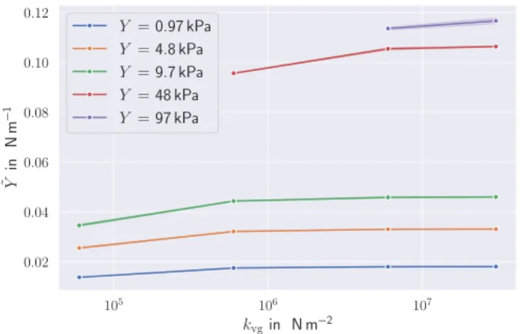
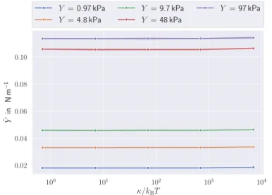
kvg to the membrane responseY˜ . . . 34 3.9 Contribution of the bending rigidity characterized byκ

to the membrane responseY˜ . . . 35 3.10 Contribution of the area constraints to the membrane

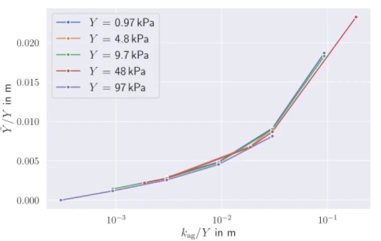
response Y˜ . . . 36

(22)

4.1 Sketch and confocal-microscopy image of cell blebbing 39 4.2 Synthetic cells consisting of a lipid-bilayer membrane

and an active actin network . . . 41 4.3 Formation of stress-induced blebs . . . 42 4.4 Schematic of the model to study cell blebbing . . . 44 4.5 Measurement of the inner network radius R over the

course of different simulations . . . 46 4.6 Comparison between the potential energies of a con-

tracting network . . . 47 4.7 Two-dimensional sketch of the interaction between the

membrane and the inner network . . . 48 4.8 Time series for different values ofC . . . 51 4.9 Blebbing transition measured through the bleb volume 53 4.10 Sketch of the relevant radii within a cell model . . . . 55 4.11 Instantaneous radiusRfor contracted cells without un-

binding (i.e k_off⁰ = 0) as a function of the contraction C . . . 57 4.12 Instantaneous radiusRas a function of the simulation

timeτfor cells with rigid membranes and different con- tractions . . . 59 4.13 Average equilibration timeτequias a function of applied

contraction . . . 60 4.14 Measured values of C_crit^meas compared to their theoreti-

cally predicted valuesC_crit^theofor rigid cell membranes . 62 4.15 Average equilibration time τequi as a function of the

applied contraction for flexible cell membranes . . . . 63 4.16 Average blebbing time as a function ofC/C_crit^theofor dif-

ferent volume constraint constantskvg . . . 64 4.17 Example cell shapes for simulated configurations with

various volume constraints . . . 65 4.18 Values of τequi for different bending rigidities κ (top)

and two shape examples (bottom) . . . 66 4.19 C_crit^meas measured against theoretical values C_crit^theo for

fixed ratioλC/kag= 38.01 . . . 68 4.20 αas a function of the ratiosλC/kagandλC/kal . . . . 69 4.21 Cell shape examples for various values of the ratioλC/kag 70

(23)

4.22 Dependence of C_crit^theo on the number of binding sites, the contraction strength λC, and the strength of the adhesion bonds λI . . . 72 4.23 Dependence of C_crit^theo on the number of binding sites,

the binding-unbinding ratioφ, and the force sensitivity FB . . . 73 5.1 Schematic of the malaria cycle within humans . . . 78 5.2 Schematic view of the merozoite during the blood stage 79 5.3 Different stages of a successful invasion event . . . 80 5.4 Examples of different membrane deformationsin vitro 81 5.5 Schematic of a RBC model . . . 84 5.6 Sketch of the different shapes used to model the parasite 86 5.7 Schematic of the vectors used to calculate the interac-

tion gradient . . . 88 5.8 Example of a parasite adhering to a RBC . . . 92 5.9 Deformation energies for the simulation shown in fig. 5.8 93 5.10 Deformation energy fora= 0and different values ofa 94 5.11 Examples for different deformation indices . . . 95 5.12 Deformation energy for different values ofa . . . 97 5.13 Examples of the adhered parasite fora= 0,1,2,3 . . . 98 5.14 Schematic of the pulling test to measure the adhesion

force . . . 98 5.15 Pulling test to measure the adhesion force . . . 99 5.16 Determination of the strain rateγ˙ . . . 100 5.17 Adhesion force as a function of the interaction strength

for the different interaction models . . . 101 5.18 Adhesion force as a function of the interaction strength

for stiffened RBCs . . . 102 5.19 Snapshots from one simulation with dynamic bond model106 5.20 Surface velocity of the parasite computed by frame by

frame analysis of in vitroexperiments . . . 107 5.21 Distributions of the surface velocities from experiments

and simulations . . . 108 5.22 Surface velocity and average number of bonds for dif-

ferent cases . . . 109

(24)

5.23 Surface velocity for different parameter sets . . . 110 5.24 Average number of bonds for different parameter sets . 111 5.25 Visualization of the head distance and angle measure-

ments . . . 113 5.26 Distribution of the head distancedfor the reference setup114 5.27 Distribution of the alignment angleθ for the reference

setup . . . 115 5.28 Alignment time for the reference configuration . . . . 116 5.29 Two dimensional probability distribution of(di, θj) . . 118 5.30 Distribution of the alignment times using MC simula-

tions for the reference configuration . . . 119 5.31 Distribution of the deformation energy for the reference

configuration . . . 120 5.32 Deformation energies for different shapes and different

values ofkoff . . . 122 5.33 Head distance distributions for different shapes and dif-

ferent values ofkoff . . . 123 5.34 Distributions of the alignment angle for the different

shapes . . . 124 5.35 Average relative alignment time for different shapes . . 126 5.36 Alignment times and deformation energies for different

ratiosk_on^short/k^long_on for short and long bonds . . . 128 5.37 Alignment time for a configuration with and without

long bonds . . . 129 5.38 Alignment times for different values ofk_on^long . . . 130 5.39 Comparison of the alignment times between rigid and

flexible RBCs . . . 131 5.40 Head distance and alignment angle for rigid and flexible

RBCs . . . 132

(25)

List of Tables

3.1 Overview of the main simulation parameters for microplate compression tests . . . 25 3.2 Comparison of the elastic constants for different levels

of mesh discretization and spring constants . . . 28 3.3 Measured Youngs’s modulus for different settings and

spring constants of elastic spheres . . . 30 4.1 Overview of the main simulation parameters for cell

blebbing simulations . . . 50 4.2 Measured values of C_crit^meas compared to their theoreti-

cally predicted values C_crit^theofor rigid cell membranes . 61 4.3 C_crit^meas measured against theoretical values C_crit^theo for

fixed ratioλC/kag= 38.01 . . . 67 5.1 Characteristic parameters of the introduced parasite

shapes . . . 86 5.2 Overview of the main simulation parameters . . . 91 5.3 Discrete deformation index to quantify the level of de-

formation . . . 96 5.4 Interaction parameters for the bond adhesion model . 105

(26)

(27)

1 Introduction

The body is a community made up of its innumerable cells or inhabitants.

Thomas A. Edison (1847 - 1931)

Cells are one of the fundamental building blocks of life. Nearly any structure and function of a living organism can be connected to one or several cells fulfilling various tasks to keep organisms homeostatic.

As a result, cells spark the interest of researchers all around the world since their first discovery by Robert Hooke in 1665 [1] till today. For example, in 2018, the Nobel price in physics was awarded for the invention of the optical tweezers and their application to biological systems [2].

The main difficulties in studying cells are their variety, complexity, and the huge number of them forming a living organism. For a human body, around 200 [3] different types of cells are known, their sizes ranging between0.1 nmand 100µm. Recent approximations suggest a total number of3.8×10¹³cells forming the whole body [4]. About 84 % of these cells are erythrocytes, also known as red blood cells (RBCs), whose main function is the transport of oxygen from the lungs to the rest of the body. On the other side, epidermal cells, which form the skin tissue, account only for about0.5 % of the total number of cells, but without them, our live would be quite different [4].

(28)

1 Introduction

1.1 Cell Structure

Cells are constructed in various ways to fulfill the vast number of tasks.

Therefore, no generic building schemes valid for all cells exist. Nev- ertheless, most cells share a number of similar features. The inside of the cell is made of cytoplasm, which consists of about 80 % water with various suspended biomolecules such as proteins and nucleic acids [5]. The cytoplasm is enveloped by a membrane that controls the entry and exit of fluids and other materials of the cell and main- tains the electric potential of the cell. The shape of cells is mainly determined by a cytoskeleton enclosed by the membrane. Depending on the cell type, this structure can be volume spanning or may only form a two-dimensional network close to the membrane. Lastly, most cells have a full copy of the genetic information stored by the DNA in a cell nucleus. Depending on the existence of the nucleus, cells are characterized as eukaryotic (with nucleus) and prokaryotic (without nucleus) cells. [5]

1.1.1 Lipid Bilayer Cell Membrane

A cell membrane mainly consists of lipids, which are amphiphilic biomolecules with a hydrophilic head group and a hydrophobic tail.

They self-organize in aqueus environments into two sheets, with their head groups pointing outwards and their tails protected from water contact, and are packed together as closely as possible (see fig. 1.1).

This lipid-bilayer forms a continuous barrier between the cytoplasm and the outside of the cell, preventing a free exchange of different materials between the outside and the inside of the cell. Within this bilayer, different membrane proteins may be embedded or attached.

[5]

The intra-membrane proteins may vary between different cell types and fulfill a variety of different tasks [7]. They are so important for the function of the cells that around30 %of the genes in an organism code for membrane proteins [8]. Common examples of these proteins

2

(29)

1.1 Cell Structure

Figure 1.1:Schematic sketch of a cell membrane. The lipids self- organize into a bilayer structure to minimize the contact of their hydrophobic tail groups with the surrounding fluids. The bilayer effec- tively separates the outside and the inside of the cell. In the bilayer sheets, a number of proteins and other biomolecules are embedded, i.e. channels, which allow a controlled exchange of ions, or receptors, which control the interaction with the surrounding environment. Pic- ture taken from [6] (open domain).

are channels and pumps, which allow for a controlled exchange of materials, such as proteins or ions. These materials may be used either as building blocks or as chemical signals within the cell, which guide the behavior of the cell. Other examples are membrane receptors, which can be used for the communication between the membrane and the extracellular space by binding certain transmitter proteins or other molecules.

Cell membranes play a vital role in the cell behavior. Membranes in mathematical and physical cell models are often represented as two-dimensional surfaces. This approach is useful, since a typical cell membrane has a thickness between5 nmand10 nm[9] and is therefore quite thin in comparison to the diameter of most eukaryotic cells. Due to the bilayer structure, cell membranes resist bending deformation,

(30)

1 Introduction

which is usually modeled by the Helfrich Hamiltonian [10] as UHelf =

ˆ

A

dA1

2κ(c1+c2−c0)²+κc1c2, (1.1) whereκis the bending rigidity of the membrane,κis the saddle-splay modulus, and A is the membrane surface area. The parameters c1

andc2describe the principal curvatures at every membrane point and c0 is the spontaneous curvature, determining the stress-free state of the membrane. The last term on the right-hand side is known as Gaussian curvature. The Hamiltonian describes an elastic energy cost to bend the membrane away from its original shape, such that these deformations require the application of external forces. Typical values ofκare in the range from of1×10⁻²⁰N mto 1×10⁻¹⁹N m[11].

1.1.2 Cell Cytoskeleton

The cytoskeleton of a cell consists of filaments and tubules of different lengths and stiffnesses [12] (see fig. 1.2). The cytoskeleton may span throughout the whole cell and is responsible for its general shape and the cell resistance to mechanical stresses [5]. Depending on cell type, other functions may be performed by the cytoskeleton, such as cell movement [15], cell signaling and the generation of cellular forces [15, 16].

The constituents of the cytoskeleton vary depending on cell type. In eukaryotic cells, the cytoskeleton generally consists of actin filaments, intermediate filaments, and microtubules. These filaments differ in size, rigidity, and function within the cell. Microtubules are stiff and hollow rods, which structurally start from a central organelle within the cell [17]. They have an average diameter of24 nm with a persistence length of a couple ofmm[18]. Microtubules are composed ofα- and β-tubulin, which self-organize in alternating, helical structures.

The incorporation of the tubulin-blocks into microtubules is dynamic and may lead to rapid growth and shrinkage behavior at the unbound

4

(31)

1.1 Cell Structure

Figure 1.2:Image of bovine endothelial cells from pulmonary arteries.

The red dye marks actin-filaments, the green color represents the microtubules, and the cell nuclei are stained blue. The cytoskeleton deter- mines the shape of the cell. The organization within the cytoskeleton varies locally, as the distinct filaments are responsible for different functions in the cell. Picture taken from ImageJ project [13, 14].

end [19]. Within the cell, microtubules function as paths for cargo transport and molecular motors [20]. They also play a vital role in the separation of chromosomes during cell division [21].

Intermediate filaments provide stability for the cell by forming a network, which absorbs mechanical stress [18, 22]. Depending on the cell type and the required functions, various kinds of structures may be formed by the filaments. Intermediate filaments are composed of protofilaments, which are bundled together forming the filament structure. They usually have a diameter of around10 nmand a persistence length on the order of hundreds ofnm[18].

The structure of cells is mainly controlled by an actin cortex, a

(32)

1 Introduction

thin network layer beneath the cell membrane (see fig. 1.2, red dye).

This layer is formed of actin filaments [16], which are built from actin monomers (G-actin) and form F-actin filaments. Actin filaments are polarized and have a double helical structure. The typical diameter is between 5 nmand 9 nmand the persistence length is on the order of tens of µm [18]. Similar to microtubules, actin incorporates its monomers by the polymerization at one end, but it also looses building blocks at the other end. This leads to a highly dynamic tread-milling behavior of the actin filaments [18]. Actin together with the molecular motor myosin plays a vital role in the generation of contraction forces, as the myosin protein is able to slide along the polarized actin filaments and generate contractile forces on the order of3 pN to4 pN[23, 24].

While the cytoskeleton and the cell membrane consist of different molecules and form distinct structures, they also interact. This membrane-cytoskeleton adhesion is usually mediated by various linker molecules, which form bonds between the constituents of both parts.

The connection is loose, such that the cell membrane is still able to move and shows membrane flickering. Additionally, the stability of the connection is sensitive to various biochemical components and mechanical stresses, which allows for structural reorganization during various cell processes. [25]

Different approaches exist for modeling of the function and mechanical effects of the cytoskeleton. These models range from detailed descriptions at the level of single protein filaments [26] to the continuous description of the cell as an elastic material [27]. Which model should be used depends on the involved lengthscales and the questions to be addressed.

1.2 Cell Deformations

One way to describe mechanical properties of cells is to use elastic constants, such as the three-dimensional Young’s modulus. For cells, typical values are in the range of 1 kPa and 100 kPa [28], which is

6

(33)

1.2 Cell Deformations

many orders of magnitudes smaller then e.g. steel with values around 200 GPa [29]. The Young’s modulus characterizes the deformability of cells, which is important for many cell functions.

Figure 1.3:Flowing RBCs in a glass tube with a diameter of7µm(A) and in a capillary with approximately the same diameter (B). While passing through the narrow channel, the cells deform drastically in comparison to their rest shape. Picture taken from [30] with permis- sion.

One example for the effect of cell deformations is the transport of oxygen by RBCs through the vascular system. The vascular system of humans consists of a large variety of vessels ranging from big arteries with a diameter on the order of a couple of mm to small capillaries with a diameter between 3µm and 10µm. The average size of RBCs is about 8µm, such that they can easily travel through large vessels. When the cells reach small capillaries, the RBCs need to deform dramatically, as shown in fig. 1.3. When the cells return to large arteries and veins again, their cytoskeletal network restores their original shape. This dynamic transition allows every cell to pass the blood circle numerous times before it is sorted out by the spleen [31].

The example of RBCs demonstrates the importance of the cell’s

(34)

1 Introduction

mechanical properties and a number of techniques are available to measure quantities such as Young’s modulus and other mechanical characteristics. These techniques can be divided into two classes: direct force application and force sensing methods [32].

Force application techniques exert external stresses to deform cells and derive their elastic properties by interpreting the cell reaction.

The applied forces can be of various types, e.g. mechanical stress using atomic force microscopy [33–37]. Other methods utilize optical techniques (optical tweezers [38–42], optical stretcher [43–46]), magnetic and/or electric stimulation (magnetic tweezers [47–50], electric field stimulation [51, 52]), or acoustic approaches (acoustic tweezers [53–55]). To study cells in flow environments, a number of flow techniques are available [56–64]. For example, in microfluidic devices, cells are deformed by flow stresses and through the interaction with geometrical boundaries such as shown in fig. 1.3.

Force sensing techniques focus on forces that are a result of internal cell processes. Examples are cell motility and reorganization during cell division. A number of methods such as optical tweezers and atomic force microscopy may also be applied within the force sensing context [32].

The interpretation of experimental results often requires models to quantify the elastic properties. Experimental measurements of cell mechanics may be too complex to be reliably quantified by analytical models, such that computer models and simulations are required for interpretation. The resulting field of computational physics can be placed between the experimental and theoretical branches of physics and plays an important role in ongoing research.

1.3 Thesis Structure

In this thesis, a number ofin silicomodels are employed to study various aspects of cell-membrane deformations and adhesion. In particu- lar, we identify the physical mechanisms leading to stress-induced cell

8

(35)

1.3 Thesis Structure

blebbing and the RBC deformations through the adhesion of malaria parasites.

In chapter 2, a short introduction into the broad field of computational physics is given. We present two simulation frameworks, dissipative particle dynamics [65] and Brownian dynamics, which allow the modeling of hydrodynamic interactions and cell mechanics.

A cell model is introduced in chapter 3. Cells are described by a number of simulation particles, which represent a volume-spanning cytoskeletal network and a lipid-bilayer cell membrane. The elastic properties of the cell are quantified by simulating cell compression by microplates [66]. We investigate the effect of different membrane and cytoskeleton parameters on the total cell deformation and show that the elastic response of the cell is a superposition of the inner network and membrane responses.

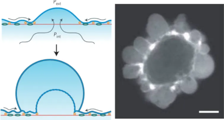
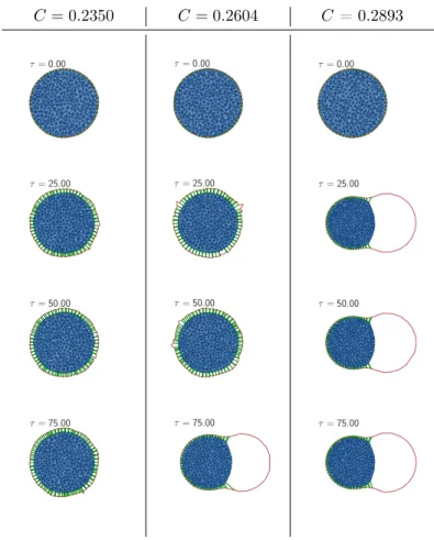
Cell blebbing is a common cell phenomenon occurring in various processes such as cell motility and cell death [67–73]. A bleb is a cell membrane protrusion, which appears when membrane and cytoskeleton disconnect locally. Blebbing may occur due to different mechanisms, one of which is stress-induced cell blebbing. Here, the active contraction of an actin network by myosin motors leads to blebbing [74]. In chapter 4, stress-induced cell blebbing is studied. We extend the cell model by adding network contraction and a dynamic membrane-cytoskeleton adhesion [25, 75]. By quantifying the effects of various parameters, we obtain criteria for the existence of stress- induced cell blebbing.

Another biological process considered in this thesis is the adhesion of malaria parasites to RBCs. Malaria is caused by parasites, which employ RBCs to progress through various stages of a complex life cycle and ensure their survival [76]. The invasion of human RBCs by parasites is an important step in this cycle. Before the invasion, parasites interact with a targeted RBC and induce various levels of deformation of the cell membrane [77–86]. We study the pre-invasion stage of malaria parasites with a cell membrane model of a healthy RBC in chapter 5. The RBC interacts with a parasite through an ad-

(36)

1 Introduction

hesive interaction, which is either represented by an attractive potential interaction model or by a bond-based, dynamic adhesion model.

The models are used to investigate the passive compliance hypothesis, which explains the membrane deformations purely by mechanical interactions [86].

10

(37)

2 Simulation Methods

Physics is a broad field that aims to explain a wide range of phenom- ena, starting from the movement of the stars and planets within the universe to the mechanics of the smallest particles that form this universe. Clearly, these problems have different length- and timescales

Å nm μm mm m

fs ps ns μs ms s min

h

Distance Time

Quantum Mechanics

Molecular Mechanics

Mesoscale Modeling

Continuum Mechanics

Figure 2.1:Overview of length- and timescales in the realm of physics.

Over the last decades, a number of different theoretical and computational descriptions and methods have been developed to tackle the problems involving the various scales.

and their investigation requires different approaches (see fig. 2.1).

Therefore, a multitude of different methods have been developed to tackle them. One type of approach are numerical simulations, where

(38)

2 Simulation Methods

complex mathematical models employ the capabilities of modern computers.

For solving different mathematical problems, a variety of computational methods exists, e.g. finding roots of an equation or solving large systems of linear equations. In this thesis, we focus on advanced computer simulations, which are used to study complex systems with a large number of components, e.g. the number of elements in a cell membrane or a fluid. These simulations are generally classified into particle-based and continuum-based simulation techniques. In particle-based simulations, the studied system is discretized into a number of particles that interact with each other. These particles may e.g. represent molecules or small molecular structures, leading to the method of molecular dynamics (MD) simulations. The complexity of MD simulations results from the large number of degrees of freedom representing atomic and molecular structures and therefore MD simulations are often used to study relatively small length- and timescales. Several examples of MD simulations can be found in references [87–93].

Problems at large scales are generally studied with continuum simulation methods. Such methods, e.g. finite elements methods (FEM), utilize partial differential equations (PDEs), such as the Navier-Stokes equation for fluid flow. PDEs are usually discretized by dividing the space into smalls elements (finite elements) and approximating the equation locally at these elements resulting in a numerical solution for the studied system. Examples of continuum methods can be found in [94–98].

Biophysical problems mostly evolve around cells, their constituents and the networks they form. Cells have different shapes and sizes in the range from 1µm to 100µm; thus they are best described by mesoscopic models. At cellular lengthscales, physical models have to address an interesting mix of different problems. On the one hand, the number of atoms, which form a single cell, is too high to model cells with atomistic representation using molecular dynamics. There- fore, one has to average out a large number of these atoms to obtain

12

(39)

2.1 Dissipative Particle Dynamics

manageable systems, which reproduce the properties of cells. This process, known as coarse-graining, is a vital step in the establishment of mesoscopic models. On the other hand, supra-molecular, cellular structures such as membranes are important to capture cell mechanics. Therefore, we need to be careful while averaging, such that this essential information is not lost during coarse-graining. Hence, the level of coarse-graining generally depends on the problem of interest and questions addressed.

Cell cytosol is generally represented by a fluid environment. At the same time, cells are suspended into some fluid medium. Therefore, a typical cell simulation includes required structural elements of a cell to represent cell mechanics and two fluids (i.e. cytosol and suspending medium) separated by the cell membrane. A number of simulation techniques have been established to study this type of system, such as multi-particle collision dynamics (MPCD) [99, 100]), smoothed particle hydrodynamics (SPH) [101–104], and Lattice Boltzmann methods (LBM) [105–108]. In this chapter, we introduce the dissipative particle dynamics (DPD) framework, where hydrodynamic effects are modeled by fluid particles, and the Brownian dynamics (BD) framework, which incorporates fluid interactions implicitly. In the following chapters, a number of different cell models are presented, which employ these fluid methods.

2.1 Dissipative Particle Dynamics

To model hydrodynamic interactions, the framework of DPD is used.

In DPD, the fluid is modeled by a number of particles and each particle is described by its position r_i, velocityv_i, and massmi. These particles represent small volumes of the fluid; thus the number of particles is much smaller than the number of molecules. The amount of simulation particles is described by the number densityρ. The fluid particles interact by a pairwise force

F_ij =F^C_ij+F^D_ij+F^R_ij (2.1)

(40)

which conserves the linear and the angular momentum of the fluid [109]. We follow the standard implementation by Español [65] to describe these forces.

The term F^C_ij is a soft, repulsive conservation force that prevents particle overlapping and is given by the relation

F^C_ij=w^C(rij)eij, (2.2) whererij=ri−rjis the distance vector between the particlesiandj, rij =|ri−rj|andeij =rij/rij. The functionw^Cis a weight function and is modeled as a decaying function

w^C(rij) = (aij

1−^rr^ijc

rij ≤rc

0 rij > rc

, (2.3)

whereaij is the interaction strength andrc is the cutoff radius of the interaction. Their values are chosen to ensure incompressibility of the modeled fluid. They depend on the number densityρand the thermal energykBT of the system.

The forceF^D_ij models the fluid viscosityη by introducing a dissipative force and the termF^R_ij models the effects of thermal fluctuations.

They are given by

F^D_ij=−γw^D(rij) [vij·eij]eij, (2.4) F^R_ij=σw^R(rij)θijeij, (2.5) where γ is a friction constant and σ is the coefficient of the random force. The vector vij = vi −vj is the velocity difference between the particles. The random component of F^R_ij isθij. It models Gaus- sian white noise that is symmetric in i and j to ensure momentum conservation. It fulfills the relations

hθij(t)i= 0, (2.6)

hθij(t)θkl(t⁰)i= (δikδjl+δilδjk)δ(t−t⁰). (2.7)

14

(41)

2.1 Dissipative Particle Dynamics

To obtain detailed balance, the weight functions need to satisfy w^D(r) =

w^R(r)²

. (2.8)

Then the version of the fluctuation-dissipation-theorem in DPD becomes

σ²= 2γkBT /m, (2.9)

which connects the friction and random contributions to the thermal energykBT. The weight function is given by

w^D(rij) =

w^R(rij)²

=





 1−^rr^ij_c

^k

rij ≤rc

0 rij > rc, (2.10) similar to the weight function of the conservative force. The additional exponent k is used to control the viscosity of the fluid, wherek = 1 reproduces the original DPD algorithm [110].

The time evolution of one DPD particlexis determined by Newton’s second law of motionm¨x=F, whereFis the sum of all forces acting on the particle. Since each particle is influenced by its neighbors, the particle trajectory is obtained by numerical integration using the verlet algorithm, which is given by the equations

x(t+ ∆t) =x(t) + ˙x(t) ∆t+1

2x¨(t) ∆t², (2.11)

˙

x(t+ ∆t) = ˙x(t) +1

2[¨x(t) + ¨x(t+ ∆t)] ∆t, (2.12) where the timestep∆tis selected.

2.1.1 Measurement of Fluid Viscosity

An important property of a fluid is the viscosityη. In the DPD framework, it depends on the interaction parametersγ, a, k, the thermal

(42)

F

F vy

Figure 2.2: Sketch of the reverse Poiseuille flow setup. The simulation box is divided into four parts. A constant force is applied to each particle, the direction of the force alternating between the parts. The resulting parabolic flow profile is sketched by the red line. The dash line indicates periodic boundary conditions.

energy kBT, and the number densityρ of DPD particles. η is measured using a Poiseuille flow setup, as shown in fig. 2.2. The simulation box is divided into four parts in the x-direction. A constant force is exerted on all particles, but its direction alternates between the four simulation parts, as indicated by the arrows in fig. 2.2. We choose a division into four parts to guarantee the development of the flow profile at the inner lines without interference of the applied boundary conditions.

The resulting flow profile for each of the four parts is derived from the Navier-Stokes equations and is given by

vy= F ρ

2ηx(H−x), (2.13)

where vy is the velocity in the direction of the applied force, x is the position within the box, and H is the width of each of the four simulation parts. To reduce effects of the applied boundary conditions, the profile is only measured in the two boxes in the middle of the setup.

[111]

16

(43)

2.2 Brownian Dynamics

The DPD framework allows a high level of coarse-graining, therefore reducing the computational cost to model a fluid dramatically in comparison to a fully atomistic description. Nevertheless, the amount of computational cost might still be very high for a hydrodynamic representation. Therefore the BD method is introduced. It incorporates friction and thermal effects implicitly without explicitly modeling the fluid particles, thus significantly reducing the computational effort at the cost of loosing the effects of momentum transfer within the fluid.

At the core of the BD method is again Newton’s second law of motion for the simulation of particles. These particles may represent e.g.

the constituting particles of cell membranes, which will be introduced in the next chapters. For a particle with positionx, the equation of motion is given by

m¨x=−γx˙ +p

2γkBTR(t) +FI. (2.14) This equation is known as the Langevin equation. The first term on the right-hand side introduces a dissipative force with the friction coefficientγ. The second term models thermal fluctuations governed by the thermal energy kBT. The random component R(t) models Gaussian white noise, which fulfills the relations

hR(t)i=0, (2.15)

hR(t)R(t⁰)i=δ(t−t⁰). (2.16) In contrast to the DPD method, the random contribution is orientated arbitrary in space and not parallel to the distance vector between two particles. The last termFI represents all other interactions that act on the simulation particles.

To obtain the BD method from the Langevin equation, we can as- sume the overdamped limit i.e. m¨x = 0, which is a realistic as- sumption in biological systems. The obtained dynamics becomes

(44)

purely diffusive, if no other interactions are introduced. The Einstein- Smoluchowski relation defines the diffusion constant of a particle as

D=kBT /γ. (2.17)

Furthermore, the friction coefficient is connected to the viscosity of the implicitly modeled fluid through the Stokes equation as

γ= 6πηa, (2.18)

where η is the viscosity andais the effective radius of the simulated particles. To obtain the dynamics of the particles, these equations of motion are integrated in time by the Verlet algorithm.

The BD framework can be used for simulations, in which the dissipation within the fluid plays a vital role, but other hydrodynamic effects can be neglected.

2.3 Simulation Units

Parameters in numerical simulations are selected in simulation units.

A number of scales may be defined, allowing to connect the simulation values to the physical parameters. In general, energy-, length- and timescales are required.

Let E be a simulation parameter with the dimension of energy.

For soft matter problems, a well established energyscale is the thermal energykBT. The connection of the simulation parameters to the physical values is done through the dimensionless quantity

E^M

(kBT)^M = E^P

(kBT)^P, (2.19)

where the superscript ^M denotes a simulation parameter and ^P the physical values. The physical value of Eis then obtained by

E^P = (kBT)^P

(kBT)^ME^M (2.20)

18

(45)

2.3 Simulation Units

where only the physical quantity (kBT)^P needs to be known. For example(kBT)^P = 4.282 pN nmfor experiments at room temperature.

In the same way, lengthscaling is established as x^P = D^P₀

D^M₀ x^M, (2.21)

wherexis a value with the dimension of length andD0is a characteristic lengthscale. For cell simulations, the average cell diameter can be used for this purpose. Timescaling may be achieved by combining energyscale, lengthscale, and the viscosity η of surrounding fluid to obtain

t^P = η^P η^M

D^P0

³ D^M₀ 3

(kBT)^M

(kBT)^Pt^M. (2.22) Using the fundamental scales of energy, length, and time, other quantities can be calculated. The physical values of a force F are found as

F^MD^M₀

(kBT)^M = F^PD₀^P

(kBT)^P, (2.23)

F^P = D0^M

D^P₀

(kBT)^P

(kBT)^MF^M. (2.24) This scheme is easily adapted for other quantities of interest.

In this thesis, both simulation and physical values will be used.

If not stated otherwise, a quantity given in physical units refers to a transformed value as described above. If a value is given without physical dimension, it refers to a simulation or model value.

(46)

(47)

3 Cell Model

Cells fulfill a variety of tasks within any living body. Consequently, this diversity of functions and environments requires a similar amount of models to study cells (see fig. 3.1). Cell models may be divided into two major categories, which depend on the required resolution of the studied cell. Micro- and nanostructure models focus on the cytoskele-

Mechanical models for living cells

Continuum Approach Micro/Nanostructural

Approach

Viscoelastic models Biphasic model

Cortical shell-liquid core models - Newtonian - Compound - Shear thinning

- Maxwell

Solid Models - Elastic - Viscoelastic

Fractional derivative model - Power law structural damping

Cytoskeletal models for adherent cells - Tensegrity model - Tensed cable

networks - Open-cell foam

model

Spectrin-network model for erythrocytes

Figure 3.1:Selection of different types of models to study the properties and behavior of various cells [112–118].

tal and single filament contributions toward the cell mechanics. The developed models have been used extensively to study the mechanics of adherent cells (see [112–116]). Continuum models neglect these characteristics and treat cells as comprised material with continuous mechanical properties such as Young’s modulus and Poisson’s ratio.

(48)

3 Cell Model

These properties are derived using experimental methods and allow an effective description of bigger cell systems [118].

The particle-based cell model introduced in this chapter may be counted as a continuous cell model, where we coarse-grain the studied biological system to obtain a tractable model, that can represent whole cells on available computers. Thus, in the introduced systems, each particle does not represent single molecules or filaments, but models a discrete area or volume of a cell with homogeneous average properties of that area or volume. A drawback of the coarse-graining process is the loss of information at smaller scales. Therefore, effective potentials need to be introduced to mimic cell properties.

The aim of this chapter is to derive a coarse-grained cell model that incorporates properties of a bulk cytoskeleton and a lipid-bilayer membrane with underlying cell cortex. The model is used to study how applied mechanical stresses induce deformations of complex, cellular structures. To this end, the deformation of different structural elements of the cell is studied using a microplate compression setup. The results supply information about the interaction between cell membrane and bulk cytoskeleton.

3.1 Bulk Cytoskeleton

The usage of a coarse-grained modeling approach allows us to neglect the details of different fibers, which form a cytoskeleton and model it as an elastic, random mesh network. This network consists of a number of vertices N that are distributed within a volume V. The vertices are connected by NS springs, which are established between direct neighbors. The network templates used in our simulations are created using TetGen [119].

The springs correspond to a harmonic potential that is given by Unetwork({li}) =X^NS

i=1

λ

2 li−l_i⁰²

, (3.1)

22

(49)

3.1 Bulk Cytoskeleton

whereliis the instantaneous length of the springiandl⁰_i is the corre- sponding rest length. The valueλis the spring constant, characteriz- ing the strength of each spring. The model is implemented within the BD framework, which represents thermal fluctuations and dissipation from an implicit fluid.

The cytoskeletal material is assumed to be isotropic and its me- chanic properties are described by two elastic constants. Using elastic theory, the values of Poisson’s ratio ν and the bulk modulus K are established as

ν =¹/⁴, (3.2)

K=1 9

NS

V Dλ l⁰i

²E

. (3.3)

The value ofν shows that the elastic network is compressible. Other elastic constants can be derived from ν and K. For example, the elastic or Young’s modulus is given by

Y =1 6

NS

V Dλ l⁰i

2E

. (3.4)

All mechanical properties can be calculated through the properties of the mesh as well as the spring constant. [120, 121]

3.1.1 Microplate Compression Setup

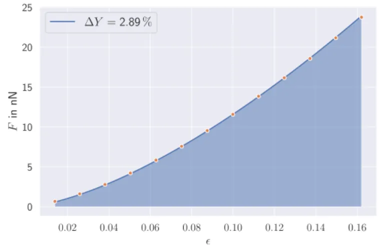
The elastic material properties are measured by performing microplate compression testsin silico [66, 122]. The modeled material is put between two rigid plates, as sketched in fig. 3.2. The upper plate is moved down toward the material with a constant velocity, leading to deformation. The engineering strain is used to quantify the deformation. It measures the relative change in height∆D with respect to the initial heightD0:

= ∆D

D = D0−D D0

. (3.5)

(50)

3 Cell Model

-5.0 -2.5 0.0 2.5 5.0

xinµm 0.0

2.5 5.0 7.5 10.0

zinµm

-5.0 -2.5 0.0 2.5 5.0

xinµm 0.0

2.5 5.0 7.5 10.0

zinµm

Fcompress

Figure 3.2: Sketch of a microplate compression experiment for a spherical elastic particle. The particle is put between two plates and the upper plate is moved down with a constant velocity. The induced deformation of the network is quantified by the engineering strain. Due to the elasticity of the material, the reaction forceFcompress is obtained.

The microplates are represented by rigid walls, which interact with the deformed particle using the repulsive part of the Lennard-Jones (LJ) potential:

Uwall(r) = 4LJ

σ r

¹²

−σ r

⁶

, r≤√⁶

2σ. (3.6) The potential acts between the wall and the vertices of the network.

A large value for the interaction energyLJ and a small value for the characteristic lengthσare chosen to ensure a hard wall approximation.

The LJ potential is also used to measure the reaction forceFcompress, as the particle resists the induced deformation. The force is calculated by summing all force contributions in the compression direction from the vertices within interaction range. To overcome the effects of thermal noise, the simulation is divided into compression and measurement parts. During the first part, the cell is compressed, while during

24

(51)

3.1 Bulk Cytoskeleton

the second part, the strain and the force Fcompress are measured.

This allows averaging over a long enough time period, leading to reliable results. At the same time, the information about time evolution is not considered, so that no timescales are used in the simulations.

3.1.2 Comparison Between Theory and Simulation

A number of simulation parameters are required to perform the microplate compression tests. The main parameters, that are constant for all simulations performed in this chapter, are summarized in table 3.1.

Parameter Simulation Value Physical Value kBT 0.0001 4.282×10⁻²¹J

D0 10 10×10⁻⁶m

γ 50

∆t 0.005

Table 3.1:Overview of the main simulation parameters for microplate compression tests. The thermal energykBT and the average size of a particleD0 are used as energy- and lengthscales. γandkBT are required to use the BD framework. A timescale is not used on the simulations, as only quasi-static deformations are studied.