Targeting REP:GGTase-II interaction and finding new means to predict the protein:ligand interactions

Targeting REP:GGTase-II Interaction and Finding New Means to Predict the

Protein:Ligand Interactions

DISSERTATION

zur Erlangung des akademischen Grades Doktor der Naturwissenschaften

(Dr. rer. nat.)

vorgelegt von

Mahesh Kulharia B.Sc., M.Sc. in Biotechnology,

aus Hissar, India

eingereicht bei der Fakultät Chemie

der Technische Universität Dortmund

Erstgutachter: Prof. Dr. Alfons Geiger

Zweitgutachter: Prof. Dr. Roger Goody

Dritter Prüfer: Prof. Dr. Martin Englehard

CONTENTS Contents

Symbols and Abbreviations Acknowledgements

1.0 Introduction

i iv

v 1 1.1 General Background

1.2 Computer aided drug design

1.3 Protein-protein interactions: General aspects

1.4 Protein-protein contacts: Composition and nature of interactions 1.5 Thermodynamics and kinetics of protein-ligand interactions 1.6 Scoring functions

1.7 Molecular mechanics-based scoring functions 1.7.1 Bonded energy terms

1.7.2 Non-bonded energy term 1.8 Empirical scoring functions

1.9 Knowledge-based scoring functions

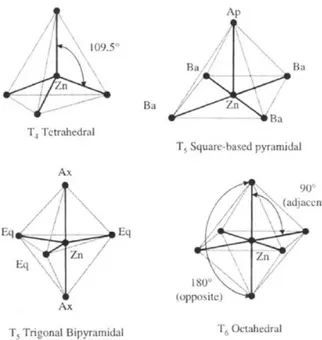
1.10 Treatment of divalent ions (such as zinc) in scoring function 1.11 Virtual screening

1.12 Docking and scoring

1.13 Predicting Ligand binding sites 1.14 Predicting protein-ligand affinity 1.15 Aims and objectives

1.16 Thesis outline

2.0 Structure-based pharmacophore design and targeting REP- GGTase-II interaction interface

1 2 2 3 3 4 5 5 6 7 8 9 10 11 12 14 16 17 21 2.1 Abstract

2.2 Introduction

2.3 Biological perspective

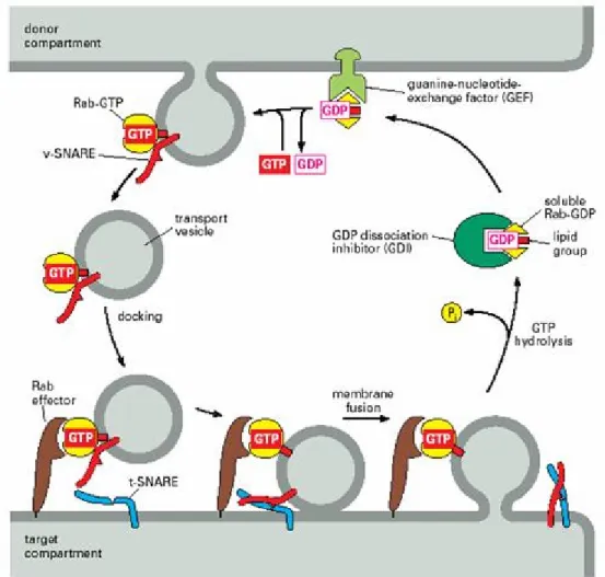
2.4 Understanding the enzyme system of Rab prenylation 2.4.1 Rab proteins

2.4.2 GGTase-II

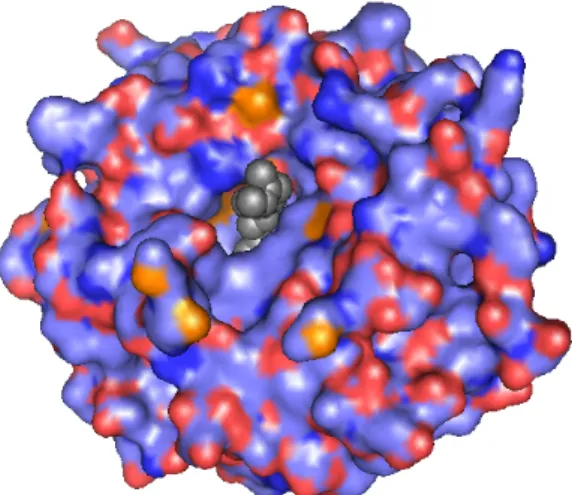
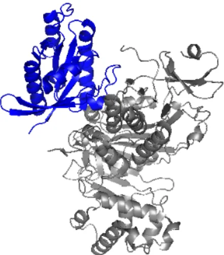
2.4.3 Rab Escort Protein 2.4.4 Rab-REP interface 2.4.5 REP-GGTase-II interface 2.5 Targeting the enzyme system 2.5.1 Putative targets in enzyme system 2.5.1.1 Ligand binding sites

21

22

23

24

24

25

28

29

30

33

33

33

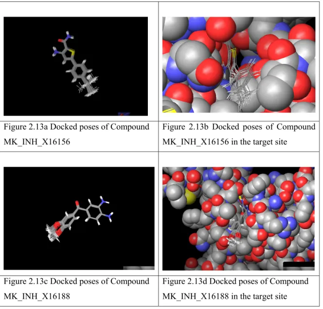
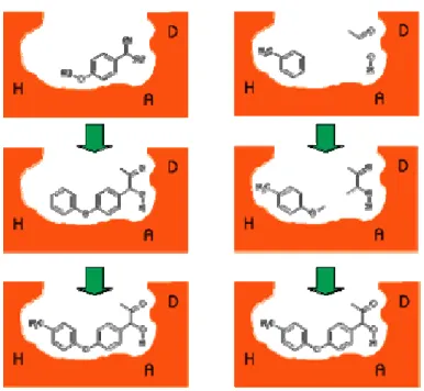
2.7.2 Docking based identification of stable “anchor” fragment for growing molecules

2.7.3 Molecules generated by growing the guanidine tail

2.7.4 Diversification of the hydrophobic part of lead_molecule_1;

Pharmacophore generation; Virtual screening and Assay results 2.8 Conclusions

2.9 References 2.10 Appendices

3.0 InCa-SiteFinder: A method for structure based prediction of carbohydrate binding sites on proteins

37 38 39 41 43 45 51 3.1 Abstract

3.2 Introduction 3.3 Methods

3.3.1 Construction of dataset for propensity calculation 3.3.2 Calculation of amino acid propensities

3.3.3 InCa-SiteFinder

3.3.4 Definition of a true carbohydrate binding site 3.3.5 Optimisation of InCa-SiteFinder performance 3.3.6 Calculation of sensitivity and specificity 3.3.7 Optimisation of InCa-SiteFinder

3.3.7.1 Determination of PSSBC cut-off for classifying a region as a site 3.3.7.2 Determination of differential propensity score cut-off for carbohydrate binding site

3.3.8 Dataset for evaluation of the ability of the InCa-SiteFinder to

distinguish between the carbohydrate binding sites and drug-like compound binding sites

3.4 Results and discussion

3.4.1 Amino acid propensity to interact with carbohydrate molecule 3.4.2 10-fold cross-validation and optimisation of InCa-SiteFinder 3.4.3 Validation of optimised InCa-SiteFinder

3.4.4 Determination of PSSBC cut-off value

3.4.5 The importance of differential propensity score for the recognition of carbohydrate binding sites

3.4.6 Evaluation of DPS and threshold values 3.5 Some examples of site prediction 3.6 Conclusions

3.7 References 3.8 Appendices

51

52

54

54

54

55

57

57

58

59

59

60

60

61

61

62

65

66

66

68

69

71

73

76

4.0 An Information theory-based scoring function for the structure- based prediction of protein-ligand binding affinity

4.1 Abstract 4.2 Introduction 4.3 Methods

4.3.1 Construction of an atom pair contact database 4.3.2 Calculation of atomic contact preferences

4.3.3 Generation of a protein-water contact database and atomic solvation- desolvation measures

4.3.4 Protein-ligand test set 4.4 Results

4.4.1 Choice of scoring function 4.4.2 Choice of scoring parameters

4.4.3 Inclusion of Solvation effects and SIScoreJE 4.4.4 Comparison of different scoring functions 4.4.5 Identification of Near-Native Configurations 4.5 Discussion

4.6 Conclusions 4.7 References 4.8 Appendices

5.0 Conclusion Future Perspectives

80

80

81

83

84

88

89

89

90

90

92

94

98

99

101

103

104

107

113

115

Symbols and Abbreviations

Å Angstrom

CADD Computer Aided Drug Design CBP Carbohydrate Binding Propensity DPS Differential Propensity Score GDP Guanosine Diphosphate GGpp Geranylgeranyl Pyrophosphate GGTase Geranylgeranyl Transferase GTP Guanosine Triphosphate

HBA Hydrogen Bond Acceptor HBD Hydrogen Bond Donor IC50 Inhibition Concentration 50%

InCa Inositol-Carbohydrate LBDD Ligand-based Drug Design M Molar

nM nano Molar

NI Negative Ionisable

PSSBC Propensity Score of a Site to Bind Carbohydrates PSSBnC Propensity Score of a Site to Bind non Carbohydrates PI Positive Ionisable

RBP Rab Binding Platform REP Rab Escort Protein ScoreJE Score Joint Entropy

SIScoreJE Solvation Included Joint Entropy

SBDD Structure-based Drug Design

Acknowledgements

I would like to take this opportunity to convey my heartfelt thanks to the following people,

Prof. Roger Goody for sharing my problems and extending care and rock-solid support in times of need. His unwavering support has been an immense source of strength and hope.

Prof. Alfons Geiger for listening to my presentations and the valuable advice and guidance he provided during PhD.

Prof. Martin Englehard for taking out time to view my project work and for the kind words of support and encouragement.

Dr. Richard Jackson for burning midnight oil in helping me to realise the objectives we had set.

Dr. Alexey Rak and Dr. Olena Pylypenko for the help they extended in the initial stages of my work.

Prof. David Westhead for asking questions and giving good advice when needed.

I am grateful to my father, brother and wife Sarita for being there in times of rough sea.

Thanks Nagaraj and Gurpreet Singh for listening to my daily quota of ideas and giving me valuable advices on feasibility of some of the projects; Amit Sharma and Parbhu Dayal Jakhar for being close to my family in times of need. Harry Mathala for helping me with programming and providing me insights of molecular modelling.

Dr. Tetsuya Kitaguchi, Dr. Anne Adida, Dr. Sergei Mureev (Captain Barbossa) and

Chapter 1: Introduction

1.1 General Background

Drugs are single or combinations of small molecules with defined composition and specific pharmacological effect. The process of identification of new drugs is regulated by legal agencies like “Food and drug administration”. This process can be divided in to the phases of drug discovery and drug development. Drug discovery process involves the application of different conceptual strategies to obtain novel protein activity modulators, deduction of the mechanism of these compounds, lead demonstration and optimisation, in vivo proof of concept and simultaneous demonstration of a therapeutic index. Drug development begins when the drug molecule is put in phase I clinical trials.

On an average the time from conception of the targeting strategy to the grant of

approval by a regulatory authority for a new drug molecule is 10-15 years. It is estimated

majority of drug candidates fail along the way. This results in huge loss for consumers

(pharmacy companies pass their loss to patients) as the cost of bringing a new drug to

market is close to a billion dollars (Dimasi et al, 2000). Hence the a number of approaches

have been adopted to help distinguish the druggable targets from non-druggable ones. One of

the major goals of computational chemistry, or the rational design of compound libraries, is

to maximise diversity, to enhance the potential of finding active compounds in the initial

rounds of virtual screening programs. Drug discovery has traditionally required testing of

hundreds of individually synthesized and characterized chemicals; the new techniques of

virtual synthesis in computational chemistry, and virtual screening (VS) offer the possibility

of rapidly preparing and examining hundreds of compounds. This increased screening ability

dramatically increases the probability of finding a lead compound with the proper balance of

activity, specificity, safety, bioavailability, and stability to result in a successful new drug.

1.2 Computer-Aided Drug Design

Computer-Aided (Assisted) Drug Design (CADD) is a generic term used to address various computer-based drug design strategies. This field can broadly be divided into two categories (1) Ligand-Based Drug Design (LBDD) exploiting information of known actives and (2) Structure-Based Drug Design (SBDD) carried out in the presence of a protein structure. The important background relating to protein-ligand interactions is discussed below. Since the application of computational techniques have the objective of designing the small molecules and this we designed inhibitors for the disruption of REP:GGTase-II interaction, the general aspects of protein-protein interaction followed by concepts in current understanding about kinetic and thermodynamic aspects of protein-ligand binding are discussed. The general methods used in the process of CADD are discussed next i.e. virtual screening (VS), docking, and de novo drug design.

1.3 Protein-protein interaction: general aspects

Protein-protein interaction is the fundamental process for the functioning of the huge

number of processes in the living cells. Malfunctioning of any part of protein turnover

machinery can cause occurrence of non-native interactions that may lead to pathological

disorders such as Alzheimer’s disease. The regulation of protein-protein interaction is

mediated either through control of external conditions (such as pH and ionic strength) or by

the activity of other cellular proteins (example enzymes). An important feature of protein-

protein interaction is the variety in their interaction modes. The types of pits, grooves, voids

and pockets that can possibly be generated by the arrangement of amino acid side chains are

extremely diverse. Current approach for rational drug design involves the targeting the active

sites in a protein which leads to broad spectrum of effects. Moreover the targeting of enzyme

active sites by this approach is under effective as the mutations in active site coupled with

the cellular process have an inbuilt redundancy and alternative pathways generally can compensate the inhibition. In addition the knowledge about any starting compound for the inhibitor design is not straight forward as unlike the enzymes there is no small molecular substrate.

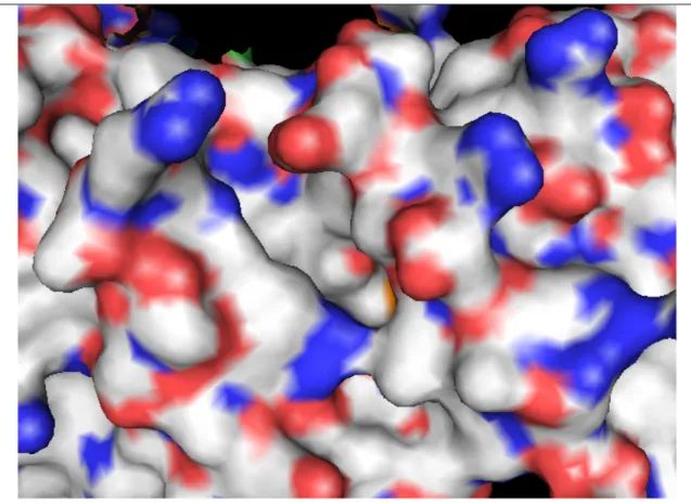
1.4 Protein-protein contacts: Composition and nature of interactions

Protein-protein interactions typically bury 1600Å ² of the surface area at the interface (Buckingham, 2004). The interface is potentially rich in arginine, histidine, asparagine, tryptophan, tyrosine and serine (Davies, D.R. et al, 1996). Analysis of secondary structures in the interface areas showed that the random coil comprises 47% of the protein-protein interaction interface; 36% α-helix; 17% β-sheet (Nissinov, R 1997). The interaction forces are van der Waals, hydrophobic and electrostatic in nature. The degree of surface complementarity between interacting interfaces is dependent on the strength of complex.

Permanent complexes interfaces have a high surface complementarity whereas temporary complexes have less interfacial complementarity. (Jones S et al 1996).

1.5 Thermodynamics and kinetics of protein-ligand interactions

Protein-ligand interactions can be experimentally measured under thermodynamic equilibrium conditions from which the inhibition constant K i can be obtained (Equation 1.2).

The inhibition (or dissociation) constant describes the strength of protein-ligand binding as

mole/l. A ligand binds stronger to the receptor when the K i is small (e.g. nanomolar). If there

is less ligand present than the value of K i, then only a small proportion of the protein will be

associated with the ligand and a biological effect may be difficult to measure. IC 50 term gives

the ligand concentration at which the enzyme activity decreases to 50%. It is shown that both

IC 50 and K i characterise protein-ligand interactions in a similar way, so that the easily

(ΔH˚) and entropic contributions (TΔS˚) which can be measured experimentally by Isothermal Titration Calorimetry (ITC) or van’t Hoff analysis (Holdgate and Ward, 2005).

These experiments have shown that ΔG˚ and ΔH˚ are not directly correlated, thus enthalpy alone is not an adequate measure for binding affinity (Boehm and Klebe, 1996). Receptor [R] and ligand [L] associate and form a non-covalent, reversible receptor-ligand complex [LR] in solution under thermodynamic equilibrium conditions.

] [ ] [ ]

[ R + L ↔ RL 1.1

The experimentally determined inhibition constant (K i ) or dissociation constant (K D ) or reciprocal association constant (K A ) describes the relationship between bound and unbound molecules.

] [

] ][

[ 1

RL L R K K

K

A D

i = = = 1.2

The Gibb’s free energy of binding (ΔG˚) comprises an enthalpic (ΔH˚) and an entropic term (TΔS˚) where T is the temperature in Kelvin and R is the gas constant (1.987 cal /(K mole)).

ΔG˚ = -RT ln K A = RT ln K i = ΔH˚ - TΔS˚ 1.3

1.6 Molecular mechanics-based scoring functions

Computational methods such as docking are applied to identify the correct orientation

of the ligand in the binding site and estimate ligand binding affinities. These docking

protocols comprise of an algorithm for searching the conformational space to identify the

most probable orientation of a molecule in the binding pocket and a scoring function which

based functions (e.g. ChemScore, X-Score) or (3) knowledge-based potentials (e.g. PMF, DrugScore). These different types of scoring functions will be reviewed in the following sections.

1.7 Molecular mechanics-based scoring function

Molecular Mechanics (MM)-based scoring functions (also termed force field or first principle based methods) approximate binding affinity by summing individual contributions in a master equation. The terms used for different interaction types are based on physicochemical theory and should not be cross correlated with each other. These terms are often combined with solvation and entropic terms.

An example in terms of docking is the original DOCK 3.0 score (Meng et al., 1992). It is one of the earliest scoring functions and covers the principal contributions to binding: shape and electrostatics accounted for in terms of a van der Waals term and an electrostatic potential term. These separable terms are combined into a grid-based AMBER force-field scoring function which is computed at specific grid points according to the field generated by the receptor. The overall score is then calculated as the sum of ligand atom interactions at the grid points (using a interpolation scheme) assuming additivity of individual terms (Tame, 1999).

In contrast to time-consuming quantum mechanics methods, that describe molecules based

on their electron distribution by ab-initio or semi-empirical approaches, force fields or

molecular mechanics describe molecules reduced to their atoms and bonds i.e. as charged

atom centres, with masses assigned according to atomic weight connected by springs. They

usually comprise two energy components, one for the protein-ligand interaction and another

for the internal (conformational/strain) energy of the ligand (and sometimes the protein). The

protein conformational energy is often left out as usually only a single conformation is

considered during docking. MM-based scoring methods most often assume a common

Potential Energy = E bond + E angle + E dihedral + E elec + E vdw

(bonded) (non-bonded) 1.4

The total energy of a conformation comprises several energy terms (Brooks et al., 1983).

1.7.1 Bonded energy terms

The bonded energy terms comprise the bond (E bond ), bond angle (E angle ), dihedral (E dihedral ) and improper torsional potentials (E impr ), all together referred to as the bonded interactions (Equation 1.5). The bond and angle deformations (E bond , E angle ) are generally small. As such, deviations from equilibrium bond and angle values are treated with large energy penalties. The dihedral angle is defined by four atoms, with the torsion angle about the axis of the middle pair of atoms. The improper torsion potential is necessary to maintain chirality.

E bonded = ∑ k b (r - r 0 ) ² + ∑ k θ (θ - θ 0 ) ² + ∑ |k φ | - k φ cos(nφ)

bond angle dihedral 1.5

Internal energy terms k b, k θ, k φ are constants, r =bond length between two atoms (A, B), θ = bond angle between three atoms (A, B, C), φ = torsion angle between two planes defined by four atoms (A, B, C and B, C, D), n = number of least points at 360˚ rotation of B-C bond, r 0,

θ 0 are the equilibrium values of these variables.

1.7.2 Non-bonded energy term

Electrostatic energy (E vdw )

The electrostatic energy calculation is based on partial atomic charges. It can be calculated by applying Coulombs law. Setting the dielectric constant (ε) proportional to r is a standard procedure to mimic electrostatic shielding by solvent when it is not included explicitly (the calculation of additional solvent is CPU intensive). In the presence of solvent, a dielectric constant of 1 is used (i.e. the relative permittivity of free space). The experimentally derived dielectric constant is a bulk solvent property and depends on the polarisability of solvent molecules. It increases with highly polarisable solvents like water (ε

=80), reducing greatly the electrostatic interaction. In protein simulations without explicit solvent it usually takes as a value between 2 and 10, or 4r (known as a distance dependent dielectric).

The calculation of the non-bonded energy terms (Equation 1.6) takes up the majority of computing time for energy evaluation because it is proportional to n ² and not n, as for other terms in Equation 1.6. It can be decreased by using a non-bonded cut-off radius at which the energy becomes zero. In this case, only atom pairs within the cut-off contribute to the calculated interaction energy. A switching function near the cut off distance is used to avoid discontinuity in the energy function and possible instability of the calculated energy.

E non-bonded =

( ) ∑ ( )

∑ = = ⎟ ⎟

⎠

⎞

⎜ ⎜

⎝

⎛ −

+

1

, 12 6

1 ,

4

j i

excl ij

ij ij

ij j

i excl

r q q

r B r

A

ij r

j i

πε

Electrostatic vdW

1.6

Non-bonded energy terms. q i , q j = point charges of a non-bonded atom pair, ε r = distance

dependent dielectric constant, r ij = distance between atom pair ij, A, B = adjustable Van der

Waals repulsion and attraction parameters for atom pairs ij.

regression analysis. Different functions implement various types of energy terms and can include entropic and desolvation terms (albeit these are still approximations). ChemScore (Eldridge et al., 1997) is given as an example in Equation 1.7. It comprises four simple terms: two contact terms for lipophilic and metal interactions, a hydrogen bonding and a penalty term depending on the number of rotatable bonds. The weights were derived by regression based on a training set of 82 protein-ligand complexes with known binding affinity and their robustness assessed by cross validation. The design concept involved reduction of the total number of terms and exclusion of those that showed inter-correlation.

In addition, all terms and coefficients should be physics based and interpretable. The scoring function was later applied to de novo designed compounds that were synthesised and tested (Murray et al., 1998). The scoring function was found to be valuable, however, it overestimated binding affinity in several cases and subtle changes between close analogues were not predicted with accuracy.

1.7

Free energy of binding (ΔG bind ) for ChemScore H-bond = hydrogen bonding, metal = metal interaction, lipo = lipophilic, rotor = rotational entropy, ΔR = distance term, Δα = angular term, ΔG 0 = regression constant, ΔG = regression coefficients for each term, P nl = penalty (dependent on number rotatable bonds and their environment).

1.9 Knowledge-based scoring functions

Knowledge-based scoring functions are derived by statistical analysis of the

frequency distributions within a set of protein-ligand structures from which pairwise atomic

distribution (g ref ), an important term influencing the distance-dependent pair potentials. PMF sets the cut off at 12Å for sampling atom pair contacts but DrugScore at 6 Å (Gohlke and Klebe, 2001). The larger PMF cut off value was chosen to include implicit solvation effects, whereas specific interactions are considered by DrugScore. Additionally, DrugScore incorporates Solvent Accessible Surface singlet potentials. DrugScore correctly identified the best ligand pose in 75% of cases for 160 complexes (Gohlke et al., 2000).

ref ij

ij g

r r g

W ( )

ln ) ( = −

Δ 1.8

Where, g ij (r) =frequency (probability distribution) of atom pair ij separated by a distance r, g ref = reference distribution. ΔW ij (r) =pair-(pseudo-) potentials of atom pair ij.

1.10 Treatment of divalent ions (such as zinc) in scoring function

Zinc is essential for the catalytic function of metalloenzymes and coordinated in a

number of distinct geometries (Alberts et al., 1998). Zinc binding groups in protein-ligand

complexes can be classified according to their coordination geometry such as tetrahedral for

thiolates and sulfonamides, distorted trigonal bipyramidal for hydroxamates, carboxylates,

phosphonates and phosphinates (Hu et al., 2004). Recreating the correct coordination

geometry is essential for successful docking (Hu et al., 2004), however modelling of ligand

binding to zinc is challenging due to multiple coordination geometries (Figure 1.1), as well

as polarisation, charge-transfer and inadequate force fields (Jain & Jayaram, 2007). Zinc can

be modelled in a classic energy function by treating it as either bonded (e.g. GOLD) or non-

bonded (e.g. DOCK). The first integrates angle and bond terms in the potential function

whereas the latter simply treats it with electrostatic and vdW terms.

Figure 1.1 Zinc coordination geometries in protein-ligand complexes (Alberts et al., 1998).

1.11 Virtual screening

A widely used application of both structure and ligand based design methods is

virtual screening, where large compound libraries are screened in silico as opposed to

experimental high-throughput screening (HTS) where compounds are screened against a

target using a bioassay. Experimental HTS is the standard technique used in the

pharmaceutical industry for lead discovery, but a costly approach due to its random nature

and expense in screening large numbers of compounds. In virtual screening, structural

descriptors are used as filters to retrieve active compounds that can provide new leads. Many

different virtual screening methodologies exist, taking into account ligand or protein

information ranging from 1D (e.g. molecular weight) to 2D (e.g. topology or substructure)

and 3D (e.g. shape similarity, 3D pharmacophore or protein structure) properties. Ligand-

where A h is the number of active compounds found in a selected subset of the ranked database (T h ), A is the total number of actives and T is the total database size. Many validation studies have been undertaken, comparing ligand and protein structure-based methods with docking for their effectiveness in VS (Chen et al., 2006, Hawkins et al., 2007, McGaughey et al., 2007) and a plethora of comparative docking (enrichment) studies exist (Perola et al., 2004, Chen et al., 2006, Zhou et al., 2007). The performance of specific docking tools is usually dependent on the target involved but also on the preparation of the compound database (Knox et al., 2005). Comparison of different docking programmes is difficult due to non-standardised parameter settings/ligand and protein preparation (Cole et al., 2005). Independent investigators can arrive at conflicting results related to docking success for individual programmes as recently discussed by Chen et al (2006). Different implementation of a scoring function can also lead to different results (Wang et al., 2004). In conclusion, there is not a single docking programme that outperforms others in all circumstances.

1.12 Docking and scoring

In docking, a ligand is first placed into the binding site of a protein in various different orientations and conformations (conformational search stage) and each conformation (or pose) is scored by evaluation of the ligand-protein interactions according to a predefined scoring function. The highest ranking pose is assumed to resemble the "correct"

binding mode and sometimes an estimate is also made of a ligand’s binding affinity.

Docking algorithms can be classified according to their search methodology and the way

they treat ligand flexibility. Systematic methods investigate all degrees of freedoms and

often use incremental construction to build up ligands in a stepwise manner and use pruning

methods to cope with the combinatorial explosion problem. FlexX (Rarey et al., 1996) or

DOCK 4.0 (Ewing et al., 2001) are examples of these. Alternatively, in methods such as

FLOG (Miller et al., 1994) conformations can be pre-generated and then docked rigidly to

and Kuntz, 2003, Sousa et al., 2006). Conformational sampling prior to or during docking and the ability to regenerate the bioactive ligand conformation is an essential part of both ligand- and structure-based approaches and has been analysed in a number of studies (Good and Cheney, 2003, Perola and Charifson, 2004, Kirchmair et al., 2005).

Docking is primarily used as a VS tool to identify promising bioactive compounds (or hits), but can also be used later for lead optimisation. In both cases, the docking programme needs to first sample and recognise the bioactive conformation of each ligand and secondly reliably rank the ligands according to their predicted binding affinities. It is the scoring functions, responsible for prioritising compounds, which are the major weakness of current docking programmes rather than the conformational sampling methods (Warren et al., 2006). Of the many scoring functions that have been developed to address this issue, so far, none have consistently proven superior for all protein targets (Wang et al., 2003, Wang et al., 2004). Target dependency is a general issue in docking and scoring as ligand binding can be either dominated by enthalpic or entropic contributions which need to be captured in the scoring functions, however, the latter effect is poorly treated or neglected completely.

Consensus scoring is often applied and was shown to reduce the number of false positives in VS (Charifson et al., 1999). In contrast, Wang et al. (2004) found that a number of scoring functions were more correlated to each other than to experimental binding affinities, but that consensus scoring improved the determination of the correct binding mode. This finding was supported by Yang et al. (2005) who concluded that consensus scoring enhanced enrichment if individual scoring functions performed well and were distinct.

1.13 Predicting Ligand binding sites

The function of a protein is dependent on the nature of molecules it can interact with.

Even though the number of known structures of proteins has grown rapidly in the recent

nature of the putative ligand that can interact is important for the prediction of function to the protein structure as well as for rational structure-based drug design.

Carbohydrate binding proteins play an important role in cellular systems.

Carbohydrate binding is involved in energy metabolism, intercellular communication and adhesion (Brandley and Schnaar 1986). Ligand binding sites are very diverse in structure and function (Bertozzi and Kiessling 2001). Only a few of them are druggable. Carbohydrate binding sites are increasingly being considered as putative drug targets (Bertozzi and Kiessling 2001) because of their role in intra and inter-cellular communication. Carbohydrate binding sites have been extensively studied (Weis and Drickamer 1996) in the past.

However, only a few approaches developed for the prediction of carbohydrate binding sites (Taroni, Jones et al. 2000), (Shionyu-Mitsuyama, Shirai et al. 2003) and (Malik and Ahmad 2007). But these methods have not been very successful.

In the third chapter of the thesis development of a new computational method for predicting carbohydrate binding sites is presented. The overall aim was to develop a new computational method for predicting carbohydrate binding sites with high accuracy. The method differs from the previous carbohydrate binding site prediction methods in two important aspects. Firstly it uses 375 non-covalent protein-carbohydrate complexes for the derivation of amino acid propensity scores. This is more than used in calculation of amino acid propensities in the previous methods. Secondly it uses a two-step procedure to identify sites. In step one; it uses a grid-based approach to identify sites on the protein with a high probability of being a binding site, using the recently proposed method of Laurie and Jackson, 2005. In step two; it uses these sites and amino acid propensity scores to predict the location of carbohydrate binding sites. The ultimate aim of the project was to produce a method that could both locate likely binding sites and then distinguish the nature of the binding site, to ascertain if the site has the ability to preferentially bind a carbohydrate ligand.

1.14 Predicting protein-ligand affinity

The success of in silico approaches for SBDD depend on the application of the principles governing the dynamics of ligand-protein interactions (Rauh, Klebe et al. 2004). The current approach of docking involves generating favourable ligand orientations in the protein binding site, by sampling conformational space, followed by scoring these by their predicted interaction energy (Klebe 2006). The limitation in the scoring step stems from the time needed to score each potential solution and the level of accuracy required for the calculation of the interaction energy, or at the very least, the correct discrimination of active from inactive compounds. A number of simplified scoring functions have been developed which are fast and easy to apply but provide only moderate levels of accuracy. Hence continued efforts are needed to improve upon existing scoring functions.

Current, scoring functions used to estimate ligand-protein affinity can be classified into three categories: first-principle methods, knowledge-based methods and finally, regression- based scoring functions (Zentgraf, Steuber et al. 2007). Knowledge-based scoring functions are derived from the quantification of frequencies of interacting atomic pairs observed in protein-ligand complexes (Gohlke and Klebe 2001). The process of atomic-pair-interaction- frequency quantification has been based on a number of mathematical relationships. The earliest example of such a function was in the field of protein folding where Boltzmann’s law was used to derive the potential of mean force for interacting residue (Tanaka and Scheraga 1976; Hendlich, Lackner et al. 1990; Sippl 1990). Later, similar functions were developed for scoring ligand-protein interactions. Wallqvist et al. (Wallqvist, Jernigan et al.

1995) studied a dataset of 38 complexes, calculating the frequencies of atomic interactions at

the protein-protein interface and converted these into an atom-atom preference score using

the ratio of fraction of the total interface area contributed by each pair to the product of the

fraction of their respective contributions to the surface of respective protein. For a set of 30

697 protein-ligand complexes into their respective Helmholtz interaction free energies (Muegge and Martin 1999; Muegge, Martin et al. 1999). Mitchell et al. developed BLEEP using a dataset of 820 protein-ligand complexes with hydrogen atoms added (using HBPlus (McDonald and Thornton 1994)) and used the inverse Boltzmann law (Mitchell et al. 1999).

A semi-empirical pair-potential for Ne-Ne was used as a reference state. They further derived BLEEP-II by including interactions of protein and ligand with water molecules (explicitly added using Aquarius2 (Pitt and Goodfellow 1991)). Gohlke et al (Gohlke, Hendlich et al. 2000) derived DrugScore using distance-dependent pair-potentials from a dataset of 6026 protein-ligand complexes and incorporated solvent accessible surface area based solvation potentials from a database of 1376 protein-ligand complexes. Cline et al (Cline, Karplus et al. 2002) used an information theoretic relationship of mutual information to quantify information in amino-acid contact potentials for protein structure prediction.

They studied the contribution of amino-acid character in terms of hydropathy, charge, disulphide bonding and residue burial to the mutual information.

The Boltzmann law is very useful for determining the interaction energy values from a database of the observed frequencies of joint occurrences. The variation in temperature factors for the protein-ligand atoms (Finkelstein, Gutin et al. 1995) give rise to heterogeneity in the interaction database which complicates the application of the inverse Boltzmann law.

However, even though knowledge-based methods are susceptible to the artefacts in data collection they have performed surprisingly well, often better than force-field based scoring functions (Sternberg, Bates et al. 1999; Wang, Lu et al. 2004).

In the fourth chapter of the thesis the development of a novel knowledge-based scoring

function: ScoreJE - derived from the ligand-protein interacting atomic pairs is presented. Our

approach differs from the previous scoring functions in two important aspects. Firstly, it uses

over 3,000 structurally non-redundant protein-ligand complexes. This is more complexes

than used in constructing previous knowledge-based scoring functions, the only exception

being DrugScore, which uses a 30% sequence identity cut-off for the creation of the protein

These functions were tested for their ability to predict the binding energies of test datasets containing 100 protein-ligand complexes.

The overall aim was to develop a novel knowledge-based scoring function for predicting protein-ligand interaction energy. The main objective was to calculate a non-redundant set of atomic contact preferences for the protein-ligand and protein-water interactions and to use these to develop a scoring function using information theory. A secondary aim was to evaluate the potential of using information theory and new atom type classification schemes (alongside popular atom-type classification schemes currently in use) to optimally describe protein-ligand interactions.

1.15 Aims and objectives

GGTase-II is important enzyme in the membrane trafficking regulation system.

GGTase-II prenylates the small GTPases from Rab family by transferring geranylgeranyl (a 20 carbon atom lipid molecule) from its pyrophosphate form to the C-terminal cysteine residues. This covalent modification allows RabGTPases to localise on the membranes where “Guanine nucleotide exchange factors” interacts and induces the exchange the GDP from Rab-GDP complex by GTP. GTP bound Rabs interact with a plethora of effector protein molecules and mediate vesicular transport. In metastasis cancer protease enzymes are released by exocytosis for dissolution of collagen matrix so that the metastatic ells can invade other tissues. Inhibition of the Rab prenylation reaction could result in shut down the Rab mediated vesicular trafficking hence GGTase-II is an important, target for cancer therapeutics. Our objective was to disrupt REP:GGTase-II interaction.

Even though a number of programs for ligand binding site identification are available

the existing methods do not specifically identify carbohydrate or drug-like compound

binding sites. A new approach was our objective for the assignment of the character to the

1.16 Thesis outline

The remainder of this thesis is structured with in chapters, three results chapters and a

general conclusions chapter. The results chapters include a chapter on structure based drug

design and two methods development chapters. The first results chapter (chapter 2) presents

the development of REP-GGTase-II interaction inhibitor. Chapter 3 describes a development

of a tool for the identification of ligand binding sites and determination of the nature of the

ligand that shall bind the predicted site. Chapter 4 presents the development of information

theory based novel scoring function for the estimating the binding affinity between the

ligand and its cognate receptor. Finally, general conclusions are drawn regarding this work in

chapter 5.

Abbenante, G. and Fairlie, D. P. (2005). "Protease inhibitors in the clinic." Med Chem 1(1): 71-104.

Accelrys "Catalyst 4.9." 9685 Scranton Road, San Diego, USA.

http://www.accelrys.com.

Bendtsen, J. D., Nielsen, H., von Heijne, G. and Brunak, S. (2004). "Improved prediction of signal peptides: SignalP 3.0." J Mol Biol 340(4): 783-95.

Bissantz, C., Folkers, G. and Rognan, D. (2000). "Protein-based virtual screening of chemical databases. 1. Evaluation of different docking/scoring combinations." J Med Chem 43(25): 4759-67.

Boehm, H. J. and Klebe, G. (1996). "Was läßt sich aus der molekularen Erkennung in Protein-Ligand-Komplexen für das Design neuer Wirkstoffe lernen?" Angew. Chem 108(22): 2750 - 2778.

Bohacek, R. S. and McMartin, C. (1997). "Modern computational chemistry and drug discovery: structure generating programs." Curr. Opin. Chem. Biol. 1: 157-161.

Brooijmans, N. and Kuntz, I. D. (2003). "Molecular recognition and docking algorithms." Annu Rev Biophys Biomol Struct 32: 335-73.

Charifson, P. S., Corkery, J. J., Murcko, M. A. and Walters, W. P. (1999). "Consensus scoring: A method for obtaining improved hit rates from docking databases of three- dimensional structures into proteins." J Med Chem 42(25): 5100-9.

Chen, H., Lyne, P. D., Giordanetto, F., Lovell, T. and Li, J. (2006). "On evaluating molecular-docking methods for pose prediction and enrichment factors." J Chem Inf Model 46(1): 401-15.

Cole, J. C., Murray, C. W., Nissink, J. W., Taylor, R. D. and Taylor, R. (2005).

"Comparing protein-ligand docking programs is difficult." Proteins 60(3): 325-32.

Eckert, H. and Bajorath, J. (2007). "Molecular similarity analysis in virtual screening:

foundations, limitations and novel approaches." Drug Discov Today 12(5-6): 225-33.

Ehrlich, P. (1909). Dtsch Chem Ges 42: 17.

Eldridge, M. D., Murray, C. W., Auton, T. R., Paolini, G. V. and Mee, R. P. (1997).

"Empirical scoring functions: I. The development of a fast empirical scoring function

Gohlke, H. and Klebe, G. (2002). "Approaches to the description and prediction of the binding affinity of small-molecule ligands to macromolecular receptors." Angew Chem Int Ed Engl 41(15): 2644-76.

Gohlke, H., Hendlich, M. and Klebe, G. (2000). "Knowledge-based scoring function to predict protein-ligand interactions." J Mol Biol 295(2): 337-56.

Goldberg, D. E. (1989). Genetic algorithms in search, optimization, and machine learning. Reading, Mass., London, Addison-Wesley.

Good, A. C. and Cheney, D. L. (2003). "Analysis and optimization of structure-based virtual screening protocols (1): exploration of ligand conformational sampling

techniques." J Mol Graph Model 22(1): 23-30.

Goodsell, D. S. and Olson, A. J. (1990). "Automated docking of substrates to proteins by simulated annealing." Proteins 8(3): 195-202.

Holdgate, G. A. and Ward, W. H. (2005). "Measurements of binding thermodynamics in drug discovery." Drug Discov Today 10(22): 1543-50.

Jones, G., Willett, P. and Glen, R. C. (1995). "Molecular recognition of receptor sites using a genetic algorithm with a description of desolvation." J Mol Biol 245(1): 43-53.

Jones, G., Willett, P., Glen, R. C., Leach, A. R. and Taylor, R. (1997). "Development and validation of a genetic algorithm for flexible docking." J Mol Biol 267(3): 727-48.

Khedkar, S. A., Malde, A. K., Coutinho, E. C. and Srivastava, S. (2007).

"Pharmacophore modeling in drug discovery and development: an overview." Med Chem 3(2): 187-97.

Kirchmair, J., Laggner, C., Wolber, G. and Langer, T. (2005). "Comparative analysis of protein-bound ligand conformations with respect to catalyst's conformational space subsampling algorithms." J Chem Inf Model 45(2): 422-30.

Kirchmair, J., Wolber, G., Laggner, C. and Langer, T. (2006). "Comparative

performance assessment of the conformational model generators omega and catalyst: a large-scale survey on the retrieval of protein-bound ligand conformations." J Chem Inf Model 46(4): 1848-61.

Kitchen, D. B., Decornez, H., Furr, J. R. and Bajorath, J. (2004). "Docking and scoring

Kroemer, R. T., Vulpetti, A., McDonald, J. J., Rohrer, D. C., Trosset, J. Y., Giordanetto, F., Cotesta, S., McMartin, C., Kihlen, M. and Stouten, P. F. (2004).

"Assessment of docking poses: interactions-based accuracy classification (IBAC) versus crystal structure deviations." J Chem Inf Comput Sci 44(3): 871-81.

Kurogi, Y. and Guner, O. F. (2001). "Pharmacophore modeling and three-dimensional database searching for drug design using catalyst." Curr Med Chem 8(9): 1035-55.

Kyte, J. and Doolittle, R. F. (1982). "A simple method for displaying the hydropathic character of a protein." J Mol Biol 157(1): 105-32.

Laskowski, R. A., MacArthur, M. W., Moss, D. S. a. and Thornton, J. M. (1993). "

PROCHECK - a program to check the stereochemical quality of protein structures." J.

Appl. Cryst. 26: 283.

Meng, E. C., Shoichet, B. K. and Kuntz, I. D. (1992). " Automated docking with grid- based energy evaluation." J. Comp. Chem. 13: 505-524.

Muegge, I. and Martin, Y. C. (1999). "A general and fast scoring function for protein- ligand interactions: a simplified potential approach." J Med Chem 42(5): 791-804.

Murray, C. W., Auton, T. R. and Eldridge, M. D. (1998). "Empirical scoring functions.

II. The testing of an empirical scoring function for the prediction of ligand-receptor binding affinities and the use of Bayesian regression to improve the quality of the model." J Comput Aided Mol Des 12(5): 503-19.

Rella, M., Elliot, J. L., Ballard, S., Lanfear, J., Phelan, A., Jackson, R. M., Turner, A. J.

and Hooper, N. M. (2007). "Identification and characterisation of the angiotensin converting enzyme-3 (ACE3) gene: a novel mammalian homologue of ACE." BMC Genomics 8 (1): 194.

Rella, M., Rushworth, C. A., Guy, J. L., Turner, A. J., Langer, T. and Jackson, R. M.

(2006). "Structure-based pharmacophore design and virtual screening for novel angiotensin converting enzyme 2 inhibitors." J Chem Inf Model 46(2): 708-16.

Rousseau, A., Michaud, A., Chauvet, M. T., Lenfant, M. and Corvol, P. (1995). "The

hemoregulatory peptide N-acetyl-Ser-Asp-Lys-Pro is a natural and specific substrate of

the N-terminal active site of human angiotensin-converting enzyme." J Biol Chem

270(8): 3656-61.

Schneider, G. and Fechner, U. (2005). "Computer-based de novo design of drug-like molecules." Nat Rev Drug Discov 4(8): 649-63.

Schwab, C. H. and Gasteiger, J. (2002). "ROTATE 1.1: Conformer generator for acyclic molecules and fragments (program manual). http://www.molecular- networks.com/software/rotate."

Schwede, T., Kopp, J., Guex, N. and Peitsch, M. C. (2003). "SWISS-MODEL: An automated protein homology-modeling server." Nucleic Acids Res 31(13): 3381-5.

Wermuth, C. G., Ganellin, C. R., Lindberg, P. and Mitscher, L. A. (1998). "Glossary of terms used in medicinal chemistry (IUPAC Recommendations 1998)." Pure Appl.

Chem. 70: 1129-1143.

Zhang, Z. and Gerstein, M. (2004). "Large-scale analysis of pseudogenes in the human genome." Curr Opin Genet Dev 14(4): 328-35.

Zhang, Z., Carriero, N. and Gerstein, M. (2004). "Comparative analysis of processed pseudogenes in the mouse and human genomes." Trends Genet 20(2): 62-7.

Zhou, Z., Felts, A. K., Friesner, R. A. and Levy, R. M. (2007). "Comparative Performance of Several Flexible Docking Programs and Scoring Functions:

Enrichment Studies for a Diverse Set of Pharmaceutically Relevant Targets." J Chem

Inf Model.

Chapter 2: Structure-based pharmacophore design and targeting REP- GGTase-II interaction interface

2.1 Abstract

A structure-based approach was applied to identify novel inhibitors for inhibiting the

GGTase-II (Geranylgeranyltransferase-II) and Rab escort protein (REP) interaction. REP and

GGTase-II interaction is bimodal and limited to an area of 650Å ² . Structure-based inhibitor

design approaches were used to model molecules for targeting the hydrophobic interactions

in REP-GGTase-II interaction interface site. These molecules were screened by docking to

the targeted site followed by evaluation using consensus scoring. The virtual molecules thus

modelled were used to create pharmacophore hypothesis for virtual screening. Volume

exclusion features were added to the ligand derived pharmacophore hypothesis from the

structure of targeted site. Using catalyst the ZINC database was screened using the modified

pharmacophore hypothesis. The molecules were evaluated by docking and consensus

scoring. Out of 27 top hits 9 molecules (which were available) were tested. A novel inhibitor

was identified with IC50 values in the range of 7.0. The binding mode of inhibitor molecule

and its probable inhibitory mechanism were analysed via retrospective docking.

2.2 Introduction

Protein-protein interactions are fundamental to the functioning of biological systems - from cell division to programmed cell death - and therefore represent a large and important class for human therapeutics (Martin, 1998; Arkin, 2004). Protein-protein interactions can be of obligate and non-obligate nature. Proteins forming non-obligate complexes can fold and exist independently. The formation of these transient, non-obligate protein-protein complexes can be driven by concentration (e.g. Sperm Lysin protein dimmer formation) or covalent modification (e.g. Phosphorylation of cyclins drives its complexation with cyclin dependent kinases) or change in effector molecule structure (e.g. upon GTP hydrolysis in Gα proteins Gβγ bind to it). These transient complexes are important targets for human therapeutics.

However targeting protein-protein interaction interface (PPII) in tricky business.

Often the starting point for the inhibitor design is missing. The interaction interfaces comprise of mostly planar surface which is very difficult to target. Very few examples of naturally occurring compounds that target protein-protein interaction interfaces are known.

The apparent surface complementarity in PPII involves significant conformational changes

making it harder to identify the transient small molecule binding sites. In spite of the

difficulties success has been achieved in some cases (Arkin and Wells 2004). One approach

for targeting the PPII include mapping of the epitope structure of the interacting proteins on

the small peptide surface (Arkin, Randal et al. 2003). Random screening for compounds has

also yielded molecules that can target PPII such as certain alkaloids which affect the

polymerisation of tubulin (Nooren and Thornton 2003). In the absence of larger libraries of

known protein-protein interaction inhibitors the research has remained focused on structure,

virtual screening and fragment-based discovery. In this project, strategy of structure based

rational inhibitor design was used to target protein-protein interaction interface of

geranylgeranyltransferase-II (GGTase-II) and Rab escort protein (REP).

2.3 Biological perspective

Vesicular trafficking is a very tightly controlled process of transport of proteins and membrane components from the site of synthesis/modification to the site of functionality. A number of proteins interact to keep the process tightly regulated. The regulators of vesicle trafficking: select cargo proteins during vesicle assembly, control vesicle formation at donor membrane, direct transport direction, brings about the anchorage of vesicle near the acceptor membrane compartment, initiate and drive the fusion of the vesicle with the acceptor membrane. Any abnormality in the components of vesicle trafficking regulatory machinery leads to pathological state. Rab proteins, which are central regulators of the vesicular trafficking, are known to cause diseases, when defective. Mutations in Rab27a are known to cause type II Griscelli syndrome in humans. Griscelli syndrome is autosomal recessive condition characterized by hypo-pigmentation of skin. People suffering from this disorder also develop haemophagocytic syndrome characterized by uncontrolled T lymphocyte and macrophage activation (Rak, Pylypenko et al. 2004). Over expression of Rab25 is known to occur in cancers of ovary and prostate. Its expression is also upregulated in invasive breast cell tumor, and transitional cell carcinoma. Rab5a and Rab7 are found to be over expressed in thyroid-associated adenomas. Cancerous cells are thought to have increased vesicle trafficking as compared to normal cells as these invasive cells need to secrete proteolytic enzymes to escape the physical barrier of tissue structure. Increased expression of these vesicle trafficking regulators is considered to be the part of overall upregulation of the entire trafficking machinery.

Hence, Rab proteins are lucrative targets for the disruption of the vesicle trafficking.

Functionality of Rab proteins is dependent upon its prenylation which is carried out by an

enzyme called GGTase-II and is mediated through another protein REP. Targeting the

GGTase-II enzyme should halt the vesiclular trafficking as Rab proteins shall not be able to

localize on the membrane in the absence of prenyl moiety on it C-terminus tail.

2.4 Understanding the enzyme system of Rab prenylation 2.4.1 Rab proteins

Rab proteins are membrane anchored, small GTPases (of molecular weight 23-26 kDa) that are central to the regulation of vesicular transport. Rab proteins are membrane anchored by virtue of a 20 carbon atom (Figure 2.1), tetra-unsaturated lipid molecule, covalently attached to the cysteine in C-terminus tail via thioester bond. There are over 60 Rab proteins in human genome which exist in GTP and GDP bound states. In GTP bound form, Rab proteins interact and recruit a number of effectors which trigger a chain of events including change in curvature of the membrane of Rab location, packaging of cargo, pinching-off of the vesicle, transport towards a specific target membrane, loose tethering and finally docking of the cargo packed vesicle to the target membrane (Figure 2.2). The hydrolysis of the GTP changes the profile of Rab interacting partners. During the fusion of the vesicle with the acceptor compartment, membrane bound “GTPase activating proteins”

(GAPs) interact with RabGTPases and increase the rate of GTP hydrolysis to GDP. After the fusion of vesicle the GDP bound Rab is extracted from the membrane by another protein called GDP dissociation inhibitor (GDI). GDI delivers the Rab to the source membrane where membrane bound GDP exchange factors (called GEFs) catalyse the exchange of GDP for GTP (Itzen, Pylypenko et al. 2006). This triggers the chain of events as outlined above and results in continuous packaging and delivery of cargo proteins and lipids.

The anchorage of Rabs on the membranes is critical to their functioning. Unsaturated,

aliphatic geranylgeranyl isoprenoids molecules are post-translationally attached to conserved

cysteine residues in the hypervariable C-terminus tail of Rab proteins by GGTase-II (also

referred as RabGGTase in literature).

Figure 2.1 Geranylgeranylpyrophosphate.

Figure 2.2 The functional cycle of Rab proteins

2.4.2 GGTase-II

GGTase-II is a heterodimer comprising of two subunits (α and β). The molecular mass of α and β subunits is ca. 60 and 40 kDa respectively. It belongs to the family of prenyltransferases. Members of this family include Farnesyltransferase (FTase) and GGTase- I (Figure 2.3a and Figure 2.3b). While FTase transfers 15 carbon-atom, unsaturated hydrocarbon (called farnesyl) to the C-terminus cysteine of RasGTPases/Lamins/transducin- γ subunit, GGTase-I transfers 20 carbon atom, geranylgeranyl moiety on the C-terminus cysteine of Rac/RhoGTPAses/trimericGα. FTase and GGTase-I are functionally similar as they recognise CaaX motif in C-terminus as substrate for prenylation. CaaX stands for prenylatable cysteine residue (C), followed by two aliphatic residues (a) followed by an

“enzyme-determining” residue X. The carboxyl-terminal amino acid (X) discriminates FTase targets from those of the GGTase-I, as FTase can transfer sequences that have X = Gln, Met, Ser, Ala whereas for geranylgeranylation by GGTase-I X could be either leucine or phenylalanine (Ohkanda, Lockman et al. 2001). The C-terminus Rab sequences recognised by GGTase-II as prenylation substrate are more diverse and cysteine residues in CC, CXC, CCX, CCXX, CCXXX sequences can be prenylated (Pylypenko, 2003).

α α α α

β β β β

Figure 2.3a Farnesyl transferase (1qbq) Figure 2.3b GGTase-I (1tnu)

α α

β β

Figure 2.4 GGTase-II.

Figure 2.5a GGTase-II Chain B with Lipid in the binding pocket (1ltx)

GGTase-II prenylates Rab GTPases by transferring the geranylgeranyl (GG) group from its pyrophosphate conjugate to the C-terminus cysteine residues. Unlike FTase and GGTase-I, GGTase-II interact indirectly (via Rab Escort Protein) with the protein substrate (RabGTPase) (Figure 2.4). Chain B of GGTase-II harbours a lipid binding pocket of ca. 490 Å3 wherein binds a single molecule of GGpp (Figure 2.5a). Chain A of GGTase-II has REP binding site (Figure 2.5b). GGTase-II and REP interaction interface is ca. 650 Å2 and involves bimodal interaction patches. GGTase-II also has a small hydrophobic patch (consisting of Ser249, Ala252, Phe254) which is probably involved in anchoring the C- terminus tail of Rab proteins thus increasing the activity (effective concentration) of prenylatable cysteine residues near the active site.

2.4.3 Rab Escort Protein

Rab escort protein or REP is 75 kDa protein organised in two domains: larger domain-I consists of 4 β-sheets and 6 α-helices and a smaller domain-II comprising of 5 α- helices (Figure 2.6). It can form transient complex with RabGTPases and GGTase-II-GGpp.

The function of REP is to present the RabGTPases for prenylation followed by delivering it to the membrane.

Domain II

Domain I

2.4.4 Rab-REP interface

REP interacts with Rab proteins via domain-I (Figure 2.7a). The REP surface involved in interaction with RabGTPases is called as Rab binding platform (RBP). The Rab- REP interaction interface is modular with patches of hydrogen bond making residues interspersed with hydrophobic patches and is ca 1075 Å ² in size. It is quite unique in the absence of any major hydrophobic groove or pocket.

As the Rab proteins show considerable sequence diversity, interactions of Rab7 with REP are discussed. The interaction interface consists of Arg79 of Rab7 which makes a number of hydrogen bonds with the Asn225 and Glu379 of RBP. Asp44 and Asp63 residues of Rab7 also form hydrogen bonds with Arg386 of RBP. A number of hydrophobic residues in the switch II region of Rab7 interact with hydrophobic residues of RBP. However these hydrophobic residues are present either in shallow sites or on protein surface.

Figure 2.7a Rab7 (blue) interacting with REP (Black) (1vg9)

2.4.5 REP-GGTase-II interface

GGTase-II interaction with REP happens via the α-subunit of GGTase-II and domain II of REP (Figure 2.8a). The REP-GGTase-II interaction interface is very small ca. 690 Å ² . The interaction interface can be divided into a hydrophobic pocket and a hydrophilic patch.

The hydrophilic patch on the surface of GGTase-II interacts with Arg290 of REP and a hydrophobic groove on the surface of GGTase-II harbours the side chain of Phe279 of REP near its opening (Figure 2.8b). This groove is not present on the surface of apo-GGTase-II structure (1dce) indicating that binding of GGpp in the lipid binding site in β-subunit of GGTase-II triggers its formation (Figure 2.8c) (Pylypenko, 2006).

The structure of GGTase-II alone (in the absence of lipid molecule) differs slightly

from its structure in “GGpp bound GGTase-II”-REP complex. In the α-subunit, the

differences are limited to the arrangement of residues of α-helices (8 and 10) which, along

with helices (10 and 12) form the REP interacting interface, and in β-subunit conformational

states of residues Tyr241, Trp244 and His190 differ in two states. The residues (Tyr241,

Trp244 and His190) in the β-subunit form the lipid binding pocket in the GGTase-II. Hence

the conformational change could be considered as the effect of the approach and binding of

GGpp. However the shift in the position of α-helices (8) in α-subunit facing REP is

considered to be necessary for the generation of deep hydrophobic pocket which interacts

with Phe279 of REP by forming CH/pi interaction.

Figure 2.8a GGTase-II:REP

Figure 2.8c REP interacting interface of apoGGTase-II (1dce)

2.5 Targeting the enzyme system

2.5.1 Putative targets in the enzyme system

2.5.1.1 Ligand binding sites

The RabGTPase-REP-GGTase-II enzyme system interacts with lipid molecule. The lipid binding site in GGTase-II could be targeted and was being investigated by another group in the institute.

2.5.1.2 Selection of target site

Targeting REP-Rab interaction: Prenylation of Rab proteins is dependent on its interaction with REP; hence, the inhibition of REP-Rab protein interaction could disrupt the process. More over the RBP on the surface of REP seems to be conformationally stable and does not appear to undergo any major changes during its interaction with Rab hence targeting a hydrophobic pocket on RBP will not have to contend with any drastic conformational changes. Unfortunately, the RBP does not have any major hydrophobic pocket or groove and this eliminates the possibility for choosing REP-Rab interaction interface as potential targeting candidate.

Targeting REP-GGTase-II interaction: GGTase-II-REP interaction interface appears more suitable for targeting because even though the interface is small (690Å2), the affinity of REP for GGTase-II-GGpp binary complex is ca. 10nM (Rak, Pylypenko et al.

2004). Majority of interactions is mediated through Arg290 of REP which forms a number of

hydrogen bonds with the GGTase-II. Inspite of presence of this Arg290-interacting

hydrophilic patch on the surface of the apo-GGTase-II surface the affinity of apo-GGTase-II

for REP is ca. 2 orders of magnitude less than the affinity between REP and GGTase-

II:GGpp. Apparently the hydrophobic groove on the surface of GGTase-II:GGpp which

to consider the structures with resolution better than 2.5Å) and the absence of any starting compound for targeting the site makes it a difficult choice.

2.6 Methods

2.6.1 Protocol used for epitope-linking using LigBuilder

LINK module of LigBuilder (See Appenndix-2.10.2) was used for interlinking the REP molecule’s GGTase-II interacting epitopes. A MOL2 file containing seed structure comprising of the side chains of Phe279, Arg290 and Lys325 of the REP molecule was prepared using AstexViewer2.0. Addition of hydrogen atoms and assignment of ionisation states was done using molcharge program of OpenEye software. Terminal hydrogen atoms of these side chains were marked for linking process. The “population size” and “number of generations” for the linking the epitopes was fixed at 1000 members and 30,000 cycles respectively. The default values of growing probability, linking probability, and mutation probability (1.0, 1.0, 0.5) were not altered. The Tripos force field parameters were used for the linker generation. The program was run on a desktop computer having RAM - 1GB and processor clock time of 2.2 GHz.

1000 different molecules were produced by interlinking the epitopes (see section 2.6.1). From this library top 250 compounds were docked in the targeted site and the results were subjected to the RMSD filter.

2.6.2 Protocol for growing molecule using LigBuilder

In the hydrophobic groove of GGTase-II which is part of REP interaction interface

novel ligand molecules were grown on the docked structure of guanidine using GROW

module of LigBuilder. The MOL2 file of the seed structure of guanidine in the site was

clock time of 2.2 GHz. 3000 molecules were obtained after one growth event. These were docked and the top 300 molecules were subjected to the RMSD filter. The process was repeated 32 times and in the end the library of selected top grown molecules consisted of 9600 molecules. After the docking solutions for each of these molecules was subjected to RMSD filter.

2.6.3 Protocol for diversification of the hydrophobic part of lead_molecule_1

The cyclo-hexane part of lead_molecule_1 was marked for mutation and subjected to repeated growth cycles. The values of growth probability, linking probability and mutation probability was fixed at 0.5, 0.5 and 0.95 respectively. The fragment library from which LigBuilder selects molecular fragment for incremental construction was reorganized by retaining only hydrophobic and aromatic ring structures (for example benzene, anthracene etc). This reorganized fragment library contained around 100 fragments. After 30 cycles a diversification library of 9000 top structures was created. These structures were docked using GOLD in the targeted site and subjected to RMSD filter.

2.6.4 Pharmacophore generation and virtual screening

Selected molecules from diversified library passed through the RMSD filter and were

used in generation of pharmacophore hypothesis using catalyst (see Appendix-2.10.3). Using

CONFIRM program from the catalyst package conformation for the members of ZINC

database of drug-like chemically available structures was created. This conformational

database was then screened using the pharmacophore hypothesis. The selected compounds

were subjected to the docking analysis. Compounds that passed RMSD filter with both

GoldScore and ChemScore were purchased and assayed.

Number of heavy atoms from 20 to 70 Lipophilicity from 40 to 130

Number of hydrogen bond donors from 4 to 7 Number of hydrogen bond acceptors from 8 to 12

Only those molecules that conformed to the above mentioned criteria were selected for evaluation by docking.

2.6.6 GOLD docking protocol

All of the docking runs were carried out using the default parameters of GOLD program. For each molecule docking runs were carried out twice, once using GoldScore and second using ChemScore. Only top 10 docking solutions were considered.

2.6.7 RMSD stability Filter

For the top 10 docking solutions for each molecule average RMSD was calculated.

Mathematically,

AveRMSD = (Σ ij √((x ij - X) ² + (y ij - Y) ² + (z ij - Z) ² ))/(10N) 2.1 Where, i subscript range for all of the 10 poses and j subscript ranges for all of the atoms in

the molecule. The X, Y and Z are the average values for X, Y and Z coordinates for the top

ranked docking solution. N is the number of atoms in the molecule. The molecules having

average RMSD less than 2.0Å were selected as being stable in the target site.

2.7 Results and discussion

2.7.1 Linking epitope

None of the 250 compounds had average RMSD below 2.0Å. Visual examination of the individual structures revealed presence of more than 10 single bonds in each of the structures. One of the examples of the docked structure is shown in Figure 2.9.

Figure 2.9 Side chains of Phe279 and Arg290 were linked using LINK module of LigBuilder and docked in the Phe279 interacting groove on GGTase-II surface

2.7.2 Docking based identification of stable “anchor” fragment for growing molecules

Ammonia, benzene, guanidine, methanol and methanoic acid were docked using

GOLD program in the targeted site. The docking solution for each of small molecule

fragment was subjected to RMSD filter. Except for guanidine docking solutions of the rest of

the molecules had average RMSD above 2.0Å. The highest scoring docking pose of