Thermodynamic and structural analysis of protein aggregation and amyloid formation

Thermodynamic and Structural Analysis of Protein Aggregation and Amyloid Formation

DISSERTATION

zur Erlangung des Doktorgrades der Naturwissenschaften

(Dr. rer. nat.)

eingereicht beim Fachbereich Chemie

der Technischen Universität Dortmund

von

M. Sc. Vytautas Smirnovas

aus Visaginas, Litauen

Dortmund, 2007

Zweitgutachter: Prof. Dr. H. Rehage

Acknowledgements

Fist of all I would like to thank Prof. Dr. R. Winter for a chance to work on my PhD under his supervision. His guidance and support helped me to learn a lot of new things during my work. It was the first place where I had ability to use a number of different techniques and collaborate with a number of scientists all around the world.

Thanks for all of this!

I would like to thank to Dr. W. Dzwolak for introducing me to topic of amyloid first, recommending me to Prof. Dr. R. Winter later and finally for collaboration during my work in Dortmund.

I want to thank Prof. Dr. E. Butkus – for encouraging me to go abroad for PhD studies.

I would like also to thank Prof. Dr. H. Rehage for being in my examination committee.

Many thanks go to all external scientists, I have ability to collaborate to: first of all, Dr. T. Funck, who introduced me to sound velocity measurements and his colleagues: Dr. H. Bierbaum, Dr. D. Gau, Dr. K. Born and Dr. S. Dickopf from TF Instruments, Heidelberg; M. Keerl and Prof. Dr. W. Richtering from RWTH Aachen for ability to learn a bit about polymers; Prof. Dr. S. Decatur from Mount Holyoke College, USA for ability to work on isotope-labeled peptides, Dr. O. Ces and his colleagues from Imperial College, London for a chance to use x-ray beam in ESRF.

Even more thanks I should address to the colleagues who worked around me. First of all I would like to thank PD, Dr. C. Czeslik for being the first one to answer any question and for being in my examination committee. Thanks to Dr. R. Jansen for collaboration and teaching AFM, Dr. J. Kraineva for collaboration and teaching high pressure FTIR and high pressure SAXS, Dr. S. Zhao and L. Mitra for help with DSC and PPC, Dr. S. Grudzielanek for a lot of fruitful collaboration and help with fluorescence and CD measurements, Dr. D. Lopes for interesting collaboration working on IAPP. Thanks to Dr. N. Smolin, Dr. G. Jackler, Dr. J. Baranski, Dr. E. Powalska, Dr.

K. Voggt, Dr. M. Khurana, Dr. N. Javid, Dr. C. Nicolini, Dr. K. Weise, Dr. R. Mishra,

Dr. R. Krivanek, M. Sulc, A. Gohlke, S. Jha, N. Periasamy, D. Sellin, G. Singh for all

the help and friendship during the years of working together or spending time after the work.

Special thanks for D. Radovan and M. Pühse for checking my PhD script, M.

Andrews, for help with improving my English and C. Jeworrek for help with Zusammenfassung.

Thanks for Dr. W. Horstmann, frau B. Gruß and A. Kreusel for help everytime when I had problems with papers in German and for M. Saskovic and B. Schuppan for help with solving technical problems.

There are a lot of people I should thank and I hope I was able to remember all of

them, but in case if you find yourself not mentioned here and you feel that I should have

thanked you, I would like to thank you too!

Contents

Publications...VI

1. Introduction ... 1

1.1. Prions ... 1

1.2. Neurodegenerative diseases ... 3

1.3. Amyloid... 4

1.4. Structure of amyloid fibrils... 5

1.5. Mechanism of amyloid fibril formation... 8

1.6. Seeding ... 10

2. Materials and Methods ... 12

2.1. Materials ... 12

2.1.1. Chemicals... 12

2.1.2. Insulin ... 13

2.1.3. Plolylysine ... 14

2.1.4. Islet amyloid polypeptide (IAPP) ... 14

2.2. Methods... 15

2.2.1. Atomic Force Microscopy (AFM)... 15

2.2.2. Fourier-transform infrared spectroscopy (FTIR)... 17

2.2.3. Ultrasonic resonator technology (URT) ... 17

2.2.4. Densitometry... 22

2.2.5. Differential scanning calorimtery (DSC) and Pressure perturbation calorimetry (PPC) ... 23

2.2.6. Fluorescence Spectroscopy... 24

2.2.7. Calculation of compressibilities... 24

3. Results and discussion... 26

3.1. Insulin aggregation and amyloidogenesis ... 26

3.1.1. Effect of co-solvents ... 26

3.1.2. Sonication of amyloid fibrils ... 28

3.1.3. Seed induced aggregation ... 29

3.1.4. Aggregation and seeding under high pressure... 35

3.1.5. Compressibility... 38

3.1.6. Impact of NaCl on aggregation... 43

3.2. Thermodynamic properties underlying the α-helix-to-β-sheet transition,

aggregation, and amyloidogenesis of polylysine... 52

3.3. Islet amyloid polypeptide (IAPP) ... 54

3.3.1. Effect of high hydrostatic pressure (HHP) ... 54

3.3.2. Aggregation in trifluorethanol (TFE) ... 59

4. Summary ... 61

5. Zusammenfassung... 64

6. Appendix ... 68

6.1. The shape of amyloid fibrils... 68

6.2. Handedness of insulin amyloid ... 69

6.3. Layers of fibrils ... 71

7. References ... 73

Publications

Dzwolak W, Smirnovas V, Jansen R and Winter R: Insulin forms amyloid in a strain- dependent manner: An FT-IR spectroscopic study. PROTEIN SCI 13 (7): 1927-1932, 2004.

Dzwolak W, Jansen R, Smirnovas V, Loksztejn A, Porowski S and Winter R:

Template-controlled conformational patterns of insulin fibrillar self-assembly reflect history of solvation of the amyloid nuclei. PHYS CHEM CHEM PHYS 7 (7): 1349- 1351, 2005.

Dzwolak W and Smirnovas V: A conformational alpha-helix to beta-sheet transition accompanies racemic self-assembly of polylysine: an FT-IR spectroscopic study.

BIOPHYS CHEM 115 (1): 49-54, 2005.

Dzwolak W, Grudzielanek S, Smirnovas V, Ravindra R, Nicolini C, Jansen R, Loksztejn A, Porowski S and Winter R: Ethanol-perturbed amyloidogenic self-assembly of insulin: Looking for origins of amyloid strains. BIOCHEMISTRY-US 44 (25): 8948- 8958, 2005.

Smirnovas V, Winter R, Funck T and Dzwolak W: Thermodynamic properties underlying the alpha-helix-to-beta-sheet transition, aggregation, and amyloidogenesis of polylysine as probed by calorimetry, densimetry, and ultrasound velocimetry. J PHYS CHEM B 109 (41): 19043-19045, 2005.

Grudzielanek S, Smirnovas V and Winter R: Solvation-assisted pressure tuning of insulin fibrillation: From novel aggregation pathways to biotechnological applications. J MOL BIOL 356 (2): 497-509, 2006.

Smirnovas V, Winter R, Funck T and Dzwolak W: Protein amyloidogenesis in the context of volume fluctuations: A case study on insulin. CHEMPHYSCHEM 7 (5):

1046-1049, 2006.

Dzwolak W, Loksztejn A and Smirnovas V: New insights into the self-assembly of insulin amyloid fibrils: An H-D exchange FT-IR study. BIOCHEMISTRY-US 45 (26):

8143-8151, 2006.

Kraineva J, Smirnovas V and Winter R: Effects of lipid confinement on insulin stability and amyloid formation. LANGMUIR 23 (13): 7118-7126, 2007.

Grudzielanek S, Velkova A, Shukla A, Smirnovas V, Tatarek-Nossol M, Rehage H, Kapurniotu A and Winter R: Cytotoxicity of insulin within its self-assembly and amyloidogenic pathways. J MOL BIOL 370 (2): 372-384, 2007.

Grudzielanek S, Smirnovas V and Winter R: The effects of various membrane physical-chemical properties on the aggregation kinetics of insulin. CHEM PHYS LIPIDS 149 (1-2): 28-39, 2007.

Keerl M, Smirnovas V, Winter R and Richtering W: Interplay between synergistic

hydrogen bonding and macromolecular architecture leading to unusual phase behaviour

in thermosensitive ‘smart’ microgels. ANGEW CHEM, 2007, in press.

1. Introduction

1.1. Prions

The mystery behind scrapie, kuru and mad cow disease has finally been unraveled.

Additionally, the discovery of prions has opened up new avenues to better understand the pathogenesis of other more common dementias, such as Alzheimer’s disease [Petterson, 1997]. These words have been told 10 years ago when Stanley B. Prusiner recieved the Nobel Prize in medicine for his discovery of prions – a new biological principle of infection.

Prions are infectious proteins. In mammals, prions reproduce by recruiting normal cellular prion precursor protein (PrP

) and thus stimulate its conversion to the disease- causing (scrapie) isoform (PrP

). A major feature that distinguishes prions from viruses is that PrP

is encoded by a chromosomal gene [Prusiner, 1998]. Limited proteolysis of PrP

produces a smaller, protease-resistant molecule of approximately 142 amino acids, designated PrP 27–30, which polymerizes into amyloid [McKinley et al., 1991].

A B

A B

Figure 1: Structures of Prion Protein isoforms: panel A shows the α-helical structure of Syrian hamster recombinant PrP 90-231, which presumably resembles that of the cellular isoform (PrP

); panel B shows a plausible model of the tertiary structure of human PrP

[Prusiner, 2001].

The polypeptide chains of PrP

and PrP

are identical in composition but differ in

their three-dimensional folded structures (conformations). PrP

is rich in α-helixes and

has little β-sheet conformation, whereas the β-sheet conformation is the main component of PrP

(Fig. 1) [Pan et al., 1993].

Several new concepts have emerged from studies of prions. First of all, prions are the only known example of nucleic acid-free infectious pathogens. All other infectious agents contain either RNA or DNA, which direct the synthesis of their proteins.

Secondly, prion diseases (Table 1) are the only group of illnesses, which while caused by a single pathogen may manifest as infectious, genetic, or sporadic disorders. Thirdly, prion diseases result from the accumulation of PrP

, which has a substantially different conformation from that of its precursor, PrP

. Fourthly, PrP

can have a variety of conformations, all of which seem to be associated with a specific disease. How a particular conformation of PrP

is imparted to PrP

during replication in order to produce a nascent PrP

with the same conformation still remains unknown [Prusiner, 2001].

Table 1: Prion diseases [Prusiner, 1998].

Disease Host Mechanism of pathogenesis

Kuru Fore people Infection through ritualistic cannibalism

Iatrogenic Creutzfeldt-Jacob disease (CJD) Humans Infection from prion-contaminated human growth hormone (HGH)

Sporadic CJD Humans Somatic mutations or spontaneous

conversion of PrP

into PrP

Familial CJD Humans Germ-line mutations in PrP gene

New variant CJD Humans Infection from bovine prions

Fatal familial insomnia (FFI) Humans Germ-line mutations in PrP gene Gerstmann-Sträusller-Sheinker disease (GSS) Humans Germ-line mutations in PrP gene Fatal sporadic insomnia (FSI) Humans Somatic mutations or spontaneous

conversion of PrP

into PrP

Scrapie Sheep Infection of genetically susceptible sheep

Bovine spongiform encephalopathy (BSE) Cattle Infection with prion-contaminated meat and bone meal (MBM)

Transmissible mink encephalopathy (TME) Mink Infection with prions from sheep or cattle

Chronic wasting disease (CWD) Deer, elk Unknown

Feline spongiform encephalopathy (FSE) Cats Infection with prion-contaminated bovine tissues or MBM

Exotic ungulate encephalopathy Greater Kudu, nyala

Infection with prion-contaminated MBM

The existence of prion strains raises the question of how heritable biologic information can be encrypted in a molecule other than a nucleic acid [Dickinson et al., 1968; Ridley and Baker, 1996]. Different strains of prions have been defined according to the rapidity with which they cause central nervous system damage and by the distribution of neuronal vacuolation [Dickinson et al., 1968]. Patterns of PrP

deposition have also been used to characterize these strains [DeArmond et al., 1987;

Bruce et al., 1989]. There is growing evidence that the diversity of prions is encoded in the conformation of the PrP

protein [Telling et al., 1996; Safar et al., 1998]. Studies involving the transmission of fatal familial insomnia and familial Creutzfeldt–Jakob disease to mice expressing a chimeric human–mouse PrP transgene have shown that the tertiary and quaternary structure of PrP

contains strain-specific information [Telling et al., 1996]. Studies of patients with fatal sporadic insomnia have extended these findings [Mastrianni et al., 1999], making it clear that PrP

acts as a template for the conversion of PrP

into nascent PrP

.

1.2. Neurodegenerative diseases

Although prion diseases, due to possible infectivity, can become a major problem in the future, currently the number of cases is very low in comparison to other neurodegenerative diseases (Table 2). Alzheimer’s disease is the most common neurodegenerative disorder followed by Parkinson’s disease as the second most common one. According to the most current available data, there are more than 5 million Alzheimer’s disease cases [www.alz.org] and more than 1 million Parkinson’s disease cases [www.pdf.org] in the United States, which is more than 2 % of the whole population of the country.

Alzheimer’s Association reports that currently 19 % Americans between age 75

and 84 and 42 % of those over age 85 are affected by this syndrome. As life expectancy

continues to increase, the number of neurodegenerative diseases is growing. Although

worldwide prevalence of Alzheimer’s disease in 2006 was approximately 26.6 million,

the forecast for 2050 suggest that more than 1 % of the world population will be

affected [Brookmeyer et al., 2007].

There is increasing evidence, showing that different neurodegenerative diseases have common cellular and molecular mechanisms including protein aggregation. The aggregates usually consist of fibers containing misfolded protein with a dominant β- sheet conformation, termed amyloid [Ross and Poirier, 2004].

Table 2: Prevalence of neurodegenerative diseases in the United States in 2000 [Prusiner, 2001].

Disease Number of cases per 100000 of population

Prion disease 400 < 1

Pick’s disease 5000 2

Spinocerebellar ataxias 12000 4

Progressive supranuclear palsy 15000 5

Amyotrophic lateral sclerosis 20000 7

Huntington’s disease 30000 11

Frontotemporal dementia 40000 14

Parkinson’s disease 1000000 360

Alzheimer’s disease 4000000 1450

1.3. Amyloid

The definition of “amyloid” has varied over the years. Back in 1854, the German

scientist Rudolf Virchow described iodine staining of the cerebral corpora amylacea

that had an abnormal macroscopic appearance. As the sample showed typical starch-

iodine reaction, he assumed that the substance contained a carbohydrate moiety

[Virchow 1854] and named it amyloid. Later Friedreich and Kekulé proved the absence

of carbohydrates along with the presence of a protein, and amyloid became known as a

class of proteins [Sipe and Cohen, 2000]. Further studies made a more precise

description possible. In clinical practice amyloid was characterized through its affinity

to Congo red and green birefringence in polarized light after staining with Congo red

[Jin et al., 2003]. Secondary structure studies showed a β-sheet rich structure [Glenner,

1980] and electron microscopy discovered that the amyloid material is made of ordered

aggregates – filaments and fibers [Perutz et al., 2002]. Most recently, amyloid is

defined as an extracellular deposit of protein fibrils with the specific organization,

which has characteristic properties observed after staining with Congo red [Westermark

et al., 2005]. It is suggested that the term “amyloid” would be restricted to the in vivo

material. Other fibrillar material should be called “amyloid-like” [Westermark, 2005].

Nevertheless, the term “amyloid fibrils” is widely used for any type of fibrillar aggregates [Dobson, 2003; Wetzel et al., 2007] and seems to be popular enough to override official guidelines.

For many years it was generally assumed that the ability to form amyloid fibrils was limited to the proteins, implicated in diseases, and that these proteins possess specific sequence motifs encoding the amyloid core. But during the last decade it was shown that many proteins, not associated with diseases can form amyloid-like fibrils [Fandrich et al., 2001; Nielsen et al., 2001; Munishkina et al., 2003]. Homopolypeptides, such as polylysine or polythreonine [Fandrich and Dobson, 2002], and even short oligopeptides, containing 4-6 amino acids [Lopez de la Paz et al., 2002; Baumketner and Shea, 2005] are able to be converted into amyloid fibers, as well.

Although amyloid precursor proteins are very different in amino acid sequence, secondary structure and size, the mature fibers show similar highly organized morphology and mechanisms of toxicity [Dobson, 2004]. It has been suggested that nearly all proteins have the ability to form amyloid under certain conditions, and that this can be considered a generic feature of polypeptide chains [Stefani and Dobson, 2003].

1.4. Structure of amyloid fibrils

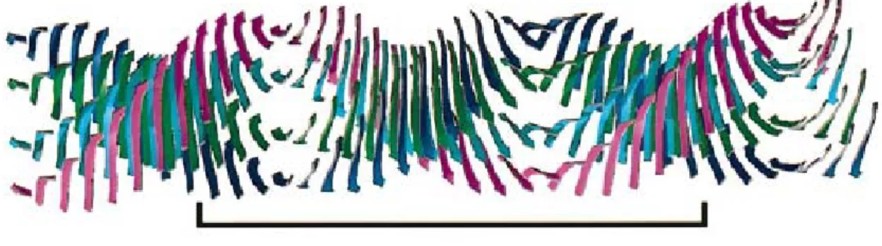
A number of studies were aimed at obtaining an insight into the macromolecular structure of amyloid fibrils using atomic force microscopy [Jansen et al. 2005; Khurana et al. 2003], electron microscopy [Jimenez et al., 2001, 2002] and even fluorescence microscopy [Ban et al., 2006]. Despite the diversity of amyloid-forming proteins, structural studies agree that all fibrils are composed of protofilaments – the smallest fibrillar subunits. Protofilaments can assemble into protofibrils and fibrils. Dimensions of protofilaments and their assemblies depend on the substrate protein (Fig. 2).

Although various models of fibril assembly from protofilaments can be supported by

microscopy images of selected specimen, overall mature fibrils are too different and too

inhomogenous to be described by a single model. Even the well-studied insulin amyloid

A B

C

Figure 2: Models of hierarchical assembly of protofilaments into amyloid fibrils. Protofilament pairs wind together to form protofibrils, and each two protofibrils wind to form a fibril in case of α-synuclein (A);

three protofilaments wind together to form a protofibril, and two protofibrils (or six protofilaments) wind

to form a fibril in case of the B1 domain of protein G (B), and protofilament pairs wind together to form

protofibrils, and each two protofibrils wind to form a type I fibril. Type II fibrils are the result of winding

of type I fibrils in the case of insulin (C) [adapted from Khurana et al. 2003].

still raises a lot of questions in developing a common definition of the mature fibril structure due to its polymorphism (Fig. 3).

Figure 3: Generalized scheme of the multipathway fibrillization of insulin. The lateral interaction of early, prefibrillar forms with protofibrils and protofilaments, followed by the lateral association of protofilaments, is a self-assembly route alternative to the hierarchical intertwining of protofilaments. The observed polymorphism of mature amyloid samples suggests that, under the given conditions, insulin fibrillization proceeds from both pathways [Jansen et al., 2005].

The internal structure of amyloid protofilaments was studied mainly by X-ray diffraction [Geddes et al., 1968; Sunde et al., 1997] and solid state NMR [Tycko 2000, 2003]. The x-ray diffraction patterns of amyloid fibrils reveal a periodic molecular structure consisting of polypeptide chains in the extended β-conformation, forming hydrogen-bonded-β-sheets which run parallel to the long axis of the fibril, whereas the constituent β-strands are arranged perpendicular to this axis. This data has led establishing the cross-β structure model of amyloid protofilaments (Fig. 4). Although other models, such as the β-helix [Raetz and Roderick, 1995; Lazo and Downing, 1998]

and predominantly native structures [Bouset et al., 2002; Inouye et al., 1998] were

described, the cross-β structure has a big support, including highly detailed structures for amyloid fibrils [Makin et al., 2005; Nelson et al., 2005].

115 Å, 24 β-strands

Figure 4: Molecular model of the common core protofilament structure of amyloid fibrils. A number of β- sheets (four illustrated here) make up the protofilament structure. These sheets run parallel to the axis of the protofilament, with their component β-strands perpendicular to the fibril axis. With normal twisting of the

protofilament, giving a helical repeat of 115.5 Å containing 24 β-strands (this repeat is indicated by the boxed region) [adapted from Sunde et al., 1997].

1.5. Mechanism of amyloid fibril formation

The most widely accepted and characterized mechanism of amyloid formation is the so-called “nucleation-elongation” or “nucleated growth” mechanism. Kinetic measurements of spontaneous aggregation usually show a lag phase, when no major changes are observed, followed by a rapid exponential growth phase [Nielsen et al., 2001; Serio et al., 2000]. The lag phase is defined as the time, required for the formation of “nuclei” – the structures which are able to grow into amyloid fibrils. Once the nucleus is formed, the fibril starts to grow by the attachment of either monomers or oligomers to the nucleus.

A lot of effort directed toward studying the nucleation process and the identification and characterization of the structures forming prior to fibrils has been made during the last decade. It has been shown that globular proteins need at least partial unfolding to be able to aggregate and form amyloid fibrils [Dobson, 1999;

Uversky and Fink, 2004]. In some cases the presence of structured oligomers [Kayed et

Figure 5: A schematic representation of some of the many conformational states that can be adopted by polypeptide chains. The transition from β-structured aggregates to amyloid fibrils can occur by addition of either monomers or protofibrils (depending on the protein) to preformed β-aggregates. All of these different conformational states and their interconversions are carefully regulated in the biological environment, much as enzymes regulate all the chemistry in cells, by using machinery such as molecular chaperones, degradatory systems, and quality control processes. Many of the various states of proteins are utilized functionally by biology, including unfolded proteins and amyloid fibrils, but conformational diseases will occur when such regulatory systems fail, just as metabolic diseases occur when the regulation of chemical processes becomes impaired [Chiti and Dobson, 2006].

al., 2004; Quintas et al., 2001] or unstructured aggregates [Kishnan and Lindquist, 2005;

Modler et al., 2003] has been reported. Polypeptide chains can adopt different

conformational states and interconvert between them on a wide range of timescales. The network of equilibria, which link some of the most important of such states both inside and outside the cell, is schematically illustrated in figure 5 [Chiti and Dobson, 2006].

1.6. Seeding

A nucleated growth mechanism has been well studied in other contexts such as crystallization of molecules [Jarrett and Lansbury, 1993]. As in other processes dependent on a nucleation step, the addition of preformed fibrillar species to a protein sample under aggregation conditions causes shortening or complete elimination of the lag phase [Serio et al., 2000]. Such an effect is known as seeding. In the context of the nucleated growth model, the addition of preformed fibrillar species can be equated to addition of nuclei, so that the elongation process can start without the additional time (lag phase) required for the nuclei formation. In many cases, the formation of nuclei requires destabilization of protein; in the case of some familial forms of diseases it is the

A

B

Figure 6: Under native conditions, the proteins are not able to form fibrils (A), but once preformed

fibrillar species are added, elongation of fibrils occurs (B).

primary mechanism through which natural mutations mediate their pathogenicity [Canet

et al., 2002]; but when preformed fibrillar species are added to a sample, elongation of

fibrils can proceed even under conditions, which are normally not favorable for nuclei

formation [Dzwolak et al., 2004a]. The ability of preformed amyloid fibrils to seed

native proteins under native conditions (Fig. 6) opens a new page in the history of

infectious particles by creating prions.

2. Materials and Methods

2.1. Materials

2.1.1. Chemicals

Chemicals, used for the experiments presented in this work are described in the following table (Table 3). For all experiemnts deionized water with (> 18 MΩ cm) was used, being obtained with the aid of an ELGA PURELAB Classic polisher system (ELGA LabWater, Celle, Germany).

Table 3: Chemicals, used for the experiments.

Material Supplier

Insulin from bovine pancreas Poly-D-lysine, 27.2 kDa (PDL) Deuterium oxide, 99.9 atom % D (D

O) Deuterium chloride, 99 atom % D (DCl) Ethyl alcohol-d, 99.5 atom % D (EtOD) Sodium deuteroxide, 99.5 atom % D (NaOD) Hydrochloric acid (HCl)

Ethyl alcohol (EtOH) Sodium chloride (NaCl)

Sodium phosphate, monobasic (NaH

PO

) Sodium phosphate, dibasic (Na

HPO

) Sodium hydroxide (NaOH)

2,2,2-Trifluorethanol (TFE) Glycerol

Thioflavin T (ThT) Chloroform (CHCl

)

Islet amyloid polypeptide (IAPP)

Sigma-Aldrich, Steinheim, Germany Sigma-Aldrich, Steinheim, Germany Sigma-Aldrich, Steinheim, Germany Sigma-Aldrich, Steinheim, Germany Sigma-Aldrich, Steinheim, Germany Sigma-Aldrich, Steinheim, Germany Merck, Darmstadt, Germany Sigma-Aldrich, Steinheim, Germany Merck, Darmstadt, Germany Sigma-Aldrich, Steinheim, Germany Sigma-Aldrich, Steinheim, Germany Merck, Darmstadt, Germany Merck, Darmstadt, Germany Sigma-Aldrich, Steinheim, Germany Merck, Darmstadt, Germany Merck, Darmstadt, Germany

Calbiochem

, Merck, Darmstadt, Germany

2.1.2. Insulin

Insulin is a hormone produced by β cells in the pancreas. It has three important functions: it allows glucose to pass into cells, suppresses excess production of sugar in the liver and muscles and suppresses the breakdown of fat for energy.

Insulin is a rather small protein, with a molecular weight of 5740 Daltons. It is composed of two peptide chains, referred to as the A chain and B chain. The chains are linked together by two disulfide bonds, and an additional disulfide is formed within the A chain. In most species, the A chain consists of 21 amino acids and the B chain of 30 amino acids (Fig. 7).

B chain, Mw 3400Da FVNQHLC GSHLVEALYLV CGERGFFYTPKA │ │

A chain, Mw 2340Da GIVEQCCASVCSLYQLENYCN │_____│

Figure 7: Primary structure of bovine insulin.

Although the amino acid sequence of insulin varies among species, certain segments of the molecule are highly conserved, including the positions of the three disulfide bonds, both ends of the A chain and the C-terminal residues of the B chain.

The similar amino acid sequences of insulin lead to similar three dimensional conformations of protein from different species, and the insulin from one particular animal is very likely biologically active in other species, as well. Indeed, pig insulin has been widely used to treat human patients.

A B C

Figure 8: A molecular model of bovine insulin. Monomer (A), dimer (B) and hexamer (C), with the A

chain colored blue and the larger B chain green [from the Protein data bank (file name 2a3g), picture

created using Biodesigner software].

The secondary structure of insulin is predominantly α-helical. Insulin molecules have a tendency to form dimers in solution due to hydrogen-bonding between the C- termini of the B chains. Additionally, in the presence of zinc ions, insulin dimers associate into hexamers (Fig. 8).

The ability of insulin to form fibrils under certain conditions was reported in the middle of the last century [Waugh, 1946; Waugh et al., 1950]. After the discovery of prions, the interest in amyloid fibril formation increased and insulin became one of the most popular model protein for these studies. But despite these efforts, comprehensive mechanisms of insulin fibrillation are still lacking.

2.1.3. Polylysine

Polylysine is a synthetic polymer. There are two main reasons, for which polylysine is an excellent, probably even the simplest model for protein aggregation studies. It undergoes an α-helix-to-β-sheet transition, the hallmark of protein aggregation, and forms amyloid-like fibrils [Fuhrhop et al., 1987; Fändrich and Dobson, 2002; Dzwolak et al., 2004c]. The sequenceless character of the polypeptide permits exploring of the hypothesis that aggregation is as a common generic feature of proteins as polymers taking place when native protein tertiary contacts are overruled by main- chain interactions [Dobson, 2004].

2.1.4. Islet amyloid polypeptide (IAPP)

IAPP (also known as amylin) is a 37 amino acid residue peptide hormone

[Lorenzo and Yankner, 1994] that is co-synthesized and co-secreted with insulin by

pancreatic β-cells [Cooper et al., 1989]. Several functions have been associated with the

soluble form of this hormone [Cooper et al., 1989; Johnson et al., 1992], including the

control of hyperglycemia by restraining the rate at which dietary glucose enters the

bloodstream. For reasons that are still not fully understood, IAPP aggregates in the

extracellular matrix of the β-cells forming fibrillar amyloid deposits. These deposits are

present in approximately 95 % of type II diabetes mellitus patients and are strongly

associated with degeneration and loss of islet β-cells [Westermark and Wilander, 1978;

Hayden, 2002].

It has been proposed that the IAPP aggregation process has two distinct phases: a lateral growth of oligomers followed by longitudinal growth into mature fibrils [Kayed et al., 1999; Padrick and Miranker, 2001, 2002; Green et al., 2004], and it has been demonstrated that the initial stages of IAPP fibril formation are driven by the increase of solvent-exposure of hydrophobicity patches [Kayed et al., 1999]. However, the structural changes behind the fibrillization process are still poorly understood.

2.2. Methods

2.2.1. Atomic Force Microscopy (AFM)

All images were recorded on a MultiMode scanning probe microscope equipped with a Nanoscope IIIa Controller from Digital Instruments (Santa Barbara, California, USA). The microscope was coupled to an AS-12 E-scanner (13-µm) or J-scanner (100- µm) and an Extender Electronics Module EX-II (Santa Barbara, California, USA), which allows for acquisition of phase images. Typically used AFM-probes were aluminum-coated NCHR silicon SPM sensors (force constant = 42 N/m; length = 125 µm; resonance frequency ≈ 250-330 kHz; nominal tip radius of curvature ≤ 5 nm) from Nanosensors, Nanoworld or Budgetsensors. The AFM head with optical block and base was placed atop a commercially available active, piezo-actuated vibration-damping desk from Halcyonics (Göttingen, Germany). All measurements were done in the air using TappingMode™.

TappingMode™ (Fig. 9) AFM operates by scanning a tip attached to the end of an

oscillating cantilever across the sample surface. The cantilever is oscillated at or near its

resonance frequency with amplitude ranging typically from 20 nm to 100 nm. The tip

lightly “taps” on the sample surface during scanning, contacting the surface at the

bottom of its swing. The feedback loop maintains constant oscillation amplitude by

maintaining a constant root mean square of the oscillation signal acquired by the split

photodiode detector. The vertical position of the scanner at each (x,y) data point in

order to maintain a constant "setpoint" amplitude is stored by the computer to form the topographic image of the sample surface. By maintaining a constant oscillation amplitude, a constant tip-sample interaction is also preserved during imaging. The operation can take place in either ambient or liquid environment. When imaging in air, the typical amplitude of the oscillation allows the tip to contact the surface through the adsorbed fluid layer without getting stuck [Scanning probe microscopy training notebook, Digital Instruments].

Figure 9: Scheme of AFM measurements using the TappingMode™ [adapted from the scanning probe microscopy training notebook, Digital Instruments].

Samples were diluted with deionized water to a final concentration of 0.5-2 µM,

10-30 µl were applied onto freshly cleaved muscovite mica and allowed to dry.

2.2.2. Fourier-transform infrared spectroscopy (FTIR)

The FTIR spectra were recorded using the Nicolet MAGNA 550, Nicolet NEXUS and Nicolet 5700 spectrometers from Thermo Scientific (Waltham, Massachusetts, USA) equipped with a liquid nitrogen cooled mercury-cadmium-telluride (MCT) detector. For all measurements, CaF

transmission windows and 0.05 mm Teflon or Mylar spacers were used. The temperature in the cell was controlled through an external water-circuit.

For each spectrum, 256 interferograms of 2 cm

resolution were co added. The sample chamber was continuously purged with dry air. From the spectrum of each sample, a corresponding buffer spectrum was subtracted. All the spectra were baseline-corrected and normalized prior to further data processing. The plots of the progress of α-helix–to–

β-sheet refolding upon aggregation were calculated as (I − I

)/(I

− I

), where I

is spectral intensity at 1625 cm

(or 1622 cm

in EtOD) of the native insulin (corresponding to the first spectrum), I

is the intensity after complete aggregation, and I is a transient intensity at this wavenumber. All data processing was performed with the GRAMS software (Thermo Scientific).

2.2.3. Ultrasonic resonator technology (URT)

The ultrasonic measurements were carried out using an ultrasonic resonator device (ResoScan system, TF Instruments GmbH, Heidelberg) with ultrasonic transducers made of single-crystal lithium niobate of a fundamental frequency of 9.5 MHz. The instrument comprises two independent cells for sample and reference with a path length of 7.0 mm. They are embedded into a metal block Peltier thermostat with a temperature stability of 0.001 °C. The resolution of the ultrasonic velocity measurements is 0.001 m s

. Ultrasonic velocities of the sample (U) and reference solvent (U

) were measured over the same temperature range and at the same heating rate.

The fundamental pre-condition for the propagation of acoustical waves in media is

the elastic coupling of the molecules to the media. For example, in solid phase materials

the atomic bodies are thought to be coupled via “spring-like bonds”, while in liquids

and gases elastic collisions are conceptualized as coupling intervals. In the absence of

sound, all these building elements are equally spaced, so that the mean force on them vanishes. Once this system is disturbed by a sudden and stepwise move of a rigid wall, the building blocks next to this wall get compressed and due to the described coupling, this compression propagates with the speed of sound (Fig. 10).

position x

pre s s u re

vibrating wall

compressed

expanded

direction of displacements

Figure 10: A periodically vibrating wall generates a wave field (black lines) were the displacements ξ of the building blocks results in areas of compressed and expanded density [Principles of sound measurement, TF Instruments].

If the wall moves periodically at the position x=0, a uniform wave field is created,

which means that at a fixed position x the same phase of motion is reached after the

time period T. The reciprocal of the time period T is the frequency f, usually expressed

in Hz. At a snapshot at a fixed time t the wave field has the same phase of motion at

points separated by the wavelength λ (along the direction of propagation). The wave is

mathematically described by a function ξ (x, t), which is the displacement of building

blocks from the rest position at position x and time t. Wavelength λ and frequency f

appear in this function as free parameters. Given the time period, T, for a propagation of

a length, λ , the speed of sound can be found:

U= λ /T= λ f (1) U is a constant for any material, which depends on the coupling strength between the building blocks of the medium.

The ResoScan system uses an acoustic resonator arrangement to measure the velocity of sound. The resonator consists of an ultrasonic sender and an ultrasonic receiver with the space between sender and transmitter filled with the sample fluid. A prerequisite for the high accuracy of measurements is the precise parallel alignment of sender and transmitter. Due to the reflection of sound at the transducers, a standing wave pattern can be established (Fig. 11A), but this is possible only at the ultrasonic wavelength λ

, were the distance D between sender and receiver is (n is dependent on the standing wave pattern (Fig. 11B)):

2 λ

n

D = (2)

Generator Reflector Wave Reflection Standing Wave

Continuous supply of energy maintains standing wave Transducer of LiNbO₃coated with gold

D

Transduc er Transducer

λ λ/2

A

B

Generator Reflector

Generator Reflector Wave ReflectionWave Reflection Standing WaveStanding Wave Continuous supply of energy maintains standing wave Transducer of LiNbO₃coated with gold

D

Transduc er Transducer

λ A

B

λ/2

Figure 11: Establishing standing wave between transducers (A) and standing wave pattern for n=1, 2, 3

and 73 (B) [adapted from Short training course, TF Instruments].

On the other hand, the wavelength λ is linked to the frequency f, and the velocity of sound in liquid U

, which is a characteristic for each wave transporting medium (here the fluid) via relation (1).

Since inside the resonator only standing waves with length λ

are allowed, only discrete frequencies f

may exist:

U

f

λ

= (3)

These frequencies f

are the real quantities to be measured by the Resoscan. This is done due to the fact that mostly the frequencies can be measured with high accuracy, while the length D of the resonator is held fixed and measured only once by the manufacturer.

The combination of (2) and (3) yields the frequencies at which standing waves inside the resonator may exist:

D n U f

2

=

(4)

In the terminology of ultrasonic interferometry, n is called the “peakorder”. For example for our Resonator of D=7 mm, U

=1498 m/s, one gets from (5) f

= n·107 kHz, which means the first resonance is at 107 kHz, the second at 214kHz, the 78th at 8.346 MHz, etc. (Fig. 12). The spacing between resonances is called the base frequency f

for the liquid:

D f U f

f

2

1 L

L

=

− = (5)

The above-mentioned approach implies the determination of the velocity of sound by measuring the difference between adjacent resonances f

, as well as the length D of the resonator, followed by using (5) to calculate the velocity.

However, under real experimental conditions, the measured sequence of

frequencies does not have exactly the same spacing (5) (due to the influence of the

natural frequency of the transducers, which is in the same range as the measured

frequencies of the fluid resonances). Since it is not obvious which of the several

spacings is to be considered for the determination of the velocity, this results in a large

error of the velocity determination.

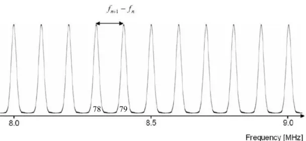
78 79

78 79

Figure 12: Schematic view of resonances in an ideal resonator with the dimensions of the ResoScan®

System in the range from 8 to 9 MHz. Sample: water at 25.4 °C, U = 1498 m/s, D = 7.0 mm [Introduction into the Ultrasonic Resonator Technology, TF Instruments].

A theoretical model of the resonator shows that, in the vicinity of the “natural frequency” of the ultrasonic transducers f

, significant deviations from the equal spaced model (4) exist. These deviations “y

” of the measured frequencies from the harmonic row (4) can be described by a simulation function y

:

⎟ ⎟

⎟ ⎟

⎟

⎠

⎞

⎜ ⎜

⎜ ⎜

⎜

⎝

⎛

⎟⎟ ⎠

⎜⎜ ⎞

⎝ + ⎛

−

−

=

R R

R L k L

π tan arctan π ) 2 Θ(

2 2

f z f

f z f D n

y U

n

n

(6)

with

⎩ ⎨

⎧

>

= <

−

R R R

1 for

for ) 0

Θ( f f

f f f

f

n n n

where z

is acoustical impedance of the fluid, z

is acoustical impedance of the transducers, f

is natural frequency of the transducers and f

is measured frequency of order n.

Fitting the simulation function (6) to the measured deviations of the observed resonances to the harmonic row delivers the parameters of the function.

This method is used at the initial setup (at the manufacturer) of a new resonator, to determine for a fluid of known U

and z

, the following resonator-specific values: D, z

and f

. These parameters are fixed in the operating software.

Conversely, U

and z

of the investigated fluid can be determined with the already known parameters D, z

and f

of the resonator. This is done automatically during the initialization process of the operating software.

After the initialization process of the device, the velocity of sound in the fluid as well as the correction for every resonator mode is known. Therefore it is appropriate to measure a single Resonator mode repeatedly with high accuracy, to follow the velocity of sound in the sample with respect to time or temperature. The single repeatedly measured mode is called the “Master Peak”.

The measurement of this single Master Peak is done in a so-called “phase scanning mode”, were the resonator mode is sampled with very high accuracy. From the amplitude vs. frequency curve, a polynomial fit is done by the operation software to get the best value for the velocity of the sample [Principles of sound measurement, TF Instruments].

2.2.4. Densitometry

Density measurements were carried out with a DMA 58 density meter from Anton Paar (Graz, Austria) with a precision of ±5·10

g/cm

, or DMA 5000 from Anton Paar GmbH (Graz, Austria) with a precision of ±5·10

g/cm

.

Both density meters determine the density ρ of liquids and gasses by measuring

the period of oscillation. To this end, the sample is introduced into a system which can

oscillate and whose “natural frequency” is influenced by the mass of the sample. This

system is a U-shaped tube which is excited to undamped oscillations by electronic

means. Both straight sections of the U-shaped tube form the spring element of the

oscillator. The direction of the oscillation is perpendicular to the plane of the U-shaped

tube. The oscillating volume V is limited by the mounting points which are fixed. If the

oscillator has been filled with the sample at least up to the mounting points, then the

same known volume V of the sample also oscillates. The mass of the sample can

therefore be considered as proportional to its density. If the oscillator has been filled

beyond the mounting points, this has no effect on the measurement. For this reason, the

oscillator can also measure the densities of samples flowing through it.

Assuming that the temperature is held constant, the density can be calculated from the period by considering a hollow body with mass M suspended on a spring constant s.

The volume V of the hollow body is then filled with a sample of density ρ. The natural frequency of this spring mass system is:

V M

s f π

ρ

= + 2

1 (7)

and the period T is:

s V

T = 2 π M ⁺ ρ (8)

Density dependent on the period T is:

V M V s

T −

=

4 π

ρ (9)

Using the abbreviations A=c/4π

V and B=M/V, we arrive at B

AT −

=

ρ (10)

The constants A and B comprise the spring constant of the oscillator, the mass of the empty tube and the volume of the sample involved in the oscillation. A and B are therefore device constants for each individual oscillator. They can be derived from two period measurements when the oscillator has been filled with substances of known density [User manual, Anton Paar].

The partial specific volume of the protein has been calculated using c

c c

v

= 1 / − ( ρ − ) / ρ

(11)

ρ and ρ

are the densities of the solution and solvent, respectively; c is the specific concentration of the protein.

2.2.5. Differential scanning calorimtery (DSC) and Pressure perturbation calorimetry (PPC)

DSC and PPC measurements were carried out on a VP DSC calorimeter from

MicroCal (Northampton, MA) equipped with the MicroCal’s PPC accessory. For the

DSC measurements, both cells of the calorimeter were first filled with buffer and a scan

was performed. Immediately after the scan, the buffer was removed from the sample

cell, replaced with ca. 0.5 mL sample and the measurement was performed. Buffer-

buffer data were subtracted from sample-buffer data. The specific heat capacity of the protein at constant pressure has been obtained from

0o 0 o ,

/ /

∆ C m v c v

c

=

+

(12)

C

∆ is the heat capacity difference between the sample solution and solvent reference cell as obtained by a the measurement; and are the partial specific volumes of the solute and solvent, respectively.

v

v

For the PPC measurements, gas (N

) pressure jump applied to the samples was 5 bars. Under the same experimental conditions, a set of reference sample-buffer, buffer- buffer, buffer-water, and water-water measurements was carried out each time. The values of partial specific volumes used for volumetric calculations were obtained from density measurements.

2.2.6. Fluorescence Spectroscopy

Fluorescence measurements were carried out on a K2 multifrequency phase and modulation fluorometer (ISS, Urbana, IL). The measurements were performed within a high-pressure cell (ISS), equipped with sapphire windows, and the pressure was controlled by an automated pressure control system (APP, Ithaca, NY).

Insulin and the fibril-specific dye Thioflavine T (ThT) were dissolved in H

O (pH 1.9) at a final protein to dye molar ratio of 50:1. The emission intensity at 482 nm was recorded upon excitation at 450 nm as a function of time t. The data were normalized by dividing the intensity at every point to the intensity recorded for the final aggregates.

2.2.7. Calculation of compressibilities

The most accurate method of determining the partial molar compressibility, , of a solute is based on the Newton-Laplace equation, which relates the coefficient of adiabatic compressibility of a medium,

So

K

( )( )

S

V V p

β = − 1 / ∂ / ∂ (13)

with its density, ρ , and sound velocity, U [Gekko and Hasegawa, 1986,1989; Taulier and Chalikian, 2002; Chalikian, 2003]:

(14)

1 2

= ( β

ρ )

U

For (infinitely) dilute solutions [Taulier and Chalikian, 2002; Chalikian, 2003],

(

)

o 0

S

β 2 V 2 [ U ] M / ρ

K =

− − (15)

where

S

V

K

=

β (16)

and

p

n

V

V

= ( ∂ / ∂ )

(17)

is the partial molar volume of the solute, M its molar mass, and

[U] = (U-U

)/(U

C) (18)

is the relative molar sound velocity (increment) of the solute; U and U

are the sound velocities of the solute and solvent, respectively.

Experimental data on

o o

/ V K

T

=

β (19)

of proteins are very scarce as it is technically challenging to measure the partial specific volume as a function of the pressure using densimetric techniques with high precision [Seemann et al. 2001]. However, the partial molar isothermal compressibility of the solute can be obtained from the adiabatic value by [Taulier and Chalikian, 2002;

Chalikian, 2003]

( ^{/( )} )( ^{2 /}

^/(

⁾ )

o 0 0 2 0

o 0

o S p p p

T

K T c E C c

K = + α ρ α − ρ (20)

where c

is the specific heat capacity at constant pressure of the solvent, α

is the coefficient of thermal expansion of the solvent, respectively, and

(21)

T

V

E

= ( ∂

/ ∂ )

is the partial molar expansibility of the solute, which can be determined with high precision from pressure perturbation calorimetric measurements [Ravindra and Winter, 2003; Schreiner et al., 2004]. is the partial molar heat capacity of the solute, and T is the absolute temperature.

op

C

3. Results and discussion

3.1. Insulin aggregation and amyloidogenesis

3.1.1. Effect of co-solvents

A 2% solution of insulin in D

O with 0.1 M NaCl (with or without 20% ethanol, TFE or glycerol), pD-adjusted to 1.9 was used (pH-meter readout +0.4 [Makhatadze et al., 1995]). The temperature was increased continuously at a rate of 20 ºC/h.

1700 1650 1600 1550 1500 1450

Wavenumber

A

Amide I/I’ band

Amide II band Amide II’ band

1700 1650 1600 1550 1500 1450

Wavenumber / cm

A

Amide I/I’ band

Amide II band Amide II’ band

1700 1650 1600 1550 1500 1450

Wavenumber

A

Amide I/I’ band

Amide II band Amide II’ band

1700 1650 1600 1550 1500 1450

Wavenumber / cm

A

Amide I/I’ band

Amide II band Amide II’ band

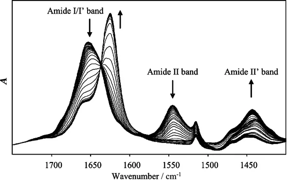
Figure 13: Time resolved FTIR spectra of insulin during heating and incubation at 60 ºC

With the increase of temperature, the amide II band (1543 cm

) decreases and

amide II’ (1445 cm

) increases because of H-D exchange (Fig. 13). Monitoring this

process allows one to follow the exposure of the protein to the solvent, which is related

to partial unfolding (Fig. 14). Experiments show that full H-D exchange in 20% ethanol

is completed just below 45ºC, in 20% glycerol and in pure D

O at around 47ºC, and in

20% TFE at about 50ºC. Ethanol seems to destabilize native α-helical structures of

insulin, TFE stabilizes them and glycerol seems to have no significant effect at this stage.

R el ati ve ar ea of a m id e -I I band R el ati ve ar ea of a m id e -I I band

20% Ethanol 20% TFE 20% Glycerol D₂O

D₂O

0 10 20 30 40 50 60

0,00 0,02 0,04 0,06 0,08 0,10 0,12

R el ati ve ar ea of a m id e -I I band R el ati ve ar ea of a m id e -I I band R el ati ve ar ea of a m id e -I I band R el ati ve ar ea of a m id e -I I band / a.u.

Temperature / °C

20% Ethanol 20% TFE 20% Glycerol D₂O

D₂O D₂O D₂O

0 10 20 30 40 50 60

0,00 0,02 0,04 0,06 0,08 0,10 0,12

0 10 20 30 40 50 60

0,00 0,02 0,04 0,06 0,08 0,10 0,12

0 10 20 30 40 50 60

0,00 0,02 0,04 0,06 0,08 0,10 0,12

R el ati ve ar ea of a m id e -I I band R el ati ve ar ea of a m id e -I I band R el ati ve ar ea of a m id e -I I band R el ati ve ar ea of a m id e -I I band

20% Ethanol 20% TFE 20% Glycerol D₂O

D₂O D₂O D₂O

0 10 20 30 40 50 60

0,00 0,02 0,04 0,06 0,08 0,10 0,12

0 10 20 30 40 50 60

0,00 0,02 0,04 0,06 0,08 0,10 0,12

0 10 20 30 40 50 60

0,00 0,02 0,04 0,06 0,08 0,10 0,12

R el ati ve ar ea of a m id e -I I band R el ati ve ar ea of a m id e -I I band R el ati ve ar ea of a m id e -I I band R el ati ve ar ea of a m id e -I I band / a.u.

Temperature / °C

20% Ethanol 20% TFE 20% Glycerol D₂O

D₂O D₂O D₂O

0 10 20 30 40 50 60

0,00 0,02 0,04 0,06 0,08 0,10 0,12

0 10 20 30 40 50 60

0,00 0,02 0,04 0,06 0,08 0,10 0,12

0 10 20 30 40 50 60

0,00 0,02 0,04 0,06 0,08 0,10 0,12

0 10 20 30 40 50 60

0,00 0,02 0,04 0,06 0,08 0,10 0,12

Figure 14: H-D exchange rate monitored in the presence of different co-solvents.

A further increase in temperature and further incubation at 60 ºC leads to changes of the secondary structure, from α-helix to β-sheet, which is reflected in the decrease of the peak around 1650 cm

and the increase of the peak in the region between 1620- 1630 cm

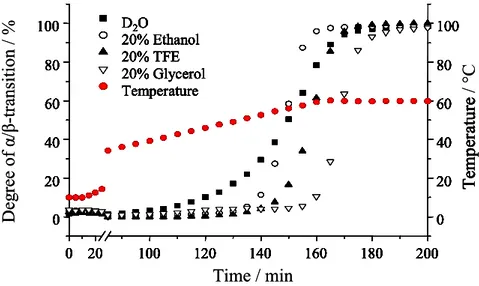
of the amide I/I’ band (Fig. 13). The kinetics of aggregation under different conditions was monitored by plotting the relative extent of α/β-transition (Fig. 15). The presence of glycerol or TFE seems to stabilize α-helical structures, while the aggregation curve in the presence of ethanol shows similar a midpoint when compared with the one in pure D

O. The main difference is the faster rate of aggregation.

Tem per at ur e

0 20 100 120 140 160 180 200

0 20 40 60 80 100

0 20 40 60 80 D₂O 100

20% Ethanol 20% TFE 20% Glycerol Temperature

Tem per at ur e

0 20 100 120 140 160 180 200

0 20 40 60 80 100

0 20 40 60 80 D₂O 100

20% Ethanol 20% TFE 20% Glycerol Temperature

Tem per at ur e / °C

De gr ee of α / β -t ra nsition / %

0 20 100 120 140 160 180 200

0 20 40 60 80 100

0 20 40 60 80 D₂O 100

20% Ethanol 20% TFE 20% Glycerol Temperature

0 20 100 120 140 160 180 200

0 20 40 60 80 100

0 20 40 60 80 100

0 20 100 120 140 160 180 200

0 20 40 60 80 100

0 20 40 60 80 D₂O 100

20% Ethanol 20% TFE 20% Glycerol Temperature

Time / min

Tem per at ur e

0 20 100 120 140 160 180 200

0 20 40 60 80 100

0 20 40 60 80 D₂O 100

20% Ethanol 20% TFE 20% Glycerol Temperature

Tem per at ur e

0 20 100 120 140 160 180 200

0 20 40 60 80 100

0 20 40 60 80 100

0 20 100 120 140 160 180 200

0 20 40 60 80 100

0 20 40 60 80 D₂O 100

20% Ethanol 20% TFE 20% Glycerol Temperature

Tem per at ur e

0 20 100 120 140 160 180 200

0 20 40 60 80 100

0 20 40 60 80 D₂O 100

20% Ethanol 20% TFE 20% Glycerol Temperature

0 20 100 120 140 160 180 200

0 20 40 60 80 100

0 20 40 60 80 100

0 20 100 120 140 160 180 200

0 20 40 60 80 100

0 20 40 60 80 D₂O 100

20% Ethanol 20% TFE 20% Glycerol Temperature

Tem per at ur e / °C

De gr ee of α / β -t ra nsition / %

0 20 100 120 140 160 180 200

0 20 40 60 80 100

0 20 40 60 80 100

0 20 100 120 140 160 180 200

0 20 40 60 80 100

0 20 40 60 80 D₂O 100

20% Ethanol 20% TFE 20% Glycerol Temperature

0 20 100 120 140 160 180 200

0 20 40 60 80 100

0 20 40 60 80 100

0 20 100 120 140 160 180 200

0 20 40 60 80 100

0 20 40 60 80 D₂O 100

20% Ethanol 20% TFE 20% Glycerol Temperature

Time / min

Figure 15: Aggregation kinetics of insulin monitored in the presence of different co-solvents

The final spectral positions of the amide I’ band depend on the presence of co- solvents during the aggregation process (Fig 16). Amide I’ band positions are as follows:

in case of 20% TFE – 1621 cm

, 20% ethanol – 1622 cm

, pure D

O – 1625 cm

, and 20% glycerol – 1626 cm

. A red shift of the band suggests stronger interstrand hydrogen bonds in the aggregates formed in the presence of ethanol and TFE, while the small blue shift suggests weaker interstrand hydrogen bonds in the aggregates formed in the presence of glycerol. Similar observations have been reported previously for insulin amyloids grown in the presence of ethanol [Dzwolak et al., 2004] and acetic acid [Nielsen et al., 2004]. Taken together, the data suggests the ability of insulin to form different final amyloid structures starting from the same amino acid sequence.

1700 1680 1660 1640 1620 1600 1580 1700 1680 1660 1640 1620 1600

Glycerol, 1626 cm

D

O, 1625 cm

TFE, 1621 cm

Ethanol, 1622 cm

A

1700 1680 1660 1640 1620 1600 1580 1700 1680 1660 1640 1620 1600

Glycerol, 1626 cm

D

O, 1625 cm

TFE, 1621 cm

Ethanol, 1622 cm

Wavenumber / cm

A

1700 1680 1660 1640 1620 1600 1580 1700 1680 1660 1640 1620 1600

Glycerol, 1626 cm

D

O, 1625 cm

TFE, 1621 cm

Ethanol, 1622 cm

A

1700 1680 1660 1640 1620 1600 1580 1700 1680 1660 1640 1620 1600

Glycerol, 1626 cm

D

O, 1625 cm

TFE, 1621 cm

Ethanol, 1622 cm

Wavenumber / cm

A

Figure 16: Amide I’ band of final insulin amyloid aggregates in different co-solvents.

3.1.2. Sonication of amyloid fibrils

0.5 % insulin was dissolved in HCl, pH 2, and incubated for 40 hours at 60°C to

induce formation of fibers (Fig. 17A). The sample was subjected to an ultrasonic bath

(45 kHz, 30W) for different times. This leads to braking of fibers into shorter pieces

(Figs. 17B and C).

A B C

E F

D

Figure 17: AFM pictures of insulin amyloid fibrils. Before sonication (A); after 30 min sonication (B); 3 hours sonication (C); 24 hours (D), 72 hours (E) and 168 hours (F) incubation at room temperature.

Sonicated fibers were kept at room temperature for a week to check if broken pieces could reconnect together. The process of fibrils sticking together is rather slow – there were no long fibrils found after 24 hours of incubation (Fig. 17D). Though further incubation leads to formation of colonies, including fibril-like particles (Fig. 17E) of a similar length as the fibrils have before sonication (Fig. 17A). A closer look at the AFM pictures shows that most of the broken fibrils stick together via their ends (Fig. 17F), suggesting that broken fibrils are probably more prone to attach additional particles and thus elongate.

3.1.3. Seed induced aggregation

The seed-induced aggregation of bovine insulin at pD 1.9 and 25°C was followed

by time-resolved FTIR spectroscopy (Fig. 18A). The infrared spectra show a gradual

shift of the amide I’ band to 1625 (in acidified D

O) or 1622 (acidified 20% (v/v)

ethanol in D

O) cm

, accompanied by a marked narrowing of the peak, both of which reflect the complete transition of the native structure into nonnative aggregated β- strands. The amyloidal character of the final insulin aggregates was confirmed by atomic force microscopy scans, which exhibit typical fibrils (Fig. 18B).

1543 cm^-1

1750 1700 1650 1600 1550 1500 1450 1400 1750 1700 1650 1600 1550 1500 1450 1400

Native insulin Aggregated

1543 cm^-1

A

A B

1543 cm^-1

1750 1700 1650 1600 1550 1500 1450 1400 1750 1700 1650 1600 1550 1500 1450 1400

Native insulin

β-sheet

1543 cm^-1

A

Wawenumber / cm

A B

1543 cm^-1

1750 1700 1650 1600 1550 1500 1450 1400 1750 1700 1650 1600 1550 1500 1450 1400

Native insulin Aggregated

1543 cm^-1

A

A B

1543 cm^-1

1750 1700 1650 1600 1550 1500 1450 1400 1750 1700 1650 1600 1550 1500 1450 1400

Native insulin

β-sheet

1543 cm^-1

A

Wawenumber / cm

A B

Figure18: Seeds-induced aggregation of insulin. (A) Time-dependent changes in FT-IR spectra show the gradual evolution of the amide I’ band of insulin reflecting the structural transition from the native form to amyloid: 2% (w/w) bovine insulin in 0.1 M NaCl in D

O, pD1.9, seeded at 25°C at a 20:1 weight ratio with preformed seeds. The total elapsed time between the first and the final spectrum was 20 h. Arrows show directions of the spectral changes. (B) A height-scan AFM image of the final insulin aggregate.

The position of the amide I’ band at 1622 or 1625 cm

is the fundamental spectral difference between insulin amyloids grown spontaneously (unseeded) at 60°C in the presence or absence of 20% (v/v) d

-deuterated ethanol (EtOD), respectively (Fig.

19A). Although in either case, the band’s shapes and positions are characteristic for the

amyloid’s parallel β-sheet structure, it is red-shifted for EtOD-grown samples (1622

versus 1625 cm

for D

O-grown amyloid (Fig. 19A)). According to corresponding

second derivative spectra (Fig. 19B), this shift should be specifically attributed to an

increasing β-sheet fraction at 1620 cm

. The mature amyloid fibrils do not exhibit any

spectral changes after being resuspended in an alternative solvent (data not shown).