Iris Recognition

Machine Learning Techniques and Optical Systems for

Iris Recognition

from Distant Viewpoints

Dissertation

zur Erlangung des Doktorgrades der Naturwissenschaften (Dr. rer. nat.)

der Fakultät Physik der Universität Regensburg

vorgelegt von Florian S. Langgartner

aus Regensburg

im Jahr 2019

Die vorliegende Dissertation entstand während einer dreijährigen Zusammenar- beit mit der Firma Continental Automotive GmbH, ansässig in der Siemens- straße 12 in 93055 Regensburg.

Das Promotionsgesuch wurde am 14.05.2019 eingereicht.

Die Arbeit wurde von Prof. Dr. Elmar Lang angeleitet.

Prüfungsausschuss:

Vorsitzender: Prof. Dr. Josef Zweck 1. Gutachter: Prof. Dr. Elmar Lang 2. Gutachter: Dr. Stefan Solbrig

weiterer Prüfer: PD Dr. Alfred Weymouth

Contents

1 Introduction 1

2 Techniques 5

2.1 Histogram Equalization . . . . 6

2.2 CLAHE . . . . 7

2.3 Z-Score Transform . . . . 7

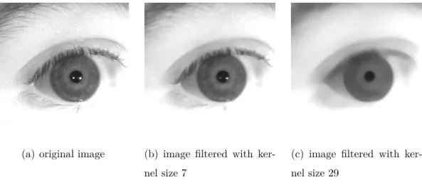
2.4 Sharpening Filters . . . . 8

2.5 Median Filtering . . . . 10

2.6 Hough Transform . . . . 11

2.6.1 Canny Edge Detection . . . . 11

2.6.2 Hough Line Transform . . . . 12

2.6.3 Hough Circle Transform . . . . 13

3 Optical Systems 15 3.1 Foscam IR Night Vision Camera . . . . 16

3.1.1 Camera . . . . 16

3.1.2 Pictures . . . . 17

3.2 Basler Automotive Camera . . . . 19

3.2.1 Camera, Sensor, Objective Lens and NIR LEDs . . . . . 19

3.2.2 Pictures . . . . 22

3.3 Auto Focus . . . . 24

4 Database 29

5 Iris Recognition 33

5.1 Preprocessing . . . . 36

5.1.1 Sharpness Check . . . . 36

5.1.2 Brightness Invariance . . . . 39

5.1.3 Eye Gaze Removal . . . . 41

5.2 Segmentation . . . . 43

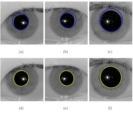
5.2.1 Hough Circle Transform . . . . 44

5.2.2 Snake Algorithm . . . . 46

5.2.3 Segmentation in the Polar Representation . . . . 51

5.2.4 Unet Segmentation . . . . 53

5.2.5 Performance . . . . 56

5.3 Noise Removal . . . . 59

5.3.1 Hough Transform . . . . 60

5.3.2 Variance Based Removal . . . . 61

5.3.3 Canny Based Removal . . . . 62

5.3.4 Adaptive Thresholding . . . . 63

5.3.5 Performance . . . . 65

5.4 Segmentation Quality Check . . . . 68

5.4.1 Shape Count Check . . . . 69

5.4.2 Histogram Based Check . . . . 70

5.4.3 Performance . . . . 72

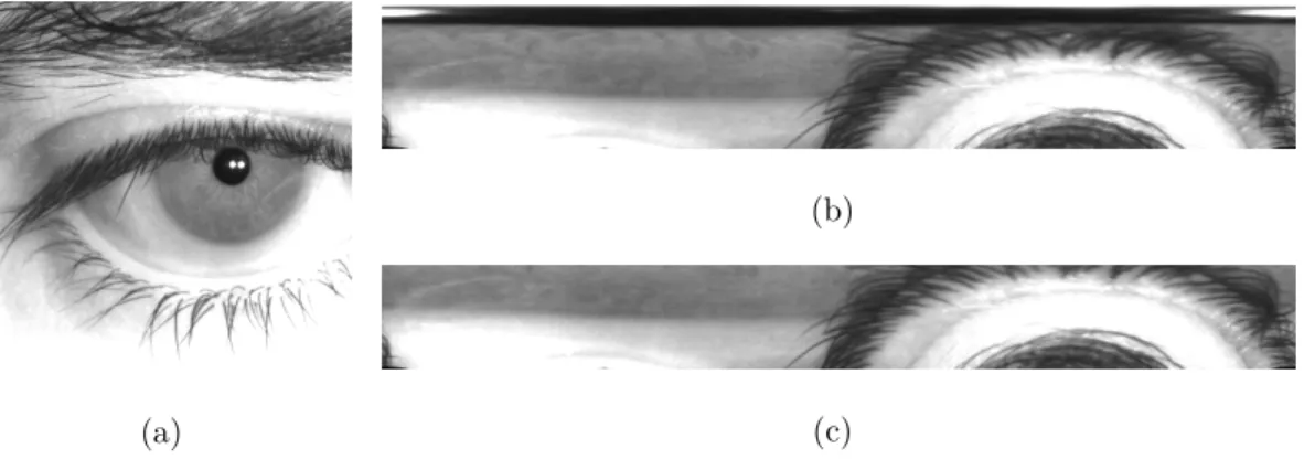
5.5 Normalization . . . . 74

5.6 Feature Extraction . . . . 78

5.6.1 1D Log-Gabor Filter . . . . 79

5.6.2 2D-Gabor Filter . . . . 79

5.6.3 Phase Quantization . . . . 80

5.6.4 Performance . . . . 82

5.7 Matching . . . . 83

5.7.1 Hamming Distance . . . . 83

5.7.2 Rotational Invariance . . . . 84

5.7.3 Score Normalization . . . . 86

5.7.4 Template Weighting . . . . 87

vi

5.7.5 Performance . . . . 89

6 Periocular Recognition 93 6.1 Feature Extraction . . . . 94

6.1.1 Local Binary Pattern Histogram (LBPH) . . . . 95

6.1.2 Z-Images . . . . 97

6.1.3 Deep Neural Networks . . . . 99

6.1.3.1 Deep Belief Network . . . . 99

6.1.3.2 Residual Neural Network . . . 101

6.2 Classifiers . . . 103

6.2.1 Cosine Distance . . . 103

6.2.2 Jensen-Shannon Divergence . . . 104

6.3 Performance . . . 105 7 Liveness Detection and Anti-Spoofing 109

8 Performance 115

9 Conclusion and Prospects 123

A Images recorded with the FOSCAM Night Vision Camera 127

B Images recorded with the Basler Automotive Camera 129

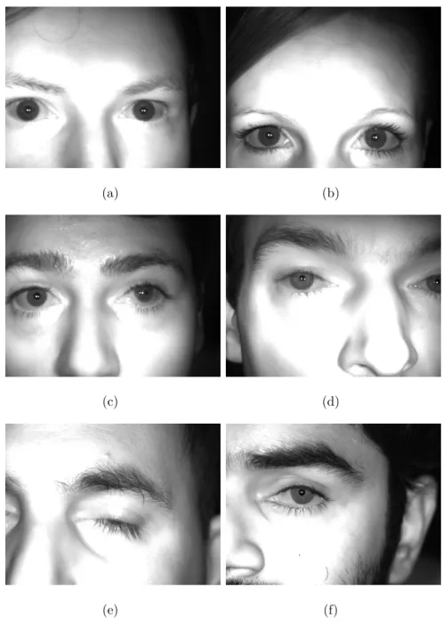
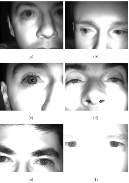
C Images from the Self-Recorded Database 133

Abstract

Vorhergehende Studien konnten zeigen, dass es im Prinzip möglich ist die Meth- ode der Iriserkennung als biometrisches Merkmal zur Identifikation von Fahrern zu nutzen. Die vorliegende Arbeit basiert auf den Resultaten von [35], welche ebenfalls als Ausgangspunkt dienten und teilweise wiederverwendet wurden.

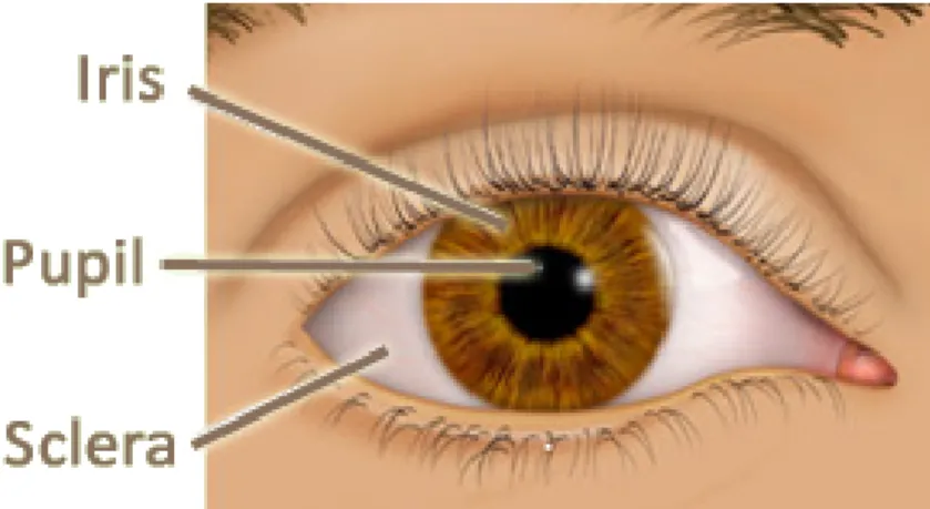
Das Ziel dieser Dissertation war es, die Iriserkennung in einem automotiven Umfeld zu etablieren. Das einzigartige Muster der Iris, welches sich im Laufe der Zeit nicht verändert, ist der Grund, warum die Methode der Iriserkennung eine der robustesten biometrischen Erkennungsmethoden darstellt.

Um eine Datenbasis für die Leistungsfähigkeit der entwickelten Lösung zu schaffen, wurde eine automotive Kamera benutzt, die mit passenden NIR-LEDs vervollständigt wurde, weil Iriserkennung am Besten im nahinfraroten Bereich (NIR) durchgeführt wird.

Da es nicht immer möglich ist, die aufgenommenen Bilder direkt weiter zu ve- rabeiten, werden zu Beginn einige Techniken zur Vorverarbeitung diskutiert.

Diese verfolgen sowohl das Ziel die Qualität der Bilder zu erhöhen, als auch

sicher zu stellen, dass lediglich Bilder mit einer akzeptablen Qualität verar-

beitet werden. Um die Iris zu segmentieren wurden drei verschiedene Algo-

rithmen implementiert. Dabei wurde auch eine neu entwickelte Methode zur

Segmentierung in der polaren Repräsentierung eingeführt. Zusätzlich können

die drei Techniken von einem "Snake Algorithmus", einer aktiven Kontur Meth-

ode, unterstützt werden. Für die Entfernung der Augenlider und Wimpern aus dem segmentierten Bereich werden vier Ansätze präsentiert. Um abzusichern, dass keine Segmentierungsfehler unerkannt bleiben, sind zwei Optionen eines Segmentierungsqualitätschecks angegeben. Nach der Normalisierung mittels

"Rubber Sheet Model" werden die Merkmale der Iris extrahiert. Zu diesem Zweck werden die Ergebnisse zweier Gabor Filter verglichen. Der Schlüssel zu erfolgreicher Iriserkennung ist ein Test der statistischen Unabhängigkeit.

Dabei dient die Hamming Distanz als Maß für die Unterschiedlichkeit zwischen der Phaseninformation zweier Muster. Die besten Resultate für die benutzte Datenbasis werden erreicht, indem die Bilder zunächst einer Schärfeprüfung unterzogen werden, bevor die Iris mittels der neu eingeführten Segmentierung in der polaren Repräsentierung lokalisiert wird und die Merkmale mit einem 2D-Gabor Filter extrahiert werden.

Die zweite biometrische Methode, die in dieser Arbeit betrachtet wird, benutzt die Merkmale im Bereich der die Iris umgibt (periokular) zur Identifikation.

Daher wurden mehrere Techniken für die Extraktion von Merkmalen und deren Klassifikation miteinander verglichen. Die Erkennungsleistung der Iriserken- nung und der periokularen Erkennung, sowie die Fusion der beiden Methoden werden mittels Quervergleichen der aufgenommenen Datenbank gemessen und übertreffen dabei deutlich die Ausgangswerte aus [35].

Da es immer nötig ist biometrische Systeme gegen Manipulation zu schützen, wird zum Abschluss eine Technik vorgestellt, die es erlaubt, Betrugsversuche mittels eines Ausdrucks zu erkennen.

Die Ergebnisse der vorliegenden Arbeit zeigen, dass es zukünftig möglich ist biometrische Merkmale anstelle von Autoschlüsseln einzusetzen. Auch wegen dieses großen Erfolges wurden die Ergebnisse bereits auf der Consumer Elec- tronics Show (CES) im Jahr 2018 in Las Vegas vorgestellt.

x

Abstract

Previous research has shown that it is principally possible to use iris recog- nition as a biometric technique for driver identification. This thesis is based upon the results of [35], which served as a starting point and was partly reused for this thesis. The goal of this dissertation is to make iris recognition avail- able in an Automotive Environment. Iris recognition is one of the most robust biometrics to identify a person, as the iris pattern is unique and does not alter its appearance during aging.

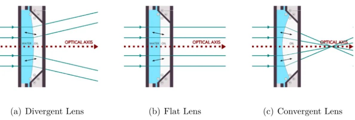
In order to create the database, which was used for the performance evalua- tions in this thesis, an Automotive Camera was utilized. As iris recognition is best executed in the near infrared (NIR) spectral range, due to the fact that even the darkest irises reveal a rich texture at these frequencies, the optical system is combined with suitable near infrared LEDs.

As the recorded images cannot always be processed right away, several prepro-

cessing techniques are discussed with the goal of enhancing the image quality

as well as processing only images that have an acceptable quality. In order

to segment the iris, three different algorithms were implemented. Thereby, a

newly developed Segmentation in the Polar Representation is introduced. In

addition, the three techniques can be enhanced by a Snake Algorithm, which is

an active contour approach. For removing the eyelids and eyelashes from the

segmented area, four noise removal approaches are presented. For the goal of

ensuring that no fatal segmentations slip through, two options for a segmen- tation quality check are given. After the normalization with the rubber sheet model, the feature extraction is responsible for collecting the iris information, therefore, the results using a 1D-Log Gabor Filter or a 2D-Gabor Filter are compared. In the end, the key to iris recognition is a test of statistical inde- pendence. For this reason, the Hamming Distance serves well as a measure of dissimilarity between the phase information of two patterns. The best results for the database in use are gained by checking the image with a Sharpness Check before segmenting the iris by utilizing the newly introduced Segmenta- tion in a Polar Representation and the 2D-Gabor Filter as feature extractor.

The second biometric technique that is considered in this thesis is periocular recognition. Thereby, the features in the area surrounding the iris are exploited for identification. Therefore, a variety of techniques for the feature extraction and the classification are compared to each other. The performances of iris recognition and periocular recognition as well as the fusion of the two biomet- rics are measured with cross comparisons of the recorded database and greatly exceed the initial values from [35].

Finally, it is always required to secure biometric systems against spoofing. In the course of this thesis a printout attack served as the scenario that should be prevented, wherefore a working countermeasure is presented.

The results of this thesis points to the possibility of utilizing biometrics as a personalized car key in the future. Due to this huge success, the findings were also presented at the Consumer Electronics Show (CES) in 2018 at Las Vegas, yielding a great amount of feedback.

xii

Chapter 1. Introduction

Chapter 1 Introduction

In the automotive industry four Megatrends can be identified. These are Safety, Environment, Affordable Cars and Information.

At first, the Safety Megatrend unites all those technologies that aim to increase the vehicle safety. The long term vision of automated driving, connected with the vision zero – zero fatalities, zero injuries, zero accidents – corresponds to this domain. It is currently most driven by Google and Tesla, the leaders con- cerning automated driving.

The Environment Megatrend tries to reach the goal of zero emissions, for exam- ple by using fewer fossil fuels. The carbon dioxide emissions shall be reduced in order to make the automotive world greener and cleaner, as well as less cli- mate harming. Recent developments especially in relation with, as well as due to, the exhaust gas scandal show intensified advances towards fully electrified vehicles and fuel cell engines.

The third Megatrend is to make the existing technologies available in Afford-

able Cars. Of course, prosperity gaps and diverse expectations on cars require

varying definitions for different parts of the world. In Western Europe and the

United States of America the price limit for affordable cars is about 10, 000 Eu-

Chapter 1. Introduction

ros, whereas people in other parts of the world could never afford this amount of money, nor would they label this as cheap.

Last but not least, the Information Megatrend deals with gathering and using more and more pieces of information. It aims at optimizing the selection of presented data in order to adequately inform the driver. Moreover, it is sup- posed to prevent overcharging the attention of the driver for allowing relaxed and secure driving.

This thesis aims to contribute to the progress in the Information Megatrend.

Since the possibility to robustly identify persons using biometric technology has been around for some years, the automotive industry wants to integrate these technologies in their environment, too. There are several possibilities to recognize individuals by biometric aspects, for example optically, thermally, capacitively or electrophorensicly. All of of them have different costs and se- curity levels.

Generally, the methods can be differentiated between static and dynamic. Dy- namic or behavioral biometric characteristics for example include gait analysis, voice analysis, signature analysis and keystroke dynamics. Common static or physiological biometric technology covers fingerprint recognition, face recogni- tion, DNA sequence analysis, retinal scans and many more.

One of the most secure methods with comparatively low costs and the benefit of a relatively low time consumption is iris recognition. It is ideal for an inte- gration in vehicles, as the required optical systems are already existing or will be available soon for modern cars.

This thesis is based upon the results of [35], which made the first steps towards iris recognition in an automotive environment from distant viewpoints, with realtime recognition and as little cooperation from the subjects as possible.

All this with the goal of enhancing theft protection by only allowing autho-

2

Chapter 1. Introduction

rized people to start the engine. Therefore, [35] served as a starting point and

was partially reused in this thesis. Similarly, the existing implementation using

Python and OpenCV [29] was reutilized as a base for the comprehensive ad-

vances that will be presented in the following chapters. On top of the presented

approaches, plenty other techniques were tried that will not be described, as

this would vastly increment the size of this thesis, though adding only little

additional information. The idea was to catch up with the open issues and

ideas of [35] and finally implement the system in a car demonstrator, always

keeping the long-term vision of completely replacing the car key by biometric

technology in mind, which requires excellent recognition rates.

Chapter 2. Techniques

Chapter 2 Techniques

The following chapter introduces some general computer vision and machine learning techniques that were used throughout this thesis. Histogram Equaliza- tion (see 2.1) is utilized to optimize the usage of the full range of allowed values in an image. Thereby, contrast is enhanced globally. Contrast Limited Adap- tive Histogram Equalization (CLAHE) (see 2.2) is an extension to Histogram Equalization. It enhances contrast not only globally but also locally. The Z- Score Transform (see 2.3) allows the standardization of distributions in a way that they become comparable to other distributions. In order to sharpen an image, two different Sharpening Filters (see 2.4) are presented, namely Lapla- cian Filters and a method named Unsharp Masking. Median Filtering (see 2.5) is a possibility to remove noise without smoothing the edges of an image.

Finally the Hough Transform (see 2.6) is a tool that can be used in order to

find simple geometric shapes, such as lines or circles. Thereby, usually a Canny

Edge Detector (see 2.6.1) is utilized, which is a commonly used technique for

edge detection, based on Sobel Filtering.

2.1 Histogram Equalization Chapter 2. Techniques

2.1 Histogram Equalization

Histogram Equalization [51, 62] is a technique for adjusting intensities in order to enhance the overall image contrast by stretching the intensity range. The distribution of a histogram is mapped to a more uniform and wide distribution of intensity values, making use of the maximum possible range. The first step for an 8 bit monochrome image with 256 possible intensities is to calculate the probability p(i), with which each intensity value occurs with. This is done by

p(i) = n

N , (2.1)

with n

as the number of pixels with intensity i ∈ [0, i

], i

= 255, and N the total number of pixels N . The cumulative distribution function F

is given by

F

(i) =

i

X

j=0

p(j) . (2.2)

It has to be multiplied with the size of the intensity range i

, in order to obtain the complete transformation function T (i) [35]

T (i) = i

i

X

j=0

n

N

. (2.3)

6

Chapter 2. Techniques 2.2 CLAHE

2.2 CLAHE

Contrast Limited Adaptive Histogram Equalization (CLAHE) [62] is a way to increase the contrast of an image. Adaptive Histogram Equalization (AHE) is an extension to the normal Histogram Equalization (see 2.1), which computes multiple histograms for different neighborhoods of the image. By equalizing the respective section’s histograms, the local contrast is enhanced and illumination effects are evenly distributed. As AHE tends to amplify noise in images too much, the contrast is limited by clipping histogram bins, if they exceed a given value, the clip limit. Subsequently, the clipped parts are redistributed equally among all bins. This is then called Contrast Limited AHE or CLAHE [50].

As the calculation of multiple histograms is computationally expensive, it is possible to reduce complexity by interpolation or by a sliding window approach [61].

2.3 Z-Score Transform

The Z-Score Transform [33, 62] is used to standardize distributions in order to being able to compare differently distributed random variables. The Z-Score Transform Z of a value x from a sample X is given by

Z (x) = x − X ¯

σ

(2.4)

with X ¯ being the sample’s mean value and σ

the sample’s standard deviation.

In image processing, the application of the Z-Score Transform results in an

increased invariance to different illuminations. Important thereby is that due

to the resulting distribution’s mean value of zero and standard deviation of one,

the values will not be integers and might as well be negative, preventing an

2.4 Sharpening Filters Chapter 2. Techniques

interpretation as image intensity. Therefore, these values need to be rescaled back to the original 8-bit image space by normalization to the range of [0, 255].

2.4 Sharpening Filters

In order to sharpen an image, Sharpening Filters [51, 62] can be applied. For creating such filters, the Laplacian Operator L(x, y) of an image I(x, y)

L(x, y) = ∂

I

∂x

+ ∂

I

∂y

(2.5)

can be utilized. As images are represented by discrete pixel intensities, it is required to use discrete convolution kernels, which are approximations of the second derivatives in the Laplacian Operator L(x, y). The two most commonly used Laplacian Filters are

L

=















0 −1 0

−1 4 −1

0 −1 0















and L

=















−1 −1 −1

−1 8 −1

−1 −1 −1















. (2.6)

Applying these filters results in the enhancement of discontinuities and edges of an image on a featureless background. For finally obtaining the filtered image, the resulting Laplacian image is added to the original image. It is also possible to design the filters in a way that they perform both steps at once, in order to simplify the computation:

L

=















0 −1 0

−1 5 −1

0 −1 0















and L

=















−1 −1 −1

−1 9 −1

−1 −1 −1















. (2.7)

8

Chapter 2. Techniques 2.4 Sharpening Filters

Another possibility to sharpen an image is given by a technique called Unsharp Masking. Thereby, the image is enhanced by

I

= I

+ a · (I

− I

) (2.8)

with a as a value that adjusts the enhancement potency. The blurred image I

is obtained by either averaging the original image or using a Gaussian Filter. An example for the resulting Unsharp Masking filters M

with a size of 9 × 9 is given by

M

= 1 81

























































−1 −1 −1 −1 −1 −1 −1 −1 −1

−1 −1 −1 −1 −1 −1 −1 −1 −1

−1 −1 −1 −1 −1 −1 −1 −1 −1

−1 −1 −1 −1 −1 −1 −1 −1 −1

−1 −1 −1 −1 161 −1 −1 −1 −1

−1 −1 −1 −1 −1 −1 −1 −1 −1

−1 −1 −1 −1 −1 −1 −1 −1 −1

−1 −1 −1 −1 −1 −1 −1 −1 −1

−1 −1 −1 −1 −1 −1 −1 −1 −1

























































. (2.9)

2.5 Median Filtering Chapter 2. Techniques

2.5 Median Filtering

In order to perform Median Filtering [51, 62], the median of the pixels in a defined neighborhood area is taken as the new pixel value. Thereby, noise is effectively removed, without smoothing the edges, which makes it a suitable tool for facilitating the segmentation (see 5.2) of images. Bigger kernels can even remove larger distortions, such as reflections. Figure 2.1 shows the impact of Median Filtering on an image from the self-recorded database (see chapter 4). The left image is the original. The other two pictures were filtered with kernel sizes of 7 for the middle one and 29 for the right one, respectively. In the slightly filtered image the smoothing is visible and eases the segmentation. The heavily filtered picture is even smoother and does no longer show the reflections from the NIR LEDs (see Figure 3.5).

(a) original image (b) image filtered with ker- nel size 7

(c) image filtered with ker- nel size 29

Figure 2.1: The two images on the right depict the effect of Median Filtering with kernel sizes of 7 and 29 respectively, on an image from the self-recorded database (see chapter 4). In the slightly filtered image the smoothing is visible and eases the segmentation. The heavily filtered picture is even smoother and does no longer show the reflections from the NIR LEDs (see Figure 3.5).

10

Chapter 2. Techniques 2.6 Hough Transform

2.6 Hough Transform

The Hough Transform [62] is a standard technique in the fields of image analy- sis, computer vision and digital image processing. It was invented by P. Hough [27] and enhanced by R. Duda and P. Hart [20] and can be used to determine the parameters of lines or circles in an image. Even more complex structures could be found by applying the Hough Transform, too, but the more complex a structure is, the higher the storage and computational requirements become.

If it is assumed that the iris and the pupil can be approximated by circles, the Hough Circle Transform can be used to find their radius and center coordinates [32][37][63][66]. Similarly, the eyelids can be approximated by lines. Therefore, the Hough Line Transform constitutes a very simple approach to detect them [35].

2.6.1 Canny Edge Detection

For both, the Hough Line Transform and the Hough Circle Transform, only the relevant edge information of a picture should be used, which also dras- tically decreases the computational load. To this end, the Hough Gradient Method [49][69] generates an edge map before performing the Hough Trans- form. This may be achieved by application of the Canny Edge Detector, which is a technique for edge detection invented by J. Canny [7]. It extracts useful edge information from a picture and thereby reduces the amount of data for the following computational steps. The algorithm consists of four stages:

• At first, a 5 × 5 Gaussian Filter is applied in order to reduce noise, as all edge detection algorithms are sensitive to noise.

• Secondly, the denoised image is filtered by Sobel kernels in horizontal and

vertical direction, in order to calculate the magnitude and the direction

2.6 Hough Transform Chapter 2. Techniques

of the intensity gradient of the image.

• The third step is called non-maximum suppression. It removes unwanted pixels that are not the local maxima in the neighborhoods of the same gradient directions. The result is a binary image representing the thin edges of the image.

• The last step is the hysteresis thresholding, which decides whether edges are really edges or not. Therefore, upper and lower thresholds for the intensity gradient are introduced. All values that are smaller than the lower threshold are discarded and all values that are bigger than the upper threshold are considered to be proven edges. For the values in between the two thresholds it is checked if they are connected to a pixel that is assured to be an edge. If so, they are treated as edges, otherwise they are discarded. Thereby, it is also possible to remove the remaining small noise pixels by assuming that edges are always long lines [35].

2.6.2 Hough Line Transform

The simplest case of a Hough Transform is the detection of straight lines, which can be described by

r = x cos θ + y sin θ , (2.10)

in a polar coordinate system (r, θ), with the distance r to the closest point on the line and its angle θ to the x-axis (see Figure 2.2). Every line can be assigned to a specific point in the two-dimensional Hough space (r, θ). Every single point (x

, y

) corresponds to a unique sinusoidal curve in the Hough space (r, θ), since it could be traversed by many straight lines with different angles θ.

12

Chapter 2. Techniques 2.6 Hough Transform

The curves of points (x, y ) forming a straight line will cross in the point (r

, θ

) representing that line. As lines consist of many points (x, y), it is possible to set a threshold indicating how many crossings are needed to decide whether a crossing point in the Hough space really represents a line [35].

Figure 2.2: Representation of lines in polar coordinates (r, θ) for the Hough Line Transform:

r is the distance to the closest point on the line and θ is the angle between r and the x-axis [35].

2.6.3 Hough Circle Transform

The Hough Circle Transform uses the same principle as the Hough Line Trans- form. The only difference is that the Hough space (r, x

, y

) is now three-dimensional, as three variables are needed to describe a circle:

r

= (x − x

)

+ (y − y

)

(2.11)

with (x

, y

) being the center of the circle and r its radius. Usually the

radius is fixed to a certain value in order to find the optimum center for the

circle in the two-dimensional Hough space (x

, y

). This is repeated for

several radii. Subsequently, the variable combination with the most crossings

in the Hough space is chosen as the final result [35].

Chapter 3. Optical Systems

Chapter 3

Optical Systems

Different camera systems produce pictures with different properties. As a con- sequence, cross comparisons between different cameras are far from being mean- ingful. At the point when the research on iris recognition started [35], no ap- propriate Automotive Camera was available. Therefore, the Foscam FI8918W IR Night Vision Camera (see 3.1) provided an initial temporary solution. It is still worth mentioning at this point to emphasize that iris recognition could theoretically also be done using such a simple consumer night vision camera.

Soon thereafter, the algorithm was optimized for the Basler Automotive Cam-

era (see 3.2) in combination with a zoom objective and external IR diodes

[35]. In the course of this thesis several other components are used in addition

thereto and will be addressed in the following.

3.1 Foscam IR Night Vision Camera Chapter 3. Optical Systems

3.1 Foscam IR Night Vision Camera

3.1.1 Camera

The Foscam FI8918W IR Night Vision Camera, depicted in Figure 3.1, is a consumer night vision camera that is commonly used for video surveillance of private property. It has an objective lens with a focal length of 2.8 mm and is able to record RGB images with a resolution of 640 × 480 pixels. It also provides a ring of integrated 850 nm NIR LEDs. Due to the limited resolution,

Figure 3.1: Foscam FI8918W IR Night Vision Camera, 640 × 480 pixels, RGB, focal length of 2.8 mm, integrated 850 nm NIR LEDs, optimum native distance: 1 cm [35].

the optimum distance for image recording is about 1 cm. This distance assures the 70 pixels on the radius of the iris, which are at least needed for a proper iris recognition (see chapter 5). The image recording and the camera settings, like contrast, brightness and control of the IR diodes have to be set in a browser interface [35].

16

Chapter 3. Optical Systems 3.1 Foscam IR Night Vision Camera

3.1.2 Pictures

The small recording distance enabled the relatively weak built-in IR LEDs to be sufficient to illuminate the iris thoroughly, which is not possible for larger distances. Even though the recording in such a small distance is challenging, it is still possible to produce usable images. Figure 3.2 is a high-quality exam- ple for an image of an eye that was recorded with the Foscam camera. The reflection of the IR LEDs is visible through white points in the image. All the recordings were conducted in the dark, in order to have constant exposure conditions and to maximize the proportion of the IR light. Nevertheless, the pictures kept showing a hint of green, which was caused by the green status LED of the camera.

Figure 3.2: High-quality example for a picture of an eye that was recorded with the Foscam camera. The ring of IR LEDs is visible through white points in the image. The camera’s status LED causes the hint of green [35].

The impact of the IR illumination is very strong if the Foscam camera is used,

as Figure 3.3 illustrates. It shows pictures of the same eye, recorded with the

Foscam camera, with and without the built-in IR LEDs. Again, a ring of white

points is visible in the left Figure 3.3(a) and proves that the IR LEDs were

3.1 Foscam IR Night Vision Camera Chapter 3. Optical Systems

switched on. Here, the iris pattern appears very clearly, the contrast is good and the brightness is evenly spread. Figure 3.3(b) on the right side still shows parts of the iris pattern, but the whole picture is blurry and noisy. It features an unbalanced illumination: a huge shadow on the left part of the image and a very bright region on the opposite side. Further pictures that were recorded using the Foscam night vision camera are provided in the Appendix A.1 [35].

(a) An eye recorded with the Foscam camera with IR illumination

(b) An eye recorded with the Foscam camera without IR illumination

Figure 3.3: Pictures of the same eye, recorded with the Foscam camera, with and without the built-in IR LEDs. The impact of the IR illumination is nicely visible. Unlike the right image, the left image shows a very clear iris pattern with good contrast and an evenly spread brightness. The ring of white points proves that the IR illumination was switched on [35].

18

Chapter 3. Optical Systems 3.2 Basler Automotive Camera

3.2 Basler Automotive Camera

3.2.1 Camera, Sensor, Objective Lens and NIR LEDs

The first automotive camera used in the course of the creation of this thesis was the Basler Automotive Camera daA1280-54um, which is a camera that uses the same Aptina AR0134 CMOS Sensor that is currently being used in the cameras that are built into modern cars. It provides a resolution of 1280×960 pixels and captures monochrome images. In order to allow more flexibility in comparison to a fixed focal length lens, a Tamron Mega-Pixel M12VM412 zoom lens with an adjustable focal length from 4 to 12 mm was used to gather the first experiences and in order to be able to quickly change the aperture, the focus and the zoom by hand. In Figure 3.4 the lens is depicted mounted on the camera. In order to increase the system’s maximum distance that allows iris recognition, lenses with higher focal lengths were used later on. Using a lens with a fixed focal length of 25 mm, it became possible to increase the distance from 20 to 30 cm

Figure 3.4: Basler daA1280-54um Automotive Camera with Aptina AR0134 CMOS Sensor

and Tamron Mega-Pixel M12VM412 zoom lens, 1280 ×960 pixels, monochrome, focal length

from 4 to 12 mm, and optimum native distance from 20 to 30 cm [35].

3.2 Basler Automotive Camera Chapter 3. Optical Systems

Figure 3.5: OSRAM High Power IR LED SFH 4780S, especially designed for iris recog- nition, centroid wavelength 810 nm, narrow half angle of ±10

, operating in constant mode with 500 mA current [35] or camera synchronized pulsed mode with 2 A current.

up to 1 m, while maintaining the condition of having the minimum of 70 pixels on the iris’s radius (see chapter 5). This even sufficed to integrate the camera in the interior mirror of a car and therefrom allows recording the iris data of the person sitting in the driver seat. Auto focus helped to enlarge the degree of freedom, which the driver has, for proper positioning in front of the camera. This will be addressed in section 3.3. Later on, there were cameras from Basler available with up to 5 megapixels, too. Those were also tried out, but since there was no actual need for switching to higher resolutions, since the maximum distance of 1 m sufficed for the application in the automotive field, their capabilities were not explored further. Furthermore, it is unlikely that such resolutions will be used in any vehicles for the next decade. In order to reveal the iris textures of dark irises [11] and to allow the system to operate at night, two OSRAM High Power IR LEDs SFH 4780S (see Figure 3.5) were utilized. These diodes are especially designed for iris recognition and emit light with a centroid wavelength of 810 nm. With a narrow half angle of

±10

, they have a very straight light cone compared to other LEDs. They were first operated by a constant current LED driver with 500 mA current. Later on the driver was replaced by a pulsed LED driver, to be able to employ a more powerful camera synchronized pulsed mode, with 2 A current, in order to

20

Chapter 3. Optical Systems 3.2 Basler Automotive Camera

Figure 3.6: Example for a face recorded with the first Basler camera setup at the maximum distance. There are approximately 70 pixels on the iris radius. The IR illumination was switched on. This is visible by the reflections in both pupils [35].

allow brighter illumination at higher distances. With the goal of making the

illumination as uniformly as possible, an IR filter, which eliminates light from

the visible range, was used. Figure 3.6 shows an example of a face that was

recorded using the Basler camera with the Tamron objective at the maximum

distance of 30 cm. The iris possesses about 70 pixels on its radius. The picture

was taken using the IR filter and the IR illumination from the OSRAM LEDs

[35].

3.2 Basler Automotive Camera Chapter 3. Optical Systems

3.2.2 Pictures

At the very beginning it was cumbersome to record high-quality images with the Basler camera, since it was difficult to align the camera settings with the aperture, the focus and the zoom of the Tamron lens in order to maintain the focus at the correct distance and still obtain a well exposed image. During these struggles, the idea for the latter usage of auto focus (see 3.3) was born.

Nevertheless, the manual setup makes iris recognition possible. Figure 3.7 is a good example for a picture of an eye that was recorded with the Basler camera. It is a sub-picture of Figure 3.6. As in the pictures from the Foscam camera (see 3.1.2) the IR LEDs are visible as white points. Again, the impact

Figure 3.7: This picture is a sub-picture of Figure 3.6. It is a good example of a picture of an eye that was recorded with the Basler camera. As in the pictures from the Foscam camera (see 3.1.2) the IR illumination is visible through the two reflections at the pupil [35].

of the IR illumination (see chapter 5), in this case coming from the OSRAM High Power LEDs, is very strong for the Basler camera. In order to emphasize this, Figure 3.8 consists of two pictures of the same eye, with and without the OSRAM IR LEDs switched on. In order to suppress the reflections caused of the visible light, the right picture was taken utilizing an IR filter. Both pictures were enhanced using Histogram Equalization (see 2.1). Otherwise, the pictures

22

Chapter 3. Optical Systems 3.2 Basler Automotive Camera

would appear much darker, especially the one without the IR illumination on the left side (see Figure 3.8(a)). Nevertheless, this image is blurry and noisy.

The iris looks glazed and shows reflections on the right side. The iris pattern is partly visible but does not offer such a clear look as the one on the other side (see Figure 3.8(b)). Even though the IR LEDs were not perfectly directed at the iris, the iris pattern appears very nicely and shows a quite high contrast.

Furthermore, the two reflections at the pupil prove that the IR LEDs were switched on, while the image was recorded. More pictures that were recorded with the Basler camera can be found in the Appendix B [35].

(a) without IR illumination (b) with IR illumination

Figure 3.8: Histogram equalized (see 2.1) pictures of the same eye, recorded with the Basler

camera, with and without the IR illumination from the OSRAM IR LEDs. The impact of

the IR illumination is nicely visible. The image on the left side is blurry and noisy and shows

a glazed iris with reflections. On the other hand side, an IR filter suppresses the reflections of

visible light, whereas the IR LEDs allow a clear look on the iris pattern with sharp contrast,

although they were not perfectly directed at the eye [35].

3.3 Auto Focus Chapter 3. Optical Systems

3.3 Auto Focus

Lenses with fixed focal lengths have a limited depth of field. To capture sharp images, the eye has to be positioned within a small region that is determined by the lens parameters. To ensure optimum sharpness, regardless of the driver’s positioning, an auto focus can be used. In the automotive world movable ob- jects are used as rarely as possible, since they are more probable to break than fixed objects. For this reason a mechanical auto focus lens is not an option. A quite interesting solution is offered by liquid lenses. These allow controlling their curvature by changing the applied voltage, without requiring any mechanical movement, resulting in a variable focus. A Corning Varioptic C-C-39N0-250 lens (see Figure 3.9) was chosen as it was promising a wider op- erating temperature range than the lenses from other suppliers, which enlarges the probability for an automotive certification. Besides, it is robust against shock and vibration, which makes it even more suitable to be placed in vehi- cles. The lenses use an effect called electrowetting [43], in which an amount of

Figure 3.9: Corning Varioptic C-C-39N0-250 auto focus lens: offers a wide operating temperature range and is robust against shock and vibration. This enables it to be placed in vehicles. The lens structure is depicted in Figure 3.10. This image was taken from [8].

24

Chapter 3. Optical Systems 3.3 Auto Focus

(a) Divergent Lens (b) Flat Lens (c) Convergent Lens

Figure 3.10: Images showing which lens structure was used to realize electrowetting inside the lens. Depending on the applied voltage the possible lens states are divergent, flat and convergent. These images were taken from [8].

insulating liquid, e.g. oil, is placed on conductive material with an insulating

surface and surrounded by conductive liquid like water. The shape of the oil

layer is controlled by applying voltage between the conductive substrate and

the conductive liquid [8]. Figure 3.10 shows how electrowetting is realized in-

side the lens, as well as the possible states the lens can take up depending on the

applied voltage: divergent, flat and convergent. In order to employ a working

auto focus with the liquid lense, a proper voltage control algorithm had to be

implemented. State of the art auto focus implementations work by optimizing

the contrast by constantly shifting the voltage and searching for the maximum

amount of edges in the resulting images. In order to calculate the number of

edges, one of the most well known possibilities is the Sobel Filter. Another op-

tion is to use a Fast Fourier Transform (FFT) to measure the amount of high

frequencies in the image. This allows to deduce its sharpness: An increased

amount of high frequencies correlates with a higher sharpness. A third option

is given by Daugman [11]. He stated that the Fast Fourier Transform (FFT)

is generally the right tool to cope with the problem but suggested the use of an

3.3 Auto Focus Chapter 3. Optical Systems

-1 -1 -1 -1 -1 -1 -1 -1 -1 -1 -1 -1 -1 -1 -1 -1 -1 -1 +3 +3 +3 +3 -1 -1 -1 -1 +3 +3 +3 +3 -1 -1 -1 -1 +3 +3 +3 +3 -1 -1 -1 -1 +3 +3 +3 +3 -1 -1 -1 -1 -1 -1 -1 -1 -1 -1 -1 -1 -1 -1 -1 -1 -1 -1

Figure 3.11: 8 × 8 filter for fast focus assessment by Daugman [11].

8 × 8 filter (see Figure 3.11), which serves as a low computational complexity image frequency analyzer. In order to achieve a sharp image the voltage is varied and the output of the sharpness analyzer is tracked. Figure 3.12 shows graphs for the output values of a static object for the three solutions from 40 V to 55 V. For the Sobel Filter as well as the filter of Daugman’s approach the mean values of the filter’s outcome are taken as the result. For the FFT the value is calculated by taking the mean of the highest frequencies. Apparently, the Sobel Filter creates a curve with a sharp peak, whereas the FFT output is wider and more noisy. The filter Daugman suggested results in a flatter graph in the non-peak region, compared to the Sobel Filter, but does not have such a sharp peak. Table 3.1 summarizes the performances of the three solutions.

The Sobel Filter’s output values range from 20 to 60. The ratio between those values (3.0) serves as a measure of the discriminability of the peak and the base. Its full width at half maximum (FWHM) amounts to 1.7 V. Considering the FFT factor of 3.6 V it might seem that it is slightly more powerful than

26

Chapter 3. Optical Systems 3.3 Auto Focus

(a) Sobel filter (b) FFT (c) Daugman

Figure 3.12: Graphs of the output values (with no unit) of the auto focus solutions from 40 V to 55 V of a static object. The Sobel Filter creates a curve with a sharp peak, the FFT curve is wide and noisy and the filter Daugman suggested produces a graph that is flat in the non-peak region and has a curvy peak.

the Sobel Filter, but with a more than doubled FWHM (3.6 V) this can be discarded. The most powerful solution is the filter that Daugman suggested.

It features a discriminability ratio of 7.0 and a FWHM of 1.5 V. Both are su- perior values. Therefore, one is best advised to neglect the Sobel Filter as well as the FFT approaches.

low high ratio FWHM [V]

Sobel filter 20 60 3.0 1.7

FFT 1,200 4,300 3.6 3.6

Daugman 40 280 7.0 1.5

Table 3.1: Performance values of auto focus assessment solutions. The filter Daugman

suggested is clearly the best option. Its ratio of 7.0 shows the biggest discriminability of

the peak and the base among the set. It also has the lowest full width at half maximum

(FWHM).

Chapter 4. Database

Chapter 4 Database

The utilized self-recorded database was created using the first available Basler

Automotive Camera (see 3.2.1) and two OSRAM High Power IR LEDs SFH

4780S (see Figure 3.5), in order to indicatively measure the performance of the

system. For absolute performance values, it would be necessary to create such a

database for any possible system setup and for a huge variance of environmental

conditions. Nevertheless, this database provides the possibility to measure the

impact on the performance for any change in the algorithm. Therefore, all

changes as well as all performance evaluations were calculated by using this

database. Altogether, the database holds more than 15, 000 images and consists

of 27 subjects with a big variety of ethnological backgrounds and ages. This

sums up to more than 1.1 · 10

possible comparisons. During the recording

process it was ensured that there is also a certain variance in the images,

regarding sharpness, distance, gaze, illumination, gender and eye color. Due to

the blinking, there are fully closed and partially closed eyes, too. The database

also contains subjects who had eye surgeries or lesions and even one with a

glass eye. Some samples from the database are depicted in the Figures 4.1 and

4.2 and in Appendix C.

Chapter 4. Database

(a) (b)

(c) (d)

(e) (f)

Figure 4.1: Samples from the self-recorded database. The images in this database contain eyes with a big variance in sharpness, distance, gaze (Figure 4.2(b)), illumination, gender, eye opening, eye color, as well as eyes that had some kind of eye surgery (Figure 4.2(f)), were injured or even replaced by a glass eye (Figure 4.1(c)). For further pictures from this database see Appendix C.

30

Chapter 4. Database

(a) (b)

(c) (d)

(e) (f)

Figure 4.2: Samples from the self-recorded database. The images in this database contain

eyes with a big variance in sharpness, distance, gaze (Figure 4.2(b)), illumination, gender,

eye opening, eye color, as well as eyes that had some kind of eye surgery (Figure 4.2(f)),

were injured or even replaced by a glass eye (Figure 4.1(c)). For further pictures from this

database see Appendix C.

Chapter 5. Iris Recognition

Chapter 5

Iris Recognition

The human iris is a thin circular diaphragm, which lies between the cornea

and the eye lens. In order to perform a biometric identification of individuals

the very unique patterns in human irises can be used. These patterns show

a very high independence [16], even for genetically identical twins [14]. The

iris pattern is one of the most stable features of the human body throughout a

persons lifetime [41]. Combined, these points make iris recognition a biometric

technology that offers potentially low failure rates at high recognition rates by

a non-intrusive scanning. Figure 5.1 shows a sketch of the eye region with the

iris inside it. The pupil is located in the center of the iris. The white region

surrounding the iris is called sclera. The function of the iris is to control the

amount of light that enters the pupil. This is adjusted by the sphincter and

the dilator muscles, which are able to adjust the size of the pupil. In most

cases the iris, as well as the pupil is circular, but does not form perfect circles

[12]. Thus, both are more similar to ellipses than to circles. The iris has

an average diameter of 1.2 cm and the pupil can take up between 10 % and

80 % of this space, dependent on the intensity of the illumination [11]. The

region of the iris close to the border to the pupil, where the pattern is most

Chapter 5. Iris Recognition

Figure 5.1: Sketch showing the eye region with the iris. The pupil is located near the center of the iris. The white region surrounding the iris is called sclera. The iris, as well as the pupil, are circular but are more similar to ellipses than to circles. The iris has an average diameter of 1.2 cm. The pupil can take up between 10 % and 80 % of this space [35].

dense, is called collarette. As a result, the information density is higher there.

Accordingly, the collarette contains more iris information than other parts of the iris [55]. Iris recognition technology typically operates in the near infrared (NIR) spectral band, as most corneal specular reflections can be suppressed there. Moreover, even irises that appear very dark or black in the visible range reveal rich iris textures in the NIR band [11]. Therefore, additional NIR illumination is recommended (see chapter 3), which also enables the system to be operated by night. Further information about the anatomy of the iris or the complete eye region can be found in [60]. The rough steps leading to a successful iris recognition are depicted in Figure 5.2. The process begins with recording the image. John Daugman states that for a proper working iris recognition the minimum amount of pixels that should depict the iris measures up to 70 pixels on its radius [12]. Optimally, the optical camera axis is aligned with the optical eye axis and the camera system is properly focused on the iris.

34

Chapter 5. Iris Recognition

Figure 5.2: Rough overview of iris recognition steps. It begins with recording and pre- processing the image. Afterwards, the segmentation takes care of finding the iris in the picture. Subsequently, the feature extraction produces a comparable IrisCode [13]. Finally, the matching process tries to determine the identity of the person by a comparison with a given database [35].

In some cases preprocessing has to be done in order to correct the eye gaze and to optimize the contrast or the gamma values in a way that more images become usable (see 5.1). Afterwards, the eye and the iris have to be located.

This is managed by the segmentation step (see 5.2). In order to ensure that

the eyelids, eyelashes and possible reflections will not be considered as part of

the iris data, these are marked as noise (see 5.3). Unfortunately, in some cases

the segmentation fails to properly find the iris. For catching the worst cases,

a quick segmentation quality check can be performed (see 5.4). Subsequently,

after the normalization step (see 5.5), the feature extraction (sec. 5.6) analyses

the unique iris pattern and produces a comparable IrisCode [13]. Finally, the

matching process (see 5.7) compares the created IrisCode with a given database

and, in case of a match, determines the identity of the person [35].

5.1 Preprocessing Chapter 5. Iris Recognition

5.1 Preprocessing

The images from the self-recorded database (see chapter 4) show a certain variance in sharpness, gaze, illumination and eye color. For removing portions of this variance and to allow the further processing of these images, certain preprocessing steps and checks can be applied. In the absence of an auto focus lens (see 3.3), a Sharpness Check (see 5.1.1) can measure the blurriness of a picture, which can serve as an indicator whether an image is processable at all. In case it is too blurry, Sharpening Filters (see 2.4) can be an option. For removing some of the impact of different illuminations and eye colors the Z- Transform (see 2.3) and the CLAHE Filter (see 2.2) can help. Finally, it is also possible to remove the eye gaze from the images. This technique is adressed in section 5.1.3.

5.1.1 Sharpness Check

In case the system does not include an auto-focus functionality (see 3.3) or for the purpose of generally verifying whether the eye is well focused, a Sharp- ness Check can be performed. Since the subjects rarely remain completely motionless, the recorded images often appear blurred, which results in less or not usable iris data and therefore increases the error rates. The purpose of the Sharpness Check is to eliminate the blurriest pictures at an early stage.

Blurriness is most commonly measured by the amount of edges in an image.

Hence, the edge detection methods from the auto focus (see 3.3) can provide the required measures. Since different subjects have different quantities of natural wrinkles and differently distinct eye sockets, the amount of detected edges varies strongly [57]. These peculiarities are differing in a way that it even becomes possible to utilize them as features for periocular recognition

36

Chapter 5. Iris Recognition 5.1 Preprocessing

(see chapter 6). That is also the reason why it is hardly possible to directly determine the sharpness of a single image. A solution for this problem is to measure the impact of a Median Filter (see 2.5) and a Laplace Filter (see 2.4) on the image’s variance. For the two ratios of the variance before the filtering to the variance after it, proper thresholds can be found in order to decide on the sharpness of the picture. Table 5.1 shows how the performance changes if the Sharpness Check is applied. Of course, the segmentation rate and as the min- imum segmentations per eye drop but stay at an acceptable level. However,

minimum combined error rate (CER)

min.

FRR w/o

FA

min.

Segmen- tations per eye

Segmen- tation

rate

Average intra inter distance Without

Sharpness Check

6.1 · 10

0.348 40 0.762 0.185

With Sharpness

Check

4.2 · 10

0.305 23 0.698 0.194

Table 5.1: Performance values for the Sharpness Check using a randomly chosen subset

of the self-recorded database (see chapter 4) with 150 images per subject. It is important

to note that the results are only comparable within this table. The chosen key figures are

described in chapter 8. Of course, the segmentation rate and the minimum segmentations

per eye drop, but stay at an acceptable level. However, the minimum combined error rate

(CER), the minimum false rejection rate (FRR) without any false acceptances (FA) and the

average distance between the intra and inter class distributions improve, which proves the

efficaciousness of the approach.

5.1 Preprocessing Chapter 5. Iris Recognition

the minimum combined error rate (CER), the minimum false rejection rate (FRR) without any false acceptances (FA) and the average distance between the intra and inter class distributions improve, proving the efficaciousness of the approach. If the Sharpness Check recognizes a blurred image, the sharp- ness can be enhanced by filtering the picture with Sharpening Filters (see 2.4).

Unfortunately, this method only results in better visibility for the human eye, as it is of course not possible to create information out of nothing. For that reason, images that were artificially sharpened happen to decrease the overall recognition performance. This might be the case, as the sharpening process also introduces some kind of noise pattern, which would be taken as iris data by mistake. The two images on the right side of Figure 5.3 show the effect of the usage of the two Sharpening Filters from 2.4 has, by applying them to an image from the self-recorded database (see chapter 4) that is depicted on the left side.

(a) original image (b) Unsharp masked image (c) Laplacian filtered image

Figure 5.3: The two images on the right show the effect of Sharpening Filters from 2.4 on an image from the self-recorded database (see chapter 4).

38

Chapter 5. Iris Recognition 5.1 Preprocessing

5.1.2 Brightness Invariance

In order to achieve Brightness Invariance, it is required to remove portions of the effect from different illuminations and eye colors. Thereby, the goal is to reduce the variance in brightness between the images. In case the irises in the images are constantly too bright or too dark, a gamma correction can be applied to remove that offset. In a more universal but fragile gamma correction approach, it is checked whether the iris itself is over- or underexposed. In most cases, the first distinct peak in the picture’s histogram provides information about the wanted intensity range, which gives a hint on how the gamma cor- rection has to be applied [35]. Two alternative approaches are given by the Z-Score Transform (see 2.3) and Contrast Limited Adaptive Histogram Equal- ization (CLAHE) (see 2.2). Their impact is depicted in Figure 5.4, which con- tains the original image 5.4(a), the Z-Score transformed image (Figure 5.4(b)), the CLAHE’d image (Figure 5.4(c)) and an image that was Z-Score trans- formed as well as CLAHE’d (Figure 5.4(d)). The Z-Score transformed image shows an increased contrast in the iris region as well as for the eyelashes. In the CLAHE’d image the shadow parts from the original image have almost dis- appeared and the overall contrast is improved. Despite the usage of contrast limiting, the noise was enhanced as well. The final image simply combines all the effects of the two techniques. Similar to the sharpening process shown in Figure 5.3, the mentioned techniques should not be generally applied to any incoming image, as the introduced noise would reduce the recognition rates.

Instead, these techniques should be used for cases in which the pictures are

actually not usable due to, e.g. really bad illumination conditions, which oth-

erwise cannot easily be processed any further by the algorithm. Applying these

methods can enable the successful handling of such images, although with a

lower performance than for high quality images.

5.1 Preprocessing Chapter 5. Iris Recognition

(a) original image (b) Z-Score transformed image (see 2.3)

(c) CLAHE’d image (see 2.2) (d) Z-Score transformed (see 2.3) and CLAHE’d (see 2.2) image

Figure 5.4: Impact of the Z-Score Transform (see 2.3) and CLAHE (see 2.2) on an image from the self-recorded database (see chapter 4). The Z-Score Transform boosts the contrast in the complete iris region. CLAHE removes the shadow parts from the original image and improves the overall contrast. Despite of the contrast limiting, noise is still being enhanced.

The fusion of the Z-Score Transform and CLAHE combines all the mentioned effects.

40

Chapter 5. Iris Recognition 5.1 Preprocessing

5.1.3 Eye Gaze Removal

The subjects shown in the self-recorded database (see chapter 4) mostly failed to perfectly align their eye axis with the optical axis of the camera lens. This re- sults in a certain quantity of eye gaze. The more gaze, the worse the recognition rates become and the fewer images will be successfully processed. Furthermore, it is quite unpractical to have a camera placed directly in the center of the field of view in cars, as people of course need to be able to see where they are driving to and what is happening in front of their car. As a consequence, the camera has to be placed somewhere else (e.g. attached to the inside mirror), which involves the introduction of a constant gaze. Certainly, it would be applicable to look into the camera but this would demand an additional action from the driver, compared to the recent key-less-go systems. People demand as much comfort as possible, especially from the vehicles of premium manufacturers, which are most likely the first to establish such a sophisticated biometric au- thentication system as replacement for the car key. The following technique deals with the removal of eye gaze or more precisely the transformation of the respective images to processable ones. For the development, a database of eight different fixed gaze positions was recorded. It contains 1, 169 images with at least 100 images per direction, including top, bottom, left, right, top left, top

number of images segmented images ratio

without gaze removal 1,169 52 0.04

with gaze removal 1,169 1,138 0.97

Table 5.2: Segmentation rates for the Gaze Removal using the Hough Circle Transform

(see 5.2.1). The process is able to transform most irises into circles.

5.1 Preprocessing Chapter 5. Iris Recognition

right, bottom left and bottom right gaze. For each position the parameters for a Perspective Transformation [62] can be found. Table 5.2 shows the segmenta- tion rates for the application of this correction method. The segmentation rate is drastically increased from 0.04 to 0.97, which allows the assumption that the correction is working properly. Ideally, the adjustment morphs the irises into circles. This is why the Hough Circle Transform (see 5.2.1) was used for the performance evaluation. It is important to mention that this technique does not enable good recognition rates between different positions. Only images from the same position produce a decent false rejection rate (FRR). Neverthe- less, this technique is the optimal solution for gaze removal on the inside of vehicles, as the location of the iris relatively to the camera is typical for any fixed camera positioning.

42