Fig 8.1 The flat and horizontally homogeneous surface conditions during the

- 1 -

8 Non-ideal boundary layers

8.1 Overview

In the previous chapters the concepts and theoretical background for describing horizontally homogeneous boundary layers – often requiring stationary conditions, too – have been described. As boundary layer flows reflect to a large extent the interaction of the forcing flow (in the atmosphere this is determined by the synoptic or at least meso-scale pressure distribution) and the surface, horizontally homogeneous boundary layers essentially require horizontally homogeneous and flat (HHF) surfaces underneath. It is clear that in the real world surfaces are rarely homogeneous over the distances required to make the HHF assumption, nor are they usually flat.

Fig 8.1 The flat and horizontally homogeneous surface conditions during the

‘Kansas experiment’. From Haugen et al. (1971).

Thus in fact, boundary layer theory and semi-empirical functions are based on experiments

in locations that researchers had to look for – rather than being normal. Figure 8.1 shows the site and tower of the famous and seminal

‘Kansas experiment’ (Haugen et al. 1971), which indeed perfectly served the purpose of providing information on horizontally homogeneous boundary layers. Other similar HHF experiments like the Wangara experiment in Australia (Clarke et al. 1971) were equally as important in setting up a clear picture of (ideal) boundary layer flows. In fact, the similarity relations that emerged from these efforts are used in essentially all numerical atmospheric

1 Recall that similarity theory does not make any prediction of the ‘similarity functions’, so that an experiment is needed in order to obtain those.

- 2 -

models for weather or climate simulation – whether they are used for simulating the flow over the Great Plains in the US or over the Himalayas.

In general terms, departures from the idealized picture as drawn in the first chapters can be split up into three main areas:

 The surface is not horizontally homogeneous

 The roughness elements are very large (trees, buildings, rocks etc)

 Complex terrain

Clearly, the first and the last of these items refer to a contrast to HHF. The issue with the large roughness elements, however, is somewhat more complicated. In principle, there is no difference between large and small roughness elements but large roughness elements make the vertical structure of the ABL be dominated by different layers than is the case with small roughness elements (see Section 8.3). Therefore it has been introduced here a third ‘complication’ type.

8.2 Non-horizontally homogeneous surfaces

The problem may best be introduced considering a numerical model. Here, we have seen that both approaches to describe a turbulent flow are jointly used: firstly, the model domain is covered with a grid, and at the grid points the conservation equations are solved (Section 5.1.6). Due to the closure problem (Section 5.2) at some stage higher-order moments must be parameterized – and this is usually done by employing similarity theory. For example the surface fluxes are estimated through MOST thus assuming that the lowest model layer be in the SL. Recalling the very general analysis as outlined in Section 5.1.6, surface parameters enter the problem. For example, the analysis to find the surface momentum flux (eq. 5.28) requires the knowledge of the roughness length. For the situation of Fig. 8.1 there is no problem to find methods to derive a characteristic roughness length. However, if the situation is only ‘slightly more complicated’ as in Fig. 8.2, problems arise. Even if the model under consideration belongs to the class of today’s very highly resolving models

, small-scale variability of the surface makes it difficult to assign one surface type to, say, a box of 5 by 5 km. Having agricultural plots (of different state of maturity of the crop), hedges and trees, buildings, villages (as in Fig. 8.2) the question arises how to determine one roughness length: do we average individual values, assign weights according to percentage of surface cover, use other concepts? Similar questions arise, of course, for any other surface property such as thermal emissivity, albedo, soil moisture and many others. These problems will be discussed in some depth in Chapter 9.

2 At the time of writing (2005) high-resolution operational numerical weather prediction (NWP) models have a horizontal grid spacing of some 10km. They are expected to go towards an order of 1km within the next decade. Research models, especially in LES mode may be operated at a horizontal resolution of some few hundred meters (at best). Climate models, on the other hand, and global NWP models still have a resolution of some tens of km.

- 3 -

Figure 8.2 Small-scale variability of surface characteristics in an agricultural area in western Switzerland.

The problem is even more complicated through the fact that at a certain point in space (an observational platform, say, as in Fig. 8.2; or a model grid point) it is, in fact, not the surface directly beneath the ‘sensor’, which determines the flow characteristics but rather some upwind region. Only through turbulent exchange the surface information is transported up to the height of interest.

This surface region of upwind influence is commonly termed footprint and

illustrated in Fig. 8.3. Clearly, it is dependent on the height of the point of

interest, flow characteristics (such as stability) and surface parameters, which

all determine the efficiency and characteristics of turbulent (vertical) exchange

of information. Also, footprints for scalars are different from those for fluxes (or

other higher order moments), again due to varying efficiency of turbulent

exchange (Schmid 2002).

- 4 -

Fig. 8.3 Footprint, schematically. The vertical axis refers to the ‘footprint function’, i.e. the contribution of the (upwind) surface partition to the

‘reading’ at the location of the receptor. Note the direction of the mean wind (arrow). Courtesy Natascha Kljun.

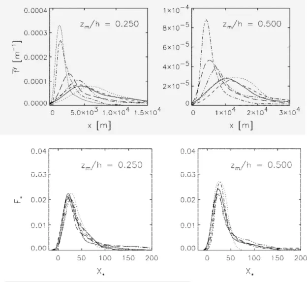
Kljun et al. (2004) have devised a simple scaling framework to determine quick estimates of cross-wind integrated

footprints for any given stability and receptor (or measurement) height,

€

x

. Basically, they use a sophisticated footprint model (Kljun et al 2002) and simulations over a wide range of stability, surface characteristics and receptor heights in order to find a suitable scaling framework for footprints. Thereby a non-dimensional footprint function,

€

F

, is introduced, which expresses the relative contribution from a non- dimensional distance,

€

X

. Figure 8.4 shows the original (dimensional) footprint functions,

€

f

, for two heights

€

x

and the corresponding non- dimensional footprint functions. As can be seen the dimensional footprints vary over order of magnitudes, while the scaling framework allows for a simple, quite general description. According to this approach the (dimensional) distance of maximum influence,

€

x

(see Fig. 8.3) can easily be estimated from

€

x

= X

x

σ

u





 





 

−α1

, (8.1)

3 Clearly, the footprint is an area on the ground rather than simply a distance. This area is often modelled to have some kind of elliptical form (Schmid 1994). A measure for only the footprint’s along-wind variation is the integration of the footprint function over the lateral dimension, i.e. the so-called cross-wind integrated footprint.

- 5 - where

€

α

= 0.8 is a (fitting) parameter and

€

X

the non-dimensional distance of the maximum impact. A parameterisation for the latter yields

€

X

≈ A

(B − ln z

) . (8.2)

€

A

= 2.59 and

€

B = 3.42 are again parameters.

Figure 8.4 Upper row: crosswind integrated flux footprints for 2 different receptor heights and varying stability conditions: strongly convective (– –), forced convective (_ · · ·), slightly convective (—), neutral (· · ·), slightly stable (- - -), stable (_·), and strongly stable (—, thin line).

€

z

denotes the receptor height,

€

x

, and

€

h the boundary layer height.

Lower row: the same simulations as in the upper row, but expressed in the non-dimensional framework

€

F * ( X * ) . Adapted from Kljun et al.

2004).

If not only the maximum of the footprint function is of interest, but also its along-wind dimension (up to which distance is there discernible surface influence to our point of interest?) the footprint function needs to be integrated. Thereby, and due to the properties of the integral, a decision must be made on what percentage of the total footprint is desired. Let

€

x

denote

- 6 -

the distance from the ‘sensor’ at which R percent of the total footprint is captured. Similar to (8.1) this (dimensional) distance can be obtained from

€

x

= X

x

σ

u





 





 

−α1

. (8.3)

€

X

may directly (i.e., graphically) be inferred from Fig. 8.5 (Kljun et al. 2004 also provide an approximate numerical solution). Evaluating eq. (8.3) and Fig.

8.5 for different stabilities and surface conditions easily shows that the often- quoted ‘rule-of-the-thumb’ (i.e., that ‘the footprint ranges up to 100 times the receptor height,

€

x

’) is indeed oversimplified and does not reflect the true variability of footprints.

Numerical models to determine footprints are usually based on some sort of

‘inversed dispersion modelling’ and will be introduced in Chapter 16.

Figure 8.5 Cumulative form of the footprint parameterization,

€

F * , as a function of the distance from the receptor,

€

X * (the hats denote the parameterization being used rather than the ‘true’ functions). Different curves discriminate between roughness lengths of z

= [0.01 (—), 0.1 (· · ·), 0.3 (_ · · ·), 1.0 (– –)] m. The right-hand panel is a zoom into the upper part of the left-hand panel.

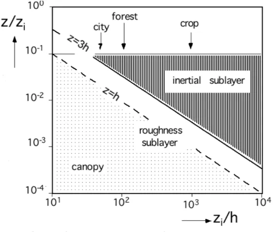
8.3 Large roughness elements

It is generally accepted that the surface layer (SL) is the layer immediately adjacent to the surface – hence its name. And it is also accepted that it comprises the lowest ten percent of the ABL. This latter characterisation comes from the original derivation for the SL being the ‘matching layer’

between an Outer Layer and an Inner Layer (see Fig. 1.3; Tennekes and Lumley 1972). However, this ‘matching’ layer, or in other words the SL has also its lower boundary, i.e.

€

x

/ z

>> 1 . Over the ideal surfaces of the early

boundary layer experiments (Fig. 8.1) and within the range of applicability of their results,

€

x

/ z

>> 1 had meant something like

€

x

> 0.1 m . Closer to surface

- 7 -

no observations were possible anyway and hence the implicit meaning ‘the surface layer is the layer adjacent to the surface’ could safely be retained.

However, when studying the turbulence structure over large roughness elements (such as trees, buildings or rocks) the ‘lower boundary’ of this layer may be some tens of meters away from the surface. Thus, beneath the surface layer there is another layer. It has become common to resolve this inconsistency in names by introducing two sub-layers of the SL: from the surface up to a height

€

z

there is a Roughness Sublayer (RS) and the reminder of the SL is called Inertial Sublayer (IS). This situation is sketched in Fig. 8.6. Note that ‘surface layer scaling’, which has become a synonym for Monin-Obukhov scaling because the latter applies to the idealised picture of the SL, is in this notation not valid within the entire surface layer but only within its upper part, i.e. the IS. Thus SL scaling applies within the IS or ‘true matching layer’ (Fig. 1.3), but not within the RS. Note also that even with very small roughness elements such as sand grains, short grass or snow crystals there is a RS, however quite shallow. The lower part of the RS, i.e. the layer that comprises the roughness elements themselves is called Canopy Layer (Fig. 8.6).

z=z_i:

≈ 1000m

z=0.1z_i:

≈ 100m

boundary layer surface layer

inertial sublayer

roughness sublayer

canopy layer

free troposphere

z≈3h z=h

height

[log scale]

Figure 8.6 Conceptual sketch and terminology for the lowest layers of the atmosphere over a rough surface. Note the logarithmic height scale.

The level

€

z

refers to the boundary layer height and h denotes the (average) height of roughness elements. From Rotach and Calanca (2002).

Figure 8.7 shows a non-dimensional picture of the layers in the boundary

layer. For small roughness elements (right end) the majority of the SL is made

up by the IS and only the lowest few centimetres belong to the RS. The larger

- 8 -

the roughness elements become (moving left in Fig. 8.7) the more important the RS becomes until it eventually covers the entire ‘lowest 10 percent’ (i.e.

the SL) of the boundary layer. Studying flows over large roughness elements – or in other words boundary layers over forested or urban surfaces – therefore largely means studying RS turbulence.

Figure 8.7 Sketch of the vertical extension of the various layers over rough surfaces and their variation with the non-dimensional quantities

€

z / z

and

€

z

/ h , where

€

z

denotes the boundary layer height and h stands for the canopy height. A value of

€

z

/ h = 3 is assumed. The arrows 'city', 'forest' and 'crop', are drawn using

€

z

= 1000m together with

€

h = 20m (city),

€

h = 10m (forest) and

€

h = 1 m (crop), respectively. These values correspond to order of magnitude estimates for the daytime (neutral to convective) boundary layer. From Rotach (1999).

Early studies of RS turbulence (e.g., Thom 1971, Garratt 1978) were performed mostly over vegetation or in wind tunnels (e.g., Raupach et al 1980) and often attempted to introducing ‘correction functions’ which had to be used in order to retain the well-known characteristics of the IS. Without going into detail we only mention here the most common ‘correction’, i.e. the introduction of a zero plane displacement,

€

d . This height responds to the fact that people found – when searching for the logarithmic part in the wind speed profile (eq. (1.8) or (4.16)) under neutral conditions - indeed a logarithmic layer, but only upon a coordinate transformation

€

x

→ x'

= x

− d . Hence, the

neutral mean wind speed profile becomes

- 9 -

€

u

(x'

) = u

k ln( x'

z

) = u

k ln( x

− d

z

) . (8.4)

In other words the flow aloft ‘sees’ an elevated (displaced) surface, which is due to the fact that a dense canopy absorbs momentum not only due to friction ‘at the ground’. In fact the zero plane displacement has been identified as the level of ‘mean momentum absorption’ (Thom 1971).

The zero plane displacement can be estimated using various methods such as fitting observations of mean wind speed to (8.4) (see Grimmond and Oke 1999 for an overview). The easiest method – and not the worst – consists in relating it to the mean obstacle height,

€

d ≈ 0.7h . Note also that the zero plane displacement is a property of the IS even if it describes a level within the RS.

In Chapter 10 the most salient features of RS turbulence for flows over vegetation and urban areas are summarised. An excellent review on RS turbulence can be found in Raupach et al (1991).

8.4 Influence of topography

Topography introduces a multitude of problems to be dealt with if the boundary layer over such surfaces is to be understood. Let us start with two very general issues. If we consider an indefinite slanted plane (again, a quite idealized type of surface) we firstly recognize that it is quite difficult in principle to define a suitable coordinate system. Figure 8.8 shows that the mere definition of the ‘vertical dimension’ poses a problem. Is it the direction normal to the surface what would be suitable if the deformation of the flow and the corresponding frictional processes were of interest? Or is it the direction of the geopotential, to which processes of buoyancy respond? Moreover, the correct coordinate system becomes an even more involved problem if the surface is not only slanted but also has changing exposition. Finnigan (2004) discusses in depths the possibilities and also the implications the choice of a coordinate system has on the frame of reference for analysing observational data.

Figure 8.8 Schematic illustration of problems inherent in defining an appropriate coordinate system over a slanted surface.

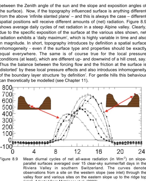
A second problem arises from the fact that the radiation a unit surface area

receives strongly depends on the inclination angle (and thus on the interplay

- 10 -

between the Zenith angle of the sun and the slope and exposition angles of the surface). Now, if the topography influenced surface is anything different from the above ‘infinite slanted plane’ – and this is always the case – different spatial positions will receive different amounts of (net) radiation. Figure 8.9 shows average daily cycles of net radiation in a steep Alpine valley. Clearly, due to the specific exposition of the surface at the various sites shown, net radiation exhibits a ‘daily maximum’, which is highly variable in time and also in magnitude. In short, topography introduces by definition a spatial surface inhomogeneity - even if the surface type and properties should be exactly equal everywhere. The same is of course true for the local pressure conditions (at least), which are different up- and downwind of a hill crest, say.

Thus the balance between the forcing flow and the friction at the surface is

‘distorted’ by these local pressure effects and also introduces inhomogeneity of the boundary layer structure ‘by definition’. For gentle hills this behaviour can theoretically be modelled (see Chapter 11).

Figure 8.9 Mean diurnal cycles of net all-wave radiation (in Wm

) on slope- parallel surfaces averaged over 15 clear-sky summer/fall days in the Riviera Valley in southern Switzerland. The curves denote observations from a site on the western slope (see inlet) through the valley floor and various sites on the eastern slope up to the ridge top (inlet). Adapted from Matzinger et al. (2003).

Both the above phenomena give rise to very characteristic flow phenomena, which are described phenomenologically here and will be discussed with their implications in some depths in Chapter 11. In valleys, on sunny convective days the development of valley and slope wind systems can generally be observed. Typically the flow is down-valley (and down-slope) during the night and up-valley (upslope) during the day with various stages of development (Fig. 8.10). These flows are triggered by differences in the thermal state of the local atmosphere between ‘the valley and the plain’ (valley wind system) and

‘the valley atmosphere and the near-slope region’ (slope wind system). For

the latter, consider the situation in Fig. 8.11, where the thermal differences are

depicted as simply two states (two different densities). Both the buoyancy and

- 11 -

the pressure gradient forces result in upslope flow (components) during the day and in down-slope flow (components) during the night. For the valley flow the situation is the same – in principle. During daytime the valley atmosphere is generally found to be warmer (smaller density) than the region at the valley entrance region (i.e., the ‘plain’, from which the valley starts), thus giving rise to up-valley winds and vice versa during the night.

Figure 8.10 Schematic representation of the various stages of the valley wind / slope wind systems during a day. a) at night; b) after sunrise; c) morning; d) noon; e) afternoon; f) early evening; g) after sunset; h) early evening. From Defant (1951).

However, there is some considerable debate as to why the valley atmosphere

should heat up (cool down) more during the day (the night). The simplest and

most intuitive explanation is the so-called Terrain Amplification Factor (TAF)

concept, first brought up by Wagner (1932) and later extended by Steinacker

- 12 -

(1984). Basically, the argument goes that for a given surface

€

A

topping a

‘box of air’ (Fig. 8.12) the box’s air volume will be smaller in the case of a valley than in the case of a plain. Hence the valley air will heat up more rapidly than the ‘plain air’ for the same amount of energy supplied from above (i.e., from net radiation). The TAF concept – although simple – has at least two serious constraints. One concerns the necessity of efficient transport of heat from the slopes to the valley centre (Weigel 2005) and the other one the fact that it assumes that there be no exchange between the ‘valley air’ and the free troposphere above. In fact, recent studies using high-resolution numerical modelling (e.g., Rampanelli et al. 2005) show that other mechanisms such as exactly this vertical exchange between the valley atmosphere and the layer aloft can lead to the heating up of the valley air alone (i.e., without the necessity of introducing the TAF) thus rendering the TAF at least as ‘not the only explanation’ for valley wind systems.

Figure 8.11 Schematic illustration of the forcing mechanisms of thermally driven

slope winds. The near-surface layer next to the slope heats up (cools

down) more during the day (at night) than does the air over the valley

center. The arising density gradients induce buoyancy and horizontal

pressure gradient forces. Their slope-parallel components (encircled)

lead to the development of daytime up-slope flow (a) and nocturnal

down-slope winds (b).

- 13 -

Figure 8.12 Illustration of the TAF concept and the associated volumes of a valley, a) and a plain, b). From Weigel (2005).

Dynamically the introduction of topography leads to a convergence of the flow over the crest and hence to speed up there. Downwind of the crest in the wake region of the hill the flow is decelerated (Fig. 8. 13). Whether or not a

‘separation bubble’ forms, where the flow is actually reversed, depends on the steepness of the terrain. The associated boundary layer structure becomes more complicated and requires the introduction of additional layers as discussed in Chapter 11. It should be noted that all our current theoretical knowledge concerning flow over topography is essentially constrained to gentle hills. The associated theory is based on linearization of the problem (see Chapter 11 and the pioneering work of Jackson and Hunt 1975) and can therefore not be applied over hills with slopes of more than some 15°.

Figure 8.13: Schematic of the flow structure over a low hill (left) and the associated

profiles of mean wind speed at different positions. ‘l’ in the right vertical

axis denotes the half-width of the hill. From Kaimal and Finnigan

(1994).

- 14 -

Apart from theoretically studying flows over gentle hills they have frequently been studied in wind tunnels (e.g., Finnigan et al. 1990) and even in full-scale experiments. One of the landmark studies in this respect certainly was the

‘Askervein Hill’ project (Taylor and Teunissen 1987), in which the theoretical understanding of the linear theory was challenged against field observations.

Figure 8.14 Photograph of Askervein Hill located on the southern part of the wes coast of South Uist, one of the Islands of the Scottish Outer Hebrides.

From http://www.yorku.ca/pat/research/Askervein/.

With respect to flows over really complex terrain such as in the Alps the

Rockies or the Himalayas, relatively little is known concerning the full

boundary layer structure including turbulence. Most studies so far have

concentrated on valley and slope wind systems and mean flow characteristics

(e.g., Whiteman 1990, 2000; Egger et al. 2000). Details of the turbulence

state in the boundary layer over highly complex terrain have only started to

evolve from very recent field campaigns such as VTMX (Vertical Transport

and Mixing) in the Salt Lake Valley (Doran et al 2002) and MAP Riviera

(Rotach et al. 2004) and associated numerical modelling studies (e.g. Zhong

and Fast 2003; DeWekker et al. 2005; Zängl et al. 2001).

- 15 -

References Chapter 8

Chow, FK and Street RL: 2004, Evaluation of turbulence models for Large-Eddy simulations of flow over Askervein hill; Preprints 16^th AMS Symposium on Boundary Layers and Turbulence, Vancouver, CA, paper 7.11, 8pp

Clarke, R.H., et al., 1971: The Wangara experiment: Boundary layer data. Tech. Paper, 19, Div. Meteor, Phys. CSIRO, Australia.

Defant, F.: 1951, Local winds. Compedium of Meteorlogy, T. Malone, Ed., American Met.

Soc, Boston.

DeWekker SJF, Steyn DG, Fast JD, Rotach MW and ZhongS: 2005, Convective boundary layer structure and RAMS performance in a very steep valley, Environ. Fluid Mech. 5, 35-62.

Doran, J. C., J. D. Fast, and J. Horel: 2002, The VTMX 2000 campaign. Bull. American Met.

Soc., 83, 537–551.

Egger, J., S. Bajrachaya, U. Egger, R. Heinrich, J. Reuder, P. Shayka, H. Wendt, and V.

Wirth: 2000: Diurnal winds in the Himalayan Kali Gandaki Valley. Part I: Observations.

Mon. Wea. Rev., 128, 1106–1122.

Finnigan JJ: 2004, A Re-Evaluation of Long-Term Flux Measurement Techniques Part II:

Coordinate Systems, Boundary-Layer Meteorology, 113, 1-41.

Finnigan JJ, Raupach MR, Bradley EF and Aldiss GK: 1990, A wind-tunnel study of turbulent flow over a a two-dimensional ridge, Boundary-Layer Meteorol, 50, 277-317.

Garratt, J.R.: 1978, Flux-profile relationships above tall vegetation, Quart J Roy Meteorol Soc, 104, 199-211.

Grimmond, C.S.B. and Oke, T.R.: 1999, ‘Aerodynamic Properties of Urban Areas Derived from Analysis of Surface Form’, J. Appl. Meteorol., 38, 1262–1292.

Haugen DA, Kaimal JC and Bradley EF: 1971, An experimental study of Reynolds stress and heat flux in the atmospheric surface layer, Quart J Roy Meteorol Soc, 97, 168-180.

Jackson PS and Hunt JRC: 1975, Turbulent wind low over a low hill, Quart J Roy Meteorol Soc, 101, 929-955.

Kljun, N.; Rotach, M.W. and Schmid, H.P.: 2002, 'A 3D Backward Lagrangian Footprint Model for a Wide Range of Boundary Layer Stratifications', Boundary-Layer Meteorology, 103, 205-226.

Kljun, N; Calanca, P. Rotach, M.W. and Schmid, H.P.: 2004, ‘A simple parameterization for flux footprint predictions’, Boundary-Layer Meteorology 112: 503–523.

Matzinger, N.; Andretta, M., van Gorsel, E.; Vogt, R.; Ohmura, A. and Rotach, M.W: 2003, 'Surface Radiation Budget in an Alpine Valley', Quarterly J. Roy. Meteorol. Soc., 129, 877-895.

Rampanelli, G., D. Zardi, and R. Rotunno: 2005, Mechanisms of up-valley winds, J. Atmos.

Sci. , 61, No. 24, 3097–3111.

Raupach , M.R.; Thom, A.S. and Edwards, I.: 1980, A wind-tunnel study of turbulent floow close to regularly arrayed rough surfaces, Boundary-Layer Meteorol, 18, 373-397.

- 16 -

Raupach M.R., Antonia R.A. and Rajagopalan S.: 1991, ‘Rough-Wall Turbulent Boundary Layers’, Appl. Mech. Rev., 44, pp 1-25.

Rotach, M.W.: 1999, 'On the Influence of the Urban Roughness Sublayer on Turbulence and Dispersion', Atmospheric Environ, 33, 4001–4008.

Rotach, M.W. and Calanca, P.: 2002, ‘Microclimate’, in Holton, J.C., Pyle, J and Curry, J.A.

(Eds.), ‘Encyclopaedia of Atmospheric Sciences’, Academic Press, 1301-1307.

Rotach, M. W., P. L. Calanca, R. Vogt, D. Steyn, G. Graziani, M. Andretta, A. Christen, S.

Cieslik, R. Conolly, S. Galmarini, E. van Gorsel, J. Gurtz, E. Kadygrov, V. Kadygrov, E.

Miller, B. Neininger, M. Rucker, H. Weber, A. Weiss, S. de Wecker, and M. Zappa, 2004: The turbulence structure and exchange processes in an Alpine valley: The Riviera project. Bull. Amer. Meteor. Soc., 85, 1367–1385.

Schmid, H. P.: 1994, ‘Source Areas for Scalars and Scalar Fluxes’, Boundary-Layer Meteorol.

67, 293–318.

Schmid, H. P.: 2002, ‘Footprint Modeling for Vegetation Atmosphere Exchange Studies: A Review and Perspective’, Agric. For. Meteorol. 113, 159–184.

Steinacker, R. 1984, Area-height distribution of a valley and its relation to the valley wind.

Contrib. Atmos. Phys., 57, 64–71.

Tennekes, H. and Lumley, J.J.: 1972, A first course in turbulence, MIT Press, 300pp.

Taylor PA and Teunissen HW: 1987, The Askervein project: overview and background data, Boundary-Layer Meteorology, 39, 15-39.

Thom, A.S.: 1971, Momentum absorption by tall vegetation, Quart J Roy Meteorol Soc, 97, 414-428.

Wagner, A.: 1932, Der tägliche Luftdruck- und Temperaturgang in der freien Atmosphäre und in Gebirgstälern. Gerl. Beitr. Geophys., 37, 315–344.

Whiteman, C. D.: 1990, Observations of thermally developed wind systems in mountainous terrain, Atmospheric processes over complex terrain,W. Blumen, ed., AmericanMet.

Soc., Boston, 5–42.

Whiteman, C. D.: 2000, Mountain Meteorology. Fundamentals and applications, Oxford University Press, NewYork, Oxford.

Weigel, AHP: 2005, On the atmospheric boundary layer over highly complex topography, ETH Diss. No 15972, 175 pp.

Zängl, G., J. Egger, and V.Wirth: 2001, Diurnal winds in the Himalayan Kali Gandaki Valley.

Part II: Modeling. Mon. Wea. Rev., 129, 1062–1080.

Zhong, S. and J. Fast: 2003, An evaluation of the MM5, RAMS, and Meso-Eta models at subkilometer resolution using VTMX field campaign data in the Salt Lake Valley. Mon.

Wea. Rev., 131, 1301–1322.