Time Resolved Measurements of the Switching Trajectory of Pt=Co Elements Induced by Spin-Orbit Torques

Time Resolved Measurements of the Switching Trajectory of Pt=Co Elements Induced by Spin-Orbit Torques

M. M. Decker,¹ M. S. Wörnle,¹ A. Meisinger,¹ M. Vogel,¹ H. S. Körner,¹ G. Y. Shi,² C. Song,² M. Kronseder,¹ and C. H. Back¹

1Department of Physics, Regensburg University, 93053 Regensburg, Germany

2Key Laboratory of Advanced Materials (MOE), School of Materials Science and Engineering, Tsinghua University, Beijing 100084, China

(Received 14 March 2017; published 22 June 2017)

We report the experimental observation of spin-orbit torque induced switching of perpendicularly magnetized Pt=Co elements in a time resolved stroboscopic experiment based on high resolution Kerr microscopy. Magnetization dynamics is induced by injecting subnanosecond current pulses into the bilayer while simultaneously applying static in-plane magnetic bias fields. Highly reproducible homogeneous switching on time scales of several tens of nanoseconds is observed. Our findings can be corroborated using micromagnetic modeling only when including a fieldlike torque term as well as the Dzyaloshinskii-Moriya interaction mediated by finite temperature.

DOI:10.1103/PhysRevLett.118.257201

Magnetization switching induced by spin-orbit torques (SOTs) generated by in-plane (IP) current pulses in ferromagnetic (FM)/heavy metal (HM) bilayers has attracted great attention in recent years [1–17]. A typical structure comprises a FM element with perpendicular magnetization structured on top of a HM conductor carrying the current. Technologically, such a device has the advantage that the write current causing magnetization switching does not have to pass through a potential memory element itself, thus avoiding its degradation[18]. Studying magnetization dynamics in such elements is of interest since the exact mechanisms enabling deterministic mag- netization reversal remain to be disentangled. SOT driven magnetization reversal in HM/FM bilayers originates from a combination of effects which manifest themselves as field- and dampinglike torques. These torques arise from bulk and interface effects such as the bulk spin Hall effect (SHE) or the interfacial inverse spin Galvanic effect. Recent efforts have been dedicated to the understanding of the switching process induced by static or quasistatic currents [1,2,4,5,10,15,19]. However, the nature of the switching process itself is still under debate. Two possible scenarios exist: coherent rotation [4] and domain nucleation and propagation [2]. The critical current densities required for these distinct processes differ by orders of magnitude since, for domain driven reversal, a much smaller energy barrier needs to be overcome. It is believed that, for devices much larger than one domain wall width, the quasistatic switch- ing process is domain driven [2,5,9,15]. However, when reducing the size, it has been demonstrated recently that the switching process can be described by uniform motion [14]. By studying switching probabilities using short current pulses of variable width[3,6,7,14], reliable switch- ing for applied pulse widths as short as 180 ps[6]has been

demonstrated. In these experiments, switching dynamics has been investigated indirectly by examining the final state long after the current pulse has been applied. To understand the speed and type of the SOT induced switching process in detail, temporal and spatial resolution is required which is met in this Letter using time resolved scanning magneto- optical Kerr micoscopy (TRMOKE).

Here, we measure the trajectory of the magnetization of perpendicularly magnetized Pt=Co elements during rever- sal using a pump-probe approach. We observe magnetiza- tion reversal on a time scale of tens of nanoseconds mediated by domain wall motion. By comparison with micromagnetic simulations, we identify the importance of both the Dzyaloshinskii-Moriya interaction (DMI) and the fieldlike torque for the switching process.

2×2μm²Co squares on top of a2μm wide,20μm long Pt line are prepared from a stack of Tað3nmÞ=Ptð8.5nmÞ=

Coð0.5nmÞ=Al₂O₃ð5nmÞgrown onto thermally oxidized, highly resistive silicon by molecular beam epitaxy. The square is integrated into a50Ωmatched Au microstrip to ensure a good transmission of short current pulses. To study the dependence of size and shape, samples with 750 nm diameter disks have been prepared on top of the2μm wide Pt line. The results obtained for the two geometries do not differ significantly[20].

To calibrate the TRMOKE experiments, we record hys- teresis loops in the center of a2×2 μm²square sample in a not time resolved measurement, but by using the same laser system. Figure 1(c) shows two measurements performed statically. The upper panel shows a typical hysteresis curve.

The lower panel shows quasistatic current induced switching in an applied IP field ofBx¼−20mT. The input current is a square signal of 0.5 Hz with a current density of 4×10¹⁰ A=m². Both measurements give access to the 0031-9007=17=118(25)=257201(5) 257201-1 © 2017 American Physical Society

absolute Kerr signal of about 150 mdeg resulting from complete magnetization reversal enabling calibration of the signals acquired in time resolved measurements.

Magnetization dynamics is measured using a pump- probe TRMOKE experiment with≈500nm resolution, as sketched in Fig.1(b) and described in detail in Ref.[20].

In this stroboscopic experiment, the current pulse train of alternating positive and negative pulses is generated using two pulse generators which are triggered by the laser pulses and by combining their outputs. The resulting pulse train is then amplified by a broadband amplifier. Using a combi- nation of electrical and optical delay lines, we adjust the

delay between probing pulse and current pulse at the position of the sample with a timing jitter of∼50ps over a full period of 200 ns, as shown in Fig.1(d). Here, 1 ns wide pulses with a peak current density of jmax¼3.1× 10¹² A=m²are used to switch the magnetization in a static magnetic field ofBx ¼−50mT. Starting from the“down state,”the positive pulse toggles the magnetization to the

“up state”and the negative pulse back down, as expected for the layer sequence and a positive spin Hall angle in Pt.

The switching process of a perpendicularly magnetized ferromagnet can be understood when solving the Landau- Lifshitz-Gilbert (LLG) equation[2,4,13,21]

∂m

∂t ¼−γm×μ₀Heffþαm×∂m

∂t

þγτDLm×ðm×yÞ−γτFLm×y: ð1Þ Here,mdenotes the unit vector of the magnetization,γ¼ 180rad=ðTsÞis the gyromagnetic ratio, andαis the Gilbert damping parameter.Heff is the effective field given by the vector sum of the externally applied magnetic field Hext

and the effective out-of-plane (OOP) field HOOP¼

½2K^⊥=ðμ₀M_sÞ−M_sm_z, with the saturation magnetization Msand the uniaxial perpendicular anisotropy constantK^⊥. The effect of the SOTs is taken into account via the last two terms, which are called damping- (TDL) and field- (TFL) like SOTs, respectively. In the picture of the SHE, the strength of the dampinglike torque can be expressed as τDL¼ℏ=ð2jejÞΘeffjc=ðMsdFÞ, with the effective spin Hall angleΘeff[2,13], the ferromagnetic layer thicknessdF, and the injected current densityj_cjjx. Forj_c>0, the injected moment μin points in the −y direction for our geometry [22]. In the case of a full micromagnetic simulation, Heff

also includes the exchange interaction (A¼10⁻¹¹ J=m), and an additional DMI term which is known to be present in asymmetrically sandwiched Pt=Co=oxide layers and is essential for reproducible domain formation [23]. For deterministic bipolar switching, the combination of a dampinglike SOT and an additional IP field perpendicular toyis crucial[2,6]. The IP field breaks the symmetry of the magnetic response toTDLsince it exerts a torque tomthat adds to TDL in one half sphere and counteracts it in the other half sphere.

In the simplest case, i.e., for coherent rotation and neglecting TFL, the switching current can be determined analytically fromτDL;crit ¼ ðμ₀=2ÞðHOOP− ffiffiffi

p2

HextÞ[4,6].

In this case, the dynamics can be calculated by numerically solving the LLG for a given set of parameters. Examples are shown in Figs.1(e)and1(f)for a 500 ps long pulse and two different IP fieldsHx¼0.02×HOOP(the red curves) andHx¼0.2×HOOP(the blue curves). Figure1(e)shows that the magnetization switches within the first 100 ps (250 ps) for the larger (smaller) field value. The damping- like torque is chosen such thatτ_DL;max¼ ðμ₀HOOP=2Þandα is set to 0.5[23,24]. In Fig.1(f)the 3D trajectory ofmðtÞ for the larger field value is shown, whereas in Fig.1(e)the FIG. 1. (a) Colored scanning electron microscopy image of the

device. The 2×2μm² Pt=Co element is marked in blue. The inset sketches the layer system. (b) A simplified block diagram of the experimental setup. (c) Static polar Kerr measurements recorded in the center of the element. (Upper panel) Hysteresis curve. (Lower panel) Quasistatic current induced magnetization reversal forBx¼−20mT andjPt¼ 4×10¹⁰A=m². (d) Time resolved measurement of magnetization reversal for Bx¼

−50mT. (Lower panel, green curve) Current pulse train as transmitted through the sample. (Upper panel, blue curve) TRMOKE signal obtained by scanning the delay δt between the current and laser pulses. The signal is recorded for one period (200 ns) and is repeated to elucidate the measurement technique.

(e),(f) Numerical solution of the LLG equation for a 500 ps current pulse (green curves) creating a SOT strong enough to pull the magnetization into the plane. Two cases for different external fields are shown, Hx¼ þ0.02HOOP (red curves) and Hx¼ þ0.2HOOP(blue curves). (e) shows thezcomponent only, while (f) shows the 3D trajectory.

time evolution of mz is plotted. In Fig. 1(f) the torques resulting from the fields and the SOT are shown to elucidate the role of the IP field. Note that the switching time itself strongly depends on the strength and rise time of the pulse, as was worked out in Ref. [13].

Simplified macrospin calculations are illustrative, but they fail to explain the switching process quantitatively and even qualitatively, as we will detail below. This can have multiple origins. (i) A nonzero fieldlike torqueTFLreduces the critical current; the strength and sign of this torque strongly influence the dynamics [13,14]. (ii) It is known that switching is thermally assisted. The influence of thermal fluctuations leads to a strong dependence of the critical current on the pulse length. Note that thermal activation can be included in a macrospin calculation [10,25–27]. (iii) For magnetic ele- ments with dimensions large enough to accommodate a domain wall, the reversal process can be driven by domain nucleation and propagation, further reducing the energy barrier. For a Pt=Co bilayer, this has first been described in Ref. [2], where a model is used that implicitly includes thermal activation and domain driven switching for static currents. Subsequently, experiments using pulsed currents of variable pulse widthτp have been reported discussing the effects of thermal activation [3,6,8,10,14] and device size [14]on the switching mechanism.

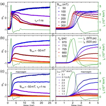
To gain insight into the mechanisms at work, we study the reversal process as a function of time. In Fig.2the Kerr signal recorded in the middle of the element is displayed. The left graphs show the full recorded time span of 25 ns; the right ones are enlarged to the first 5 ns only. Figure2(a) shows the time evolution of m_z for different applied fields whereHext< HOOP. The fixed current pulse shown in green reaches a peak current densityjmax ¼3.1×10¹²A=m², with τ_p¼1ns. The switching process is slowest for the lowest field and speeds up as the field is increased, as expected from theory. For field values whenHext≫Hcrit, the magnetization switches back to the initial equilibrium position mz¼−1 subsequent to the pulse. In Fig.2(b)the pulse width is varied between 600 ps and 1 ns for a fixedBext¼−50mT and an almost constant jmax. For τp<1ns the critical current density cannot be reached, leading to a fast decrease of the switching probability. This is seen as a reduced“up level,” e.g., forτp¼770ps where the magnetization switches with about 80% probability and the signal recorded is 0.8m_z− 0.2m_z¼0.6m_z due to statistical averaging of the pump- probe technique. For even shorter pulses whereτ_p≤700 ps, we observe only a small canting ofmfrom the equilibrium state and subsequent relaxation. Similar results are found when reducing the peak amplitude of the current pulse at a fixed Bext¼−50mT and τp¼1ns; see Fig. 2(c). Addi- tional measurements at high fields are shown in Ref.[20].

Making use of the spatial resolution of TRMOKE, images of the switching process are taken to investigate possible spatial inhomogeneities during reversal. An example for τ_p¼1ns,Bext ¼−50mT, andjmax¼3.1×10¹² A=m²is shown in Fig.3. Figure3(a)shows the switching curve in

blue. The inset shows the reflected intensity where the current contacts (yellow) can be seen on the left and right sides. The images shown in Fig.3(b)are snapshots of the reversal at times marked with red dots in Fig. 3(a). The switching process is homogeneous without the appearance of propagating domains. The same result is found at different jmax’s and external fields. In Ref.[23], the switching of a 100 nm diameter disk has been simulated, and it is predicted that the switching occurs via deterministic domain nucleation at one side of the disk and subsequent domain wall propagation across the disk under the influence of the current.

0

-1 1

0 3

1 2

jc (1012 A/m2) mz

0

-1 1

jc (1012 A/m2) 0 3

1 2

jc (1012 A/m2) 0

-1 1

0 3

1 2

0 5 10 15 20 25 0 1 2 3 4 5

(a)

(b)

(c)

Bext (mT):

p=1.ns

50 100 150 200 250 300

p (ps): 970 770 705 660 620 B_ext = -50.mT

j_c(970 ps) j_c(620 ps)

Bext = -50^.mT, p=1^.ns

jmax (10¹² A/m²):

3.1 2.8 2.5 2.2 2.0 1.6 1.1 3.1

macrospin macrospin

time (ns) time (ns)

mzmz

LLG

FIG. 2. Transient normalized magnetization mzðtÞ (symbols, left axis) and current densityjcðtÞ(green solid lines, right axis) as a function of delay time. The right graphs show the first 5 ns of the respective left graphs in detail. (a) Magnetization reversal forτp¼1ns andBextranging from−50to−300mT at a fixed jmax¼3.1×10¹² A=m². For large fields the magnetization relaxes back into the initial equilibrium position after the switch- ing event. (b) Measurements for a fixed Bext¼−50mT and different pulse durationsτpranging from 0.6 to 1 ns. (c) Current density dependence forτp¼1ns andBext¼−50mT. Numeri- cal solutions of the LLG in comparison to the experiment are shown as solid lines.

0 1

-1

0 5 10

time (ns)

mz

reflectivity

1.0 ns 2.5 ns

4.0 ns 10.0 ns

mz 0 0.6

-0.6

(a) _j (b)

max = 3.1×10^12.A/m² B_ext = -50.mT

p=1 ns

FIG. 3. (a) mzðtÞ trace recorded in the middle of the sample.

The inset shows the reflectivity (topography). (b) Images of the switching process taken at distinct times shown in red in (a).

It is also shown that the nucleation point is determined by the shape of the magnetic element in combination with the presence of DMI. Such a scenario must be visible using our experimental technique if the process is deterministic. To ensure that our results are not caused by the shape of the sample, a disk shaped sample with a diameter of 750 nm was measured. The results do not differ significantly from the presented data[20].

To obtain a quantitative understanding of the experimental results, Eq.(1)is solved numerically using the predetermined M_sandK^⊥, neglectingTFLand thermal effects, sinceτ_p≤ 1ns is below the thermally activated regime [6,10,25,26].

Forτp¼1ns andjc¼3.1×10¹²A=m², atBext¼−50mT, switching is achieved for aτDLvalue leading toΘeff ¼0.13, which is in good agreement with published experimental results in similar structures[6,28]; i.e. the switching current itself can, in principle, be explained by a simple LLG calculation. However, the time scale of the switching process differs from the measured data, as shown in Fig.2(c). The solid blue lines show the numerical solution corresponding to the measured data forjmax¼3.1×10¹²A=m², which is shown in dark blue symbols. In the measurement the full level m_z¼1 is reached aftert≈30ns, in contrast to the much faster switching in the calculation. We emphasize that, within the macrospin model, the switching process must occur within the pulse duration due to the combination of a large value forαand the relatively long rise and fall times of the pulse. This statement still holds if a nonzero TFL or thermal activation is added to the LLG. However, 1 ns pulses in the10¹² A=m²regime are likely to heat up the element by some 10–100 K, which may significantly influence the magnetic properties, such as Ms. To estimate the impact of a temperature increase, measurements of MsðTÞ are performed [20]. A Curie temperature of TC≈400 K is found which agrees with previous reports[29]. To examine whether Joule heating of the sample could explain the long signal recovery times, finite elementsCOMSOL®simulations are performed to investigate how rapidly the element cools down after the pulse has passed. We find that the temperature recovers its initial value in<7ns after the pulse ends. Thus, the magnetic signal should be recovered after this time. It should be noted that the peak temperature of the sample remains well below TC since demagnetization of the Co layer, which would manifest itself as a plateau in the Kerr data, is not observed. We conclude that a macrospin approach, even when considering Joule heating, cannot adequately explain our results.

To further investigate our finding that the reversal process appears homogeneous but does not follow a macrospin model, micromagnetic simulations are performed using MUMAX³[30]. The material parameters used are the same as for the LLG calculations but include DMI as well. The strength of the DMI has been measured frequently in Pt=Co=oxide systems; DMI constants range fromDdCo∼ 0.3pJ=m[9,31]to∼2pJ=m[32–34]. In our simulations, a DMI constant of DdCo¼0.5pJ=m is assumed. Larger

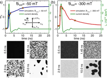
values lead to multidomain states in zero field due to the relatively lowHOOP of our samples and the fact that DMI greatly reduces the cost of the domain walls. In Figs.4(a) and4(b), simulation results for two fields,−50and−300 mT, are shown. The two upper graphs show the averaged magnetization as a function of time. The lower panels show snapshots at distinct times marked by dots in the upper traces.

In the simulation the magnetic field is tilted OOP by 1° from thexaxis such thatH <0→Hz<0, leading to a relaxation back into the stable equilibrium for large fields, as seen in the experiment. The similarity of the simulated and measured curves is striking. Especially interesting is the fact that the slow switching time can be reproduced for the−50mT case.

Most importantly we find that the experimental results can be reproduced only if DMI, a fieldlike torqueτFL, and finite temperatures (100 K) are taken into account.

The result closest to the measurement is reached for τFL=j_c ¼0.045 pT m²=A and τDL=j_c ¼0.067 pT m²=A, which is close to the literature values in[35]. The sign of τFLis such thatTFLandTDLtry to align the magnetization in opposite directions; in this case,TFLdestabilizes the system during the pulse. Together with the finite temperature, small domains are continuously created and annihilated during the duration of the pulse. These then relax into the new state only after the pulse is turned off. The nucleation happens in a random fashion. In the simulation, it depends on the seed of the random field used to implement temperature. If measured by a stroboscopic technique, the statistical average over many switching events results in a homogeneous value across the sample, corroborating the results shown in Fig.3. Without DMI, this relaxation happens much faster than seen in the experiment. This scenario is observed when τFL dominates overBext. ForjBextj≥100mT, the external field stabilizes the system and speeds up the reversal process.

However, owing to the lowHOOPandHcritin our system, the

jc (1012 A/m2) 0

-1 1

0 5 10 15 20 25

time (ns) mz

0 5 10 15 20 25

0.5 ns 1.45 ns

2.9 ns 10.0 ns

time (ns) 0

-1 1

1 0 2 3

1 0 2 3

current density simulation, B

ext,x

current density simulation, B

ext,x

B_ext= -50 mT B_ext= -300 mT

= -50 mT = -300 mT

x,jc Hext

y, ,HFL

µin,TDL Mstart

0.5 ns 1.85 ns

2.9 ns 10.0 ns

(a) (b)

FIG. 4. Micromagnetic simulations of the switching process for 2μm wide squares using IP field values of (a) −50 and (b)−300 mT to model the data shown in Fig.2(a). (Upper panels) Time evolution ofmz. Orange dots denote the times for which snapshots are shown in the lower part of the figure.

new state is not stable, such that the subsequent relaxation process overlays the switching process. For a detailed analysis of the contributions of DMI and τFL (including different signs), see Ref.[20].

In conclusion, we have recorded time resolved microscopic images of the SOT induced switching process of micron sized Pt=Co elements. We have shown that, in order to explain our results, the temperature, DMI, and fieldlike torque have to be taken into account. For the case shown here, switching occurs by the nucleation of domains. Surprisingly—and mediated by the combined action of the DMI and fieldlike torque—the switching process takes much longer than the pulse duration. Note that, for different parameter sets (particularly large OOP anisotropies), the switching process can be described by the nucleation and propagation of a domain within the current pulse duration[23].

We would like to acknowledge the DFG for funding via Grant No. SFB 689 and the group of P. Gambardella for sharing their data prior to publication.

Note added.—Recently, two papers appeared addressing similar issues[36,37].

[1] I. M. Miron, K. Garello, G. Gaudin, P.-J. Zermatten, M. V.

Costache, S. Auffret, S. Bandiera, B. Rodmacq, A. Schuhl, and P. Gambardella,Nature (London)476, 189 (2011).

[2] L. Liu, O. J. Lee, T. J. Gudmundsen, D. C. Ralph, and R. A.

Buhrman,Phys. Rev. Lett.109, 096602 (2012).

[3] C. O. Avci, K. Garello, I. M. Miron, G. Gaudin, S. Auffret, O. Boulle, and P. Gambardella, Appl. Phys. Lett. 100, 212404 (2012).

[4] K.-S. K.-J. Lee, S.-W. Lee, B.-c. Min, and K.-S. K.-J. Lee, Appl. Phys. Lett.102, 112410 (2013).

[5] S. Emori, U. Bauer, S.-M. Ahn, E. Martinez, and G. S. D.

Beach,Nat. Mater. 12, 611 (2013).

[6] K. Garello, C. O. Avci, I. M. Miron, M. Baumgartner, A. Ghosh, S. Auffret, O. Boulle, G. Gaudin, and P.

Gambardella,Appl. Phys. Lett.105, 212402 (2014).

[7] M. Cubukcu, O. Boulle, M. Drouard, K. Garello, C. O.

Avci, I. M. Miron, J. Langer, B. Ocker, P. Gambardella, and G. Gaudin,Appl. Phys. Lett.104, 042406 (2014).

[8] C. Bi, L. Huang, S. Long, Q. Liu, Z. Yao, L. Li, Z. Huo, L.

Pan, and M. Liu,Appl. Phys. Lett.105, 022407 (2014).

[9] O. J. Lee, L. Q. Liu, C. F. Pai, Y. Li, H. W. Tseng, P. G.

Gowtham, J. P. Park, D. C. Ralph, and R. A. Buhrman, Phys. Rev. B89, 024418 (2014).

[10] K. S. Lee, S. W. Lee, B. C. Min, and K. J. Lee,Appl. Phys.

Lett.104, 072413 (2014).

[11] J. Torrejon, F. Garcia-Sanchez, T. Taniguchi, J. Sinha, S.

Mitani, J. V. Kim, and M. Hayashi,Phys. Rev. B91, 214434 (2015).

[12] G. Yu, P. Upadhyaya, Y. Fan, J. G. Alzate, W. Jiang, K. L.

Wong, S. Takei, S. A. Bender, L.-T. Chang, Y. Jiang, M.

Lang, J. Tang, Y. Wang, Y. Tserkovnyak, P. K. Amiri, and K. L. Wang,Nat. Nanotechnol.9, 548 (2014).

[13] W. Legrand, R. Ramaswamy, R. Mishra, and H. Yang,Phys.

Rev. Applied3, 064012 (2015).

[14] C. Zhang, S. Fukami, H. Sato, F. Matsukura, and H. Ohno, Appl. Phys. Lett.107, 012401 (2015).

[15] C. J. Durrant, R. J. Hicken, Q. Hao, and G. Xiao,Phys. Rev.

B 93, 014414 (2016).

[16] S. Fukami, C. Zhang, S. DuttaGupta, A. Kurenkov, and H.

Ohno,Nat. Mater. 15, 535 (2016).

[17] P. Li, T. Liu, H. Chang, A. Kalitsov, W. Zhang, G. Csaba, W. Li, D. Richardson, A. DeMann, G. Rimal, H. Dey, J. S. Jiang, W.

Porod, S. B. Field, J. Tang, M. C. Marconi, A. Hoffmann, O.

Mryasov, and M. Wu,Nat. Commun.7, 12688 (2016).

[18] K. Ando, S. Fujita, J. Ito, S. Yuasa, Y. Suzuki, Y. Nakatani, T.

Miyazaki, and H. Yoda,J. Appl. Phys.115, 172607 (2014).

[19] G. Yu, P. Upadhyaya, K. L. Wong, W. Jiang, J. G. Alzate, J.

Tang, P. K. Amiri, and K. L. Wang,Phys. Rev. B89, 104421 (2014).

[20] See Supplemental Material at http://link.aps.org/

supplemental/10.1103/PhysRevLett.118.257201 for a de- tailed description of the measurement setup and sample design as well as for additional data and simulation results.

[21] J. Slonczewski,J. Magn. Magn. Mater.159, L1 (1996).

[22] J. E. Hirsch,Phys. Rev. Lett.83, 1834 (1999).

[23] N. Mikuszeit, O. Boulle, I. M. Miron, K. Garello, P.

Gambardella, G. Gaudin, and L. D. Buda-Prejbeanu,Phys.

Rev. B92, 144424 (2015).

[24] S. Mizukami, E. P. Sajitha, D. Watanabe, F. Wu, T. Miyazaki, H. Naganuma, M. Oogane, and Y. Ando,Appl. Phys. Lett.

96, 152502 (2010).

[25] D. Bedau, H. Liu, J. Z. Sun, J. A. Katine, E. E. Fullerton, S.

Mangin, and A. D. Kent,Appl. Phys. Lett.97, 262502 (2010).

[26] H. Liu, D. Bedau, J. Z. Sun, S. Mangin, E. E. Fullerton, J. A.

Katine, and A. D. Kent,J. Magn. Magn. Mater. 358–359, 233 (2014).

[27] M. Lederman, S. Schultz, and M. Ozaki,Phys. Rev. Lett.73, 1986 (1994).

[28] W. Zhang, W. Han, X. Jiang, S.-H. Yang, and S. S. P. Parkin, Nat. Phys.11, 496 (2015).

[29] T. Koyama, A. Obinata, Y. Hibino, A. Hirohata, B.

Kuerbanjiang, V. K. Lazarov, and D. Chiba, Appl. Phys.

Lett.106, 132409 (2015).

[30] A. Vansteenkiste, J. Leliaert, M. Dvornik, M. Helsen, F. Garcia-Sanchez, and B. Van Waeyenberge, AIP Adv.

4, 107133 (2014).

[31] M. J. Benitez, A. Hrabec, A. P. Mihai, T. A. Moore, G.

Burnell, D. McGrouther, C. H. Marrows, and S. McVitie, Nat. Commun.6, 8957 (2015).

[32] N. H. Kim, D. S. Han, J. Jung, J. Cho, J. S. Kim, H. J. M.

Swagten, and C. Y. You, Appl. Phys. Lett. 107, 142408 (2015).

[33] C. F. Pai, M. Mann, A. J. Tan, and G. S. D. Beach, Phys.

Rev. B93, 144409 (2016).

[34] M. Belmeguenai, J. P. Adam, Y. Roussigné, S. Eimer, T.

Devolder, J. V. Kim, S. M. Cherif, A. Stashkevich, and A.

Thiaville,Phys. Rev. B91, 180405(R) (2015).

[35] K. Garello, I. M. Miron, C. O. Avci, F. Freimuth, Y.

Mokrousov, S. Blügel, S. Auffret, O. Boulle, G. Gaudin, and P. Gambardella,Nat. Nanotechnol.8, 587 (2013).

[36] M. Baumgartneret al.,arXiv:1704.06402.

[37] J. Yoon, S. W. Lee, J. H. Kwon, J. M. Lee, J. Son, X. Qiu, K. Ji. Lee, and H. Yang, Sci. Adv.3, e1603099 (2017).