Worksheet 5: Charge Distribution Around a Charged Rod

Simulation Methods in Physics II SS 2019

Worksheet 5: Charge Distribution Around a Charged Rod

Kartik Jain, David Sean, Olaf Lenz and Mehmet Süzen Institute for Computational Physics, University of Stuttgart

Contents

1 Introduction 2

2 Short Questions - Short Answers 2

3 The Simulated System 2

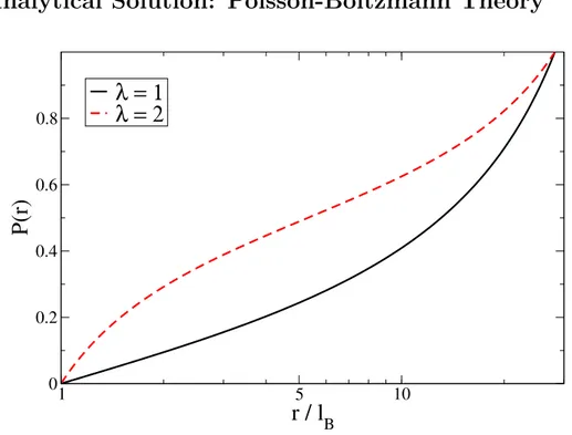
4 Analytical Solution: Poisson-Boltzmann Theory 3

5 Computer simulations 4

5.1 Mapping the Cell Model onto a Simulation . . . . 4

5.2 Warmup Runs . . . . 5

5.3 Equilibration and Sampling Time . . . . 6

5.4 Measuring the Charge Distribution . . . . 7

Bibliography 8

General Remarks

• Deadline for the report is Wednesday, 3rd of July 2019, 12:00 noon

• In this worksheet, you can achieve a maximum of 20 points.

• The report should be written as though it would be read by a fellow student who attends the lecture, but doesn’t do the tutorials.

• To hand in your report, send it to your tutor via email.

– Kartik (kartik.jain@icp.uni-stuttgart.de)

• Please attach the report to the email. For the report itself, please use the PDF

format (we will not accept MS Word doc/docx files!). Include graphs and images

into the report.

• The report should be 5–10 pages long. We recommend using L ^A TEX. A good template for a report is available online.

• The worksheets are to be solved in groups of two or three people.

1 Introduction

This tutorial is based on an article by Deserno et al. ¹ , and we will try to reproduce the plots in the article in this tutorial using computations. Deserno ² is a more comprehensive reference for the tasks of this tutorial.

Task (2 points)

• Read the article by Deserno et al. ¹ in detail.

You can access it online: http://pubs.acs.org/doi/abs/10.1021/ma990897o If you have trouble accessing the article, write an email to your tutor and he will answer soon!

2 Short Questions - Short Answers

Task (3 points)

Answer the following questions:

• Explain the concept of counterion condensation?

• What does the Bjerrum length describe?

• Describe the concept of a mean field theory.

3 The Simulated System

The system under consideration is a so-called cell model of a polyelectrolyte, i.e. a polymer that dissociates charges in solution (cf. lecture). In the cell model, a poly- electrolyte is modelled as a single, charged, infinite rod with its counterions and maybe some additional salt that is confined to a cylindrical cell. The observable of interest is the distribution of ions P(r) around the rod.

To tackle the problem of obtaining the charge distribution, we will introduce two meth- ods:

1. Poisson-Boltzmann theory, which is an analytical mean-field theory

2. Computer simulations using ESPResSo.

We will learn about the strength and weaknesses of both methods.

The cell model is defined by the following parameters:

Bjerrum length l _B In water, the Bjerrum length is 7.1 Å under normal conditions.

Line charge density λ The line charge density of the rod is the number of charges per length unit. It is closely coupled to the Manning parameter ξ = ^λl _e

0

.

Rod radius r ₀ The radius of the charged rod defines the minimal distance between an ion center and the rod center.

Cell radius R The radius of the cylindrical cell defines the maximal distance between an ion center and the rod center.

Valency of the counterions v The valency of the counter ions.

The default values we are going to use are:

l _B = 1.0, λ ∈ {1.0, 2.0}, r ₀ = 1.0, R = 28.2, v = 1 Note that you should do the following tasks for both values of λ.

4 Analytical Solution: Poisson-Boltzmann Theory

1 5 10

r / l

B 0

0.2 0.4 0.6 0.8

P(r)

λ = 1 λ = 2

Figure 1: Poisson-Boltzmann solution for the charge distribution P (r) over radius r for the default parameters.

The cell model for infinite charged rods can be solved within the context of the nonlinear

Poisson-Boltzmann theory (PB).

Figure 1 on the preceding page shows a plot of the analytical solution of the Poisson- Boltzmann equation for the default parameters. Note that the x-axis of the plot of the distribution P (r) is in logarithmic scale to stress the structure close to the rod.

For the salt-free case, an analytical solution of the charge distribution P (r) exists, and is given by equations (8) and (9) in the article. The equation contains two free parameters γ and R _M , which are defined by the equations (6) and (7) in the article ¹ .

Task (3 points)

• Reproduce the plot shown in figure 1 on the previous page. To complete this task, you can use whatever program suits you best (Mathematica, Python, Matlab etc.).

• Explain what you see in the plot and report the time taken by the program.

Hints

• First, solve equations (6) and (7) numerically and obtain values for R _M and γ.

• Then, substitute these values into equations (8) and (9) to obtain a solution for the distribution.

• If you use Mathematica, the function FindRoot[] might be useful. In Python, look for scipy.optimize.fsolve().

5 Computer simulations

Alternatively, the charge distribution can be obtained from computer simulations.

5.1 Mapping the Cell Model onto a Simulation

It is not possible to simulate the full cell model, as it requires an infinite rod. However, we can simulate a quasi-infinite system by exploitation of periodic boundary conditions i.e. we create a rod that spans the whole simulation box size and use periodic boundary conditions in that direction. We will model the rod by a number of fixed charged particles on a line parallel to the z-axis in the center of the simulation box. For this worksheet, you will need to enable new features for ESPResSo. It is easiest to follow the installation steps from the previous worksheet, but this time when editing myconfig.hpp, enable the three following features:

E X T E R N A L _ F O R C E S

E L E C T R O S T A T I C S

L E N N A R D _ J O N E S

by removing the comment symbols ‘//’. You may alternatively use the installation script provided on the course webpage.

We would like to be able to use the fast P3M method for computing the electrostatics.

Therefore, our system has to be cubic (i.e. L = L x = L y = L z ) and it has to employ periodic boundary conditions in all three directions.

How can we map the cylindrical cell with a radius R onto a cubic simulation box with a box length L while still retaining the correct charge distribution? The trick is to use the same ion density in both systems. When the total ion density is the same in the cell model and in the simulation, we expect them to show the same charge distribution.

Note that the box length L defines the length of the simulated segment of the rod, and consequently the charge of this segment. Since the whole system should be neutral, this also predefines the number of counterions in the system.

Task (2 points)

• Map the default cell model parameters onto a cubic simulation box, i.e.

compute L for the given value of R. How many ions need to be simulated?

• Download the ESPResSo template python script template.py from the lecture’s website. This scripts sets up a system in the described way, but for a different set of parameters. Study the script and understand how it works. Adapt the script to the given default parameters.

5.2 Warmup Runs

Now that the script is prepared for the first simulations, you can execute the script with the command:

$ > / < e s p r e s s o _ i n s t a l l _ p a t h >/ p y p r e s s o t e m p l a t e . p y

Upon completion, the simulation will produce output files for postprocessing and anal- ysis. It is too expensive to measure observables after each time step and results would be correlated. Instead, observables are measured only after a fixed number of timesteps steps_per_frame has passed (which is referred to as a simulation frame). The number of frames that are done in a single simulation run is defined by max_frames.

The script will create three files:

rod-energy.dat contains the total coulomb energy over time.

rod.vsf will contain the structure header of particles for every time frame (see vtf,vsf,vcf format).

rod.vcf will contain the positions (x, y, z) of particles for every time frame (see vtf,vsf,vcf

format).

Task (2 points)

• Run the previously adapted script template.py and visualize the trajec- tory with VMD. Do you see ions crowd near the rod?

• Analyze the trajectory file rod.vcf and plot the average radial distance of the counterions to the rod vs time, remember what you learned from the VMD visualization. Increase the time until this value converges.

Hint

• You may combine the vsf and vsf files to a vtf or keep them separate. In which case you will need to specify both to VMD:

$ > vmd r o d . v s f r o d . v c f

• Remember that you have to run the simulations for two different values of λ!

Consider running the simulations in two different subdirectories, so that they do not overwrite each others’ files.

• You don’t need to save the position of the rod beads, consider using type=...

parameter in writevsf() and writevcf()

• The mean radial position should not diverge. If it increases with time try to find what is wrong.

5.3 Equilibration and Sampling Time

Now we can start with the real simulations. First, we need to make sure that the systems are equilibrated, and we need to get an idea how many simulation frames we will need to sample to get good statistics. To do that, you should monitor the slowest observable that you can find. In general, the energies and the different energy components are a good starting point.

During equilibration, you will notice that the observable has a trend, i.e. it grows or drops. Only after you can not observe any trend anymore, the system can be assumed to be equilibrated. Usually, the values themselves fluctuate very strongly, so that the aforementioned trend might well hide within the fluctuations. Therefore, it is useful to create running averages of the observables over a few hundred frames that average out the fluctuations and zoom the resulting curve. The program xmgrace can create running averages (choose Data > Transformations > Running Averages... from the menu).

Now you need to find out for how many frames you need to sample your simulation.

To get useful statistics, the sample should encompass at least several of the slowest

fluctuations.

Task (2 points)

• Execute the simulation. Monitor the energies. Increase the number of frames in the script (max_frames) until the energy settles. How does this compare to the time for the average radial position to settle? When you think you do not see a trend anymore, let the simulation run again for at least the number of steps performed so far as a safety margin.

• Now analyze the fluctuations. How many timesteps do the slowest fluc- tuations span? If you have a number, multiply it by 10 and you have the number of frames that your sample should minimally encompass.

5.4 Measuring the Charge Distribution

Finally, the charge distribution can be measured. Modify the the script to make sure the system is equilibrated before taking data. Set the number of frames to be simulated (between data output) to the number of frames that you got out above. Make sure all the frames are uncorrelated using the times obtained previously.

Task (4 points)

• Measure the charge distribution around the rod for both values of λ.

• Plot the resulting charge distribution and compare it to the distribution obtained from the both Poisson-Boltzmann solutions. Do they match? If not, try to explain what might be the reason.

Hint

• Be careful while generating the histograms! The bins do not have the same size (they are log-spaced).

• For the histogram, use the ergodic hypothesis to stack up the frames to generate one large system.

Task (2 points)

• In your ESPResSo template there is an accuracy value for P3M. Play with 5 different values of this accuracy i.e. successively increasing this accuracy by ₁₀ ¹ th.

• Do you see any difference in the results obtained above? Comment on

your observations.

Bibliography

1 Markus Deserno, Christian Holm, and Sylvio May. The fraction of condensed counte- rions around a charged rod: Comparison of Poisson-Boltzmann theory and computer simulations. Macromolecules, 33:199–206, 2000.

2 M. Deserno. Counterion condensation for rigid linear polyelectrolytes. PhD thesis, Universität Mainz, February 2000. URL http://archimed.uni-mainz.de/pub/2000/

0018.