shallow water model driven by double gyre wind forcing
Milan Kl¨ ower
GEOMAR Helmholtz Centre for Ocean Research Kiel Christian-Albrechts-Universit¨at zu Kiel
Advisor: Prof. Dr. Richard Greatbatch Co-advisor: Dr. S¨oren Thomsen
A thesis submitted for the degree of Master of Science
in the subject
Climate Physics: Meteorology and Physical Oceanography Kiel, September 2017
The parametrization of sub-grid scale processes is one of the key challenges towards improved numerical simulations of atmo- spheric and oceanic circulation. Numerical weather prediction models as well as climate models would benefit from more sophis- ticated turbulence closures that allow for less spurious dissipation at the grid-scale and consequently higher and more realistic levels of eddy kinetic energy (EKE). Recent studies [Jansen & Held, 2014;Jansenet al.,2015] propose to use a hyperviscous closure in combination with an additional deterministic forcing term as a negative viscosity to represent backscatter of energy from unresolved scales. The sub-grid EKE is introduced as an ad- ditional prognostic variable [Eden & Greatbatch,2008] that is fed by dissipation at the grid scale, and enables recycling of EKE via the backscatter term at larger scales. This parametriza- tion was shown to work well in a primitive equation model in channel configuration. Here, we apply the parametrization to a shallow water model driven by double gyre wind forcing with no-slip boundary conditions and provide evidence for its general application. Introducing a Rossby number-based scaling for the strength of the backscatter, which is physically based on upscale (downscale) cascades of balanced (unbalanced) flow, we overcome essentially the numerical instabilities at the boundary that other- wise limit the practicability of the backscatter parametrization.
In terms of mean state and variability, a coarse resolution model is largely improved towards a high resolution truth at low additional computational cost.
Die Parametrisierung von Prozessen, die auf Skalen kleiner als der Gittergr¨oße ablaufen, ist eine der wesentlichen Herausforderun- gen im Hinblick auf verbesserte numerische Simulationen von atmosph¨arischer und ozeanischer Zirkulation. Numerische Wet- tervorhersagemodelle wie auch Klimamodelle w¨urden von an- spruchsvolleren Turbulenzparametrisierungen, die eine geringere Dissipation auf der Gitterskala und dementsprechend h¨ohere und realistischere Level von kinetischer Eddyenergie (EKE) er- lauben, profitieren. K¨urzlich publizierte Studien [Jansen & Held, 2014;Jansen et al.,2015] schlagen vor, Hyperviskosit¨at in Kom- bination mit einem zus¨atzlichen deterministischen Antriebsterm, welcher als negative Viskosit¨at R¨uckstreuung von Energie der nicht aufgel¨osten Skalen repr¨asentiert, zu benutzen. Die EKE der sub-Gitterskala wird als eine zus¨atzliche prognostische Variable [Eden & Greatbatch,2008] eingef¨uhrt, die von der Dissipation auf der Gitterskala versorgt wird und eine Zur¨uckf¨uhrung von EKE zu gr¨oßeren Skalen mittels des R¨uckstreuterms erlaubt. Es wurde gezeigt, dass diese Parametrisierung mit den primitiven Gleichungen in Kanalkonfiguration gut funktioniert. Hier wen- den wir diese Parametrisierung in einem Flachwassermodell mit no-slip Randbedingungen an, welches mit Wind angetrieben wird, der zwei große ozeanische Wirbel erzeugt, und liefern Belege f¨ur eine allgemeine Verwendbarkeit der Parametrisierung. Mit Hilfe einer Skalierung der R¨uckstreust¨arke basierend auf der Ross- byzahl, welche physikalisch auf Auf- und Abw¨artskaskaden von un- und ausbalancierter Str¨omung beruhen, ¨uberwinden wir die numerischen Instabilit¨aten an den R¨andern, die sonst die Ver- wendbarkeit der R¨uckstreuparametrisierung limitieren. Ein grob aufgel¨ostes Modell wird im Sinne von Klimatologie und Vari- abilit¨at deutlich in Richtung eines hochaufgel¨osten Referenzmod- ells verbessert und das bei geringem zus¨atzlichen Rechenaufwand.
Contents v
1 Introduction 1
2 Methodology 4
2.0 Notation . . . 5
2.1 The shallow water model . . . 6
2.1.1 Barotropic double gyre wind forcing . . . 7
2.1.2 Bottom friction . . . 8
2.1.3 Lateral mixing of momentum . . . 9
2.1.4 Energetics in the shallow water model . . . 10
2.2 Formulation of the energy budget-based backscatter parametriza- tion . . . 13
2.3 Reynolds and Rossby numbers . . . 16
2.4 Eddy kinetic energy spectrum . . . 18
2.5 Lagrangian trajectories . . . 18
2.6 Model runs and data sampling . . . 20
3 Model bias compared to the high resolution truth 22 3.1 First view on the flow structure . . . 23
3.2 Reaching statistical equilibrium . . . 24
3.3 Climatological mean state . . . 25
3.4 Energetics . . . 27
3.5 Physical regime . . . 33
3.6 Time scales . . . 34
3.7 Lagrangian floats . . . 36
3.8 Summary on model bias . . . 40
4 Energy budget-based backscatter parametrization 42
4.1 Sub-grid EKE as prognostic variable . . . 42
4.2 Dissipation scaling based on the Rossby number . . . 43
4.3 Improvements by the backscatter parametrization . . . 46
4.4 Summary on backscatter parametrization . . . 48
5 Concluding discussion 50 5.1 Discussion . . . 50
5.2 Summary and conclusion . . . 52
Appendix 54 A.1 Shallow water equation formulation for the numerical model . 54 A.1.1 Boundary conditions . . . 54
A.1.2 Bernoulli potential and potential vorticity . . . 55
A.2 Discretization of the shallow water model . . . 55
A.2.0 Notation . . . 55
A.2.1 Arakawa C-Grid . . . 59
A.2.2 Gradients . . . 60
A.2.3 Interpolation . . . 64
A.2.4 Advection term . . . 67
A.2.5 Discrete friction . . . 70
A.2.6 Choosing the viscosity and friction coefficients . . . . 71
A.2.7 Summary on spatial discretization . . . 73
A.2.8 Time discretization: Runge-Kutta 4th order . . . 74
A.2.9 Choosing the time step ∆t . . . 74
A.3 Derivations . . . 75
A.3.1 Energetics in the shallow water model . . . 75
A.3.2 Simplifications in the backscatter formulation . . . 77
A.3.3 Energetics of the symmetric stress tensor . . . 77
Acknowledgements 78
References 79
Statement 84
Introduction
Mesoscale eddies are a key turbulent feature of the global oceans. Under- standing their complex interplay with the large-scale circulation [Marshall, 1984; Wunsch & Ferrari, 2004] is a major challenge in climate research, inevitably important to assess and predict climate change [Flato et al., 2013;
Randall et al.,2007;Vallis,2016]. Eddies are capable of transferring energy across scales and are therefore a crucial element in the ocean’s energy cycle [Aiki et al., 2016], which’s closure in ocean general circulation models is an active field of research [Eden, 2016]. Western boundary currents (e.g.
Gulf Stream and Kuroshio) and their extension regions, being responsible for an essential part in the global meridional overturning circulation [Bigg et al., 2003;Wunsch, 2002], as well as the Southern Ocean show an enhanced eddy activity ranging from several hundreds of kilometer down to the kilo- meter scale [Ferrari & Wunsch, 2010]. Hence, eddies are main drivers of tracer transport and dominate effectively the mixing and stirring of physical, chemical and biological water mass properties.
In the near future, state-of-the-art climate models will approach spatial resolutions at which the largest eddies can be resolved explicitly [Eyring et al.,2016]. However, societally imporant climate predicitions of the next century still involve simplistic parametrizations of the full eddy spectrum and therefore largely contribute to the uncertainties of climate change projections.
Despite the increasing performance of supercomputers, the most advanced Earth system models are not expected to fully resolve the mesoscale let alone the submesoscale [McWilliams, 2016] within the next decades. The need for more sophisticated turbulence closures, realistically parametrizing the effect
of meso- and submesoscale eddies on the resolved flow, is hence clear.
Traditional approaches to eddy parametrization are downgradient [Gent
& McWilliams,1990], ensuring numerical stability [Griffies,2004], although evidence exists that eddies also affect the mean circulaton via upgradient momentum fluxes [Greatbatchet al.,2010]. Many approaches neglect sub- grid scale variability and parametrizations are formulated as a function of the resolved flow, leading to a strong underestimation of the effective number of variables that determine the future evolution of the flow field [Palmer, 2001]. Physically motivated is the implementation of eddy viscosities or eddy diffusivities to mimic the general tendency of the eddy field to mix and hence smooth gradients. In that sense, there are two requirements to frictional operators in ocean circulation models: (i) the physical parametrization of friction, successive instabilities and thus mixing; and (ii) numerical stability, due to which viscosity coefficients are several orders of magnitude larger as would result from molecular considerations [Griffies & Hallberg,2000]. We therefore believe successful parametrizations should aim to close the energy cycle by reducing the effective viscosity that otherwise leads to a spurious energy dissipation at the grid scale [Arbicet al., 2007; Eden, 2016;Jansen &
Held,2014].
Eddy parametrizations that allow for upscale and downscale fluxes of energy are currently under investigation (e.g. Eden & Greatbatch [2008];
Porta Mana & Zanna [2014]; Zanna et al. [2017]). A recently proposed approach [Jansen & Held, 2014;Jansenet al.,2015] involves the combination of a hyperviscous closure in order to remove energy and enstrophy from the grid scale with a prognostic variable for the sub-grid EKE. The dissipated eddy kinetic energy is conserved and progressively reinjected into the resolved flow at larger scales via a deterministic term that is formulated as negative Laplacian viscosity. The effectively reduced dissipation allows for higher levels of eddy kinetic energy yielding an optimizing effect on mean state and large-scale variability. The approach was tested in an idealized ocean model based on the primitive equations in channel configuration. Here, we apply the parametrization to a shallow water model driven by double gyre wind forcing with no-slip boundary conditions and provide evidence for its general application.
This thesis is structured as follows. Chapter 2 briefly presents the shallow water model used throughout this study and its energetics. The
formulation of sub-grid scale eddy kinetic energy and the resulting energy budget-based backscatter parametrization is introduced subsequently. In Chapter3we discuss the model bias of the low resolution control run without parametrization compared to the high resolution truth as reference. The impact of the energy budget-based backscatter parametrization on the low resolution model is analysed in Chapter4. Finally, we summarize and discuss the results in Chapter 5. Appendices A.1-A.3 provide details about the discretization of the shallow water equations and derivations concerning the energy equation.
Methodology
This chapter describes the methods that are used in this study. Prior to the methodology, the notation used in this chapter is explained in section 2.0. Section 2.1 introduces the shallow water model whose simulations are used throughout this study. Energetics in the shallow water model and the formulation of the backscatter parametrization are succeedingly discussed in section2.1.4. The analysis of Reynolds and Rossby numbers is based on definitions provided in section2.3. In section2.4, details on the computation of the eddy kinetic energy spectrum are given. The analysis of Lagrangian trajectories is presented in section2.5 and finally a short remark on the data sampling from the shallow water model is provided in section2.6.
2.0 Notation
In the following, we will make use of a notation, where
(i) a scalar variable a, A is written in normal font with either lower or upper case letter. A vector a = (a1, a2) is written in bold-font but lower case. A tensorA= (A1, A2;A3, A4) is written with upper case bold letters.
(ii) the product·between a vectora=ai and a tensorC=Cij is defined asa·C=P
iaiCij =dj and yields a vectordj =d.
(iii) two vectors a= (a1, a2),b= (b1, b2) concatenated without any symbol, i.e. ab, yield a tensor C, such that ab= (a1b1, a1b2;a2b1, a2b2) =C.
Example given: ∇u= (∂xu, ∂xv;∂yu, ∂yv)
(iv) the 2-norm of a vector a = (a1, a2) is written as |a| = p
a21+a22. Similarly the 2-norm of the tensorA is |A|= p
A21+A22+A23+A24. For a complex numberz=a+ib,|z|=√
a2+b2.
2.1 The shallow water model
The shallow water model follows from the depth-integrated Navier-Stokes equations with the assumption that the vertical length scale is negligible compared to the horizontal length scale [Gill, 1982; Vallis, 2006]. In this study we use the shallow water equations of the form
∂tu+u∂xu+v∂yu−f v=−g∂xη+Fx+Bx+Mx+ξx (2.1a)
∂tv+u∂xv+v∂yv+f u=−g∂yη+Fy+By+My +ξy (2.1b)
∂tη+∂x(uh) +∂y(vh) = 0 (2.1c)
with
u= (u, v) = (u(x, y, t), v(x, y, t)) horizontal velocity vector
η=η(x, y, t) surface displacement
h=h(x, y, t) =η+H layer thickness
H = constant undisturbed layer thickness
f =f(y) Coriolis parameter
g= constant gravitational acceleration
f = (Fx, Fy) = (Fx(x, y, t), Fy(x, y, t)) forcing vector b= (Bx, By) = (Bx(u, v, h), By(u, v, h)) bottom friction term m= (Mx, My) = (Mx(u, v, h), My(u, v, h)) lateral mixing of momentum
Ξ= (ξx, ξy) negative viscosity backscatter
and differential operators ∂x = ∂x∂ , ∂y = ∂y∂, ∂t = ∂t∂ on the rectangular domainD= (0, Lx)×(0, Ly) of width (or east-west extent) Lx and north- south extentLy and with cartesian coordinates x, y and time t. As initial conditions we choose to start from rest, so thatu=v=η= 0 att= 0. There is no flow through the boundary, which is usually referred to as the kinematic boundary condition (equaton A.1). We set the tangential velocity at the boundary to zero in order to have no-slip boundary conditions (equation A.3). This is motivated as free-slip boundary conditions (equationA.4) in contrast yield an enormous western boundary current that is maintained by eddies propagating via the northern boundary towards the east. In order to
have some resemblance of the shallow water model with the circulation in mid-latitudinal ocean basins, we favour no-slip boundary conditions.
In the following, the formulation of the terms appearing in the shal- low water equations 2.1 are presented. A detailed description about the discretization of the shallow water equations2.1 is found in appendix A.2.
It is based on an equivalent formulation of the shallow water equations as presented in appendixA.1.2.
2.1.1 Barotropic double gyre wind forcing
In order to simulate mid-latitudinal dynamics, we choose the physical pa- rameters of the previous section as [Berloff, 2005; Cooper & Zanna,2015;
Porta Mana & Zanna,2014;Zannaet al.,2017]
g= 10 ms−2, H = 500 m, Lx=Ly = 3840 km (2.2) with beta-plane approximation [Gill,1982]
f =f0+β(y−Ly
2 ), f0 = 2Ω sin(2π θ0
360), β= 2Ω
R cos(2π θ0
360) (2.3) at northern hemisphere mid-latitudes, with the domain D being centred around the latitudeθ0 = 30 with
R= 6371 km, Ω = 2π
86400 s−1. (2.4)
The forcing is set to beFy = 0 and Fx= γ
ρh (2.5a)
γ =F0
cos
2π
y Ly
−1 2
+ 2 sin
2π y
Ly
−1 2
(2.5b) with amplitude F0 = 0.12 Pa and density ρ = 1000 kgm−3. The forcing Fx resembles the trade winds in the southern part of the domain and the westerlies in the northern part of the domain (Fig. 2.1). We admit that the choice ofH yields an unrealistically shallow ocean basin. The wind forcing is increased by a factor of three compared to reference values [Cooper &
Zanna, 2015]. However, we thereby increase the allowed numerical time step (see section A.2.9) leading to a reduced effective computing time for a more
turbulent shallow water system.
0 500 1000 1500 2000 2500 3000 3500 x [km]
0 500 1000 1500 2000 2500 3000 3500
y [km]
(Fx, Fy)
a
Point A Point B
-0.2 0 0.2 [Pa]
γ(y)
b
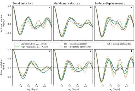
Figure 2.1: (a) The wind forcing (Fx, Fy) resembling trade winds and west- erlies over the domainD. (b) Wind profileγ. The points A, B will used for the analysis of autocorrelation (section3.6, Fig. 3.10 and 3.11).
2.1.2 Bottom friction
A quadratic drag of the following form is used for all model runs with bottom friction
b=−cD
h |u|u (2.6)
with cD being a dimensionless drag coefficient [Arbic & Scott, 2008]. In contrast to a linear drag, a quadratic drag was found to be more realistic.
It removes energy especially at the larger scales, leaving the smaller scales almost unaffacted. This is supported in this study (see section3.4).
The energetics of the bottom friction term are presented in section2.1.4.
In this study, we investigate a set of model runs containing bottom friction where we choose cD = 10−5 and another set of model runs without bottom friction (cD = 0) as described in Table2.1. The choice of cD is discussed in sectionA.2.6.
2.1.3 Lateral mixing of momentum
The viscosity is formulated as lateral mixing of momentum and represented by the termm. A general approachm0 of this family being
m0=∇ ·νS (2.7)
with the viscosity coefficient ν and a stress tensor S (sometimes also called viscous flux tensor [Eden, 2016]). With S = ∇u and a constant ν the equation 2.7reduces to
mL=ν∇2u (2.8)
with ∇2 = ∂x2 +∂y2 the two dimensional Laplace operator. However, as discussed byShchepetkin & O’Brien [1996] a more sophisticated alternative is found with the symmetric 2x2 stress tensorS defined by
S= ux−vy vx+uy
vx+uy −(ux−vy)
!
. (2.9)
Their harmonic lateral mixing of momentum termm2 is then formulated for the shallow water model as
m2 =νAh−1∇ ·hS. (2.10)
Note that for h being a constant equation 2.10 simplifies to equation 2.8.
Equation2.10can be extended to a biharmonic operator by applying it twice m=νBh−1∇ ·(hS(h−1∇ ·hS(u, v))). (2.11) where the stress tensor is regarded as a linear map, once evaluated with (u, v) and then with h−1∇ ·hS(u, v). Both viscosity coefficientsνA and νB are for simplicity taken as constants. Again, for a constant hequation 2.11reduces toνB∇4u, with∇4=∂x4+∂y4+ 2∂x2∂2y. Hence, for a barotropic system, where ηH it might be justified to linearize the viscous term by assuming h to be constant as inCooper & Zanna[2015]. However, here we keep the form of equation2.11to have a fully non-linear system. A higher order derivative implies the use of higher order boundary conditions: Applying the harmonic
operator twice yields additional boundary conditions as h∇2u+∇h· ux−vy
vx+uy
!
= 0, at x= 0 and x=Lx (2.12)
and
h∇2v+∇h· vx+uy
vy −ux
!
= 0, at y= 0 and y =Ly (2.13) For the case of a constanth this simplifies to a vanishing second derivative of the normal velocity component at the boundaries.
A biharmonic operator acts especially on the small scales, where waves are rapidly damped compared to the large scales, which remain mostly unaffected [Griffies & Hallberg,2000;Shchepetkin & O’Brien,1996]. To have an additional energy sink at the large scales, bottom friction from equation 2.6is used in combination with the biharmonic lateral mixing of momentum as presented here. For a discussion on the choice ofνB the reader is referred to sectionA.2.6. The choices for the different model runs are listed in Table 2.1.
2.1.4 Energetics in the shallow water model
In the following, energy sources/sinks and reservoirs in the shallow water system are discussed as they will be analyzed for all model runs in section 3.4.
The shallow water equations without forcing or dissipation (i.e. f =m= b= 0) obey a conservation of energy of the form
∂th12ρh(u2+v2) +12gρη2i= 0. (2.14) For a detailed derivation see Appendix A.3.1. The first term represents kinetic energy KE and the second (available) potential energy PE, both horizontally integrated byhi=RR
Ddxand vertically as are the momentum equations (2.1).
Energetics of wind forcing Once we consider wind forcingFxin equation 2.1a of the form as in equation 2.5
∂tu=...+ γ
ρh (2.15)
the energyhKE + PEi is not conserved
∂thKE + PEi=huγi (2.16) Once u and Fx are of the same sign, i.e. the flow follows the direction of the wind, the wind forcing term is a source of energy to the shallow water system. As we start the model runs from rest we can expect at least in the sense of a spatial and temporal average that the wind forcing is a source of energy to the shallow water system. This is discussed and supported in section 3.4.
Energetics of bottom friction Consider adding a drag term of the form in equation 2.6
∂tu=...−cD h
pu2+v2u (2.17)
that acts physically as bottom friction. The energy equation is then
∂thKE + PEi=−hρcD(u2+v2)32i ≤0. (2.18) which is with non-vanishing velocities an energy sink throughout the domain Dat every time step.
Energetics of lateral mixing A term of the form
∂tu=...+h−1∇ ·(νhS) (2.19) with viscosity coefficientν >0 and stress tensorSis added to the momentum equations. In fact, using a biharmonic lateral mixing of momentum this term should be negative to account for the correct sign of diffusion. Adaptation of the following for a biharmonic operator is straight forward. The energy equation is then
∂thKE + PEi=hρu·(∇ ·νhS)i. (2.20)
By evaluating
u·(∇ ·νhS) =∇ ·(νhS·u)− ∇u·νhS (2.21) and making use of the kinematic boundary condition the first term vanishes in the global integral as divergence of a flux and it follows that
∂thKE + PEi=−hρνh∇u·Si. (2.22) For the case ofS being the symmetric stress tensor defined in equation2.9, i.e. harmonic diffusion, lateral mixing is an energy sink as∂thKE + PEi=
−hρνh∇u·Si ≤0 not just spatially integrated but everywhere in the domain D(see section A.3.3for details). This is in contrast to biharmonic mixing operators (equation2.11), which are not sign-definite in that respect. As a result, the harmonic diffusion is always down-gradient, but the biharmonic diffusion can also lead to local power input in equation2.22 [Griffies,2004], but is in general also an energy sink.
Mean and eddy kinetic and potential energy Using Reynolds - de- composition in time allows to split every quanitityainto a time meanaand anomaliesa0 relative to aas
a=a+a0. (2.23)
However, in the shallow water system it is proposed to use thickness-weighted averaging [Aiki et al.,2016]
ba= ha
h (2.24)
The thickness-weighted average bais then used to compute the respective anomaliesa00
a00=a−ba (2.25)
Note that ha00 = 0. We can split the potential energy PE into mean potential energy (MPE) and eddy potential energy (EPE) with the thickness- unweighted decomposition
PE = 12gρ(η+η0)2 = 12gρη2+12gρη02 ≡MPE + EPE. (2.26)
For mean kinetic energy (MKE) and eddy kinetic energy (EKE) we use thickness-weighted decomposition on u andv
KE = 12ρh((bu+u00)2+ (bv+v00)2)
= 12ρ
h(ub2+bv2) +h(u002+v002) + 2uhub 00+ 2bvhv00
= 12ρh(bu2+bv2) +12ρh(u002+v002)
≡MKE + EKE (2.27)
2.2 Formulation of the energy budget-based backscat- ter parametrization
Following the ideas ofEden & Greatbatch[2008] for a mesoscale eddy closure, which are further developed inJansen & Held [2014];Jansenet al.[2015] we seek to find an energy equation for the unresolved scales, i.e. an equation for the sub-grid eddy kinetic energye, applied to the shallow water equations.
Similar toJansenet al. [2015] we formulate
∂te=−E˙diss+ ˙Eback+∇ ·νe∇e (2.28) with ˙Edissbeing the tendency representing the dissipation of the resolved flow that results from biharmonic viscosity. Adding this term to the prognostic equation of sub-grid EKEeis therefore a transfer of energy from the resolved to the unresolved flow. The term ˙Eback represents the tendency associated with the backscatter parametrization. It is the effect of energy transfer from the sub-grid EKE budget back onto the resolved flow and is realized with negative Laplacian viscosity. The last term of the right-hand side is a diffusion of sub-grid EKE.
For the shallow water model (equations 2.1) the local dissipation of eddy kinetic energy ˙Ediss associated with biharmonic viscosity (equation2.11) is in close relation to the energy equation2.22. Omitting the constant density ρ and the flux terms appearing in equations2.21 andA.83 yields
E˙diss=cdissνBh∇u·S∗ (2.29) with the biharmonic stress tensor S∗ = S(h−1∇ ·hS(u, v))) based on the symmetric stress tensor S from equation 2.9. E˙diss is negative where the
biharmonic lateral mixing of momentum removes energy from the resolved flow, which is usually the case. In contrast toJansenet al.[2015] we introduce a spatially and time-varying scalingcdiss which obeys
0≤cdiss(x, t)≤1 (2.30)
to allow only a fraction of the dissipated EKE to enter the sub-grid EKE budget. This is done for the following reasons:
(i) Having cdiss ≤ 1 yields an additional energy sink for the resolved flow, as the fraction 1−cdissis eventually dissipated and not subject to the recycling process of the backscatter parametrization. This might be as well desired for reasons of numerical stability. In case of vanishing bottom friction (b= 0), chosing cdiss= 1 would easily lead to an effective dissipation (taking both, biharmonic viscosity and the negative viscosity effect from backscatter, into account) that is too weak and below the allowed range to remain numerically stable.
(ii) In general, we can expect some flow dependence on the direction of energy cascades (upscale or downscale), which allows dissipation conditioned on properties of the locally resolved flow.
In order to match these, it is proposed to use cdiss= 1
(1 +R∗o)ndiss (2.31) with the deformation rate-based Rossby numberR∗o(see equation2.43), which is per definition non-negative. Hence, equation (2.31) obeys the condition of equation (2.30) for a positive constantndiss which remains subject to tuning.
Having a deformation rate-based scaling of dissipation viacdiss comes with the advantage that regions of strong shear, especially boundary currents that are subject to no-slip boundary conditions, experience a stronger dissipation than elsewhere. This avoids reinjecting an excess amount of energy via the backscatter terms locally where it may lead to spurious oscillations at the grid scale, that eventually lead to numerical instabilities. Physically speaking, we want to overcome the spurious energy dissipation at the grid scale for balanced flows, which tend to have a small Rossby number (which leads to cdissbeing close to 1) but retain the dissipative character for unbalanced flows
with large Rossby number [Rhines,1979;Zhaiet al.,2010]. This is motivated as geostrophic turbulence at small Rossby numbers tends to undergo an upscale cascade of energy, whereas large Rossby numbers are indicative of a downscale cascade where energy should indeed be dissipated [Br¨uggemann
& Eden,2015;Ferrari & Wunsch,2009;Molemakeret al.,2010].
Once the backscatter is realized with a negative Laplacian viscosity, that means the backscatter forcing terms in the shallow water equations (2.1) take the form
(ξx, ξy) =h−1∇ ·νbackhS (2.32) with a negative viscosity coefficient νback that is defined in equation 2.34. It follows that
E˙back =νbackh∇u·S (2.33) In contrast to Jansen et al. [2015], using a shallow water model, we consider the vertically integrated sub-grid EKE e of units m3s−2, which alters the scaling for νback slightly through dividing byh
νback =−cback∆x r
max(2e
h,0) (2.34)
so that νback retains its physical units as m2s−1. cback is an order O(1) non-dimensional constant, which we set as proposed in Jansenet al.[2015]
to be 0.4 and do not perform sensitivity experiments as general dependence was shown to be weak. Equation2.28can predict negative values ofe, hence using the maximum guarantees no backscatter in this case.
To summarize, we extend the shallow water equations with a prognostic equation for the vertically-integrated sub-grid EKEethat is
∂te=−cdissνBh∇u·S∗+νbackh∇u·S+∇ ·νe∇e. (2.35) From the perspective of the sub-grid EKE, the first term acts as a forcing, the second is a damping term asνbackis non-positive,h∇u·S≥0 (seeA.3.3) and monotonically decreasing with e; and the third is a diffusion term, and we set νe=νA(see section A.2.6).
Computational aspects For completeness, it is pointed out that the following simplifications for equations2.29 and 2.33hold:
E˙diss=cdissνBh(S11S∗11+S12S∗12), E˙back =νbackh S211+S212
(2.36) with a derivation in appendix A.3.2.
2.3 Reynolds and Rossby numbers
Definitons of the Reynolds and Rossby numbers directly calculated from the size of terms in the shallow water equations and adapted to the energy budget-based backscatter parametrization are presented.
Reynolds number The Reynolds number, defined as the ratio between advective and viscous terms, is traditionally estimated via scale analysis
Rce = O((u· ∇)u) O(ν∇2u) = U L
ν (2.37)
with some velocity scaleU, length scale Land viscosityν. It is also possible to directly compute the size of the advective and viscous term, i.e. replacing theO()-operation by the 2-norm of a vector and using the lateral mixing of momentum from equation (2.11)
Re = |(u· ∇)u|
|νBh−1∇ ·(hS(h−1∇ ·hS(u, v)))| (2.38) In the case of the backscatter parametrization, the effective Reynolds number R∗e also includes the backscatter term
R∗e = |(u· ∇)u|
|νBh−1∇ ·(hS(h−1∇ ·hS(u, v))) +νbackh−1∇ ·hS| (2.39) in order to account for the negative viscosity introduced by the backscatter parametrization. In fact, the terms in the denominator counteract each other:
The first tends to smooth gradients, whereas the second tends to steepen them. Using the backscatter parametrization we can expect thatR∗e > Re in an average sense.
Rossby number Via scale analysis the Rossby number Rco results from the ratio of advective terms and Coriolis terms as
Rco = O((u· ∇)u) O(fk×u) = U
f L (2.40)
with f being the Coriolis parameter and kthe unity vector in the vertical.
As in equation (2.38) the direct calculation for the Rossby numberRo yields Ro= |(u· ∇)u|
|fk×u| . (2.41)
It is also possible to base an estimation R∗o of the Rossby number on the deformation rate
|D|= q
(∂xu−∂yv)2+ (∂yu+∂xv)2 (2.42) which yields a large Rossby number R∗o in regions with strong shear flow
R∗o = |D|
f (2.43)
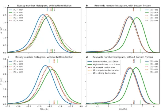
Histogram computation The direct Reynolds numbersRe and Rossby numbersRo will be investigated in terms of their histogram computed for all grid cells and all available time steps (without the spin-up phase, see section 2.6) at daily resolution. Hence, the histograms are computed from roughly 1.5·108 values in the low resolution case and 2.4·109 at high resolution.
The high resolution histograms are divided by a factor 16 to account for this and allow normalization onto the low resolution histograms. As Rossby and Reynolds numbers are approximately log-normally distributed the histogram is computed over their respective logarithms with a bin width of about 0.027 for Reynolds numbers and 0.018 for Rossby numbers. Also, a spatio-temporal mean Rossby and Reynolds number is computed, where the logarithm is applied afterwards for visualization purposes. For the model runs including backscatter, the effective Reynolds number R∗e is used instead to account for the backscatter term.
Rossby radius of deformation The Rossby radius of deformationLRo is defined via the shallow water phase speed for gravity wavescph=√
gH (see discussion around equation A.75 for further details) and the Coriolis
parameterf =f(y) as
LRo = cph
f . (2.44)
In the beta-plane approximation (equation 2.3), the Rossby radius is largest at the southern edge of the domain (y = 0) and smallest at the northern edge (y=Ly), it is therefore further distinguished between
LmaxRo = cph
f0−βL2y and LminRo = cph
f0+βL2y. (2.45)
2.4 Eddy kinetic energy spectrum
To have an objective analysis about the effect of sub-grid scale parametriza- tions, the eddy kinetic energy spectrum EKE(K) as a function of the total wavenumber K = √
k2+l2 is regarded. k is the zonal wavenumber (in x-direction),l the meridional wavenumber (iny-direction). Such a spectrum is especially sensitive to oscillations that may appear at the grid scale once dissipation is too weak. In this case, kinetic energy tends to pile up at the largest wave numbers, which results from the numerics and is physically undesired. The spectrum is defined as [Jansenet al.,2015]
EKE(K) = d dK
Z Z
k2+l2<K2
1 2
|ubt|2+|bvt|2
dkdl (2.46)
withubt,bvtbeing the spectral transforms of the two dimensional fields u, vfor a given time t. The overbar denotes a temporal mean. The EKE spectrum regarded here therefore describes the energy per wavenumber (regardless of the direction) averaged in spectral space over all available time steps.
2.5 Lagrangian trajectories
To calculate the trajectory of a Lagrangian float, we follow the idea that at a given timet the positionxp = (xp, yp) of that particle changes by passive advection of the flow field
dxp
dt =u(x=xp), dyp
dt =v(x=xp). (2.47)
Providing the initial position of the float xp(t= 0) we can solve equation 2.47 numerically with a given flow field (u, v). As the flow field is gridded on the native model grid, which in general does not correspond to the float positions, we interpolate bilinearly from the four surrounding grid points.
Taking the boundary conditions of the flow field into account, no float was observed to leave the domain D. However, due to a vanishing flow some floats remain at the boundary for a long time, which is thought of to be physically reasonable.
Discretizing the time derivative in equation2.47is done with a predictor- corrector method (also known as trapezoidal rule, [Butcher,2008]). With x0, y0 the intial positions at time t = t0 and x1, y1 the positions at time t=t0+δtthis is
x1 =x0+ δt
2(u0+u1), y1 =y0+δt
2(v0+v1) (2.48) where u0 = u(t = t0,x = x0) andv0 = v(t = t0,x =x0) and u1 = u(t = t0+δt,x=x∗1) andv1 =v(t=t0+δt,x=x∗1) with the initial guess positions x∗1 =x0+δtu0, y∗1 =y0+δtv0 (2.49) that are computed with Euler forward. The float trajectories are calculated offline, hence the time stepδt is 6 hours, as this is the smallest time step at which data from the numerical model is stored. We calculate trajectories from a total 100,000 floats, that where injected at 1000 random starting dates (after the spin-up phase) in groups of 100 floats. The trajectories are then calculated forward in time for one year. The results are presented in terms of accumulated float density, which accounts for all floats that have been at the respective location at some time within one year after release.
That means, accumulated float density is a histogram that counts all floats that have been in a given grid box (equal boxes of ∆x = ∆y = 15km are used), regardless of when they have been there within one year after release.
The zero-isoline of that histogram therefore denotes the line that no float was able to cross within one year. As release locations, we pick for every float a random position within a rectangle that spans fromx= 100km tox= 200km and from y = 100km to y = 1920km as marked in Fig. 3.12to place the floats close to the boundary within the subtropical gyre (a discussion is given in section3.7). If all floats were always far away from the boundary, then the
accumulated float density would be calculated from in total 146,000,000 float positions (100,000 floats at 1460 time steps that result from 6-hourly data for 365 days). However, as some floats stay for a long time close to the boundary, as discussed above, these are neglected from analysis by disregarding all float positions that are closer than 30km to the boundary. In practice, this means that 98% of all theoretical positions enter the analysis for the control runs and 94% for the model runs with backscatter.
2.6 Model runs and data sampling
For the list of model runs that are analysed in this study see Table 2.1.
List of model runs cD Nx ∆x νB ndiss tc
[km] [m4s−1] with bottom friction
Low resolution (LR) 10−5 1282 30 4.86·1011 - 1 High resolution (HR) 10−5 5122 7.5 7.59·109 - 50.2 LR + weak backscatter 10−5 1282 30 4.86·1011 12 1.39 LR + moderate backscatter 10−5 1282 30 4.86·1011 16 1.39 LR + strong backscatter 10−5 1282 30 4.86·1011 0 1.39 without bottom friction
Low resolution (LR) 0 1282 30 4.86·1011 - 0.93 High resolution (HR) 0 5122 7.5 7.59·109 - 46.7 LR + weak backscatter 0 1282 30 4.86·1011 12 1.30 LR + moderate backscatter 0 1282 30 4.86·1011 13 1.30 LR + strong backscatter 0 1282 30 4.86·1011 14 1.30 Table 2.1: List of model runs used in this study. The choice of the bottom friction coefficientcD and the biharmonic viscosityνB is discussed in section A.2.6. The tuning parameter for backscatterndiss appears in equation2.31.
The total number of grid cells is denoted withNx, the grid spacing with ∆x.
The computing timetc is given in relation to the computing time of the low resolution control run with bottom friction. Please note that the computing time is only roughly estimated and strongly dependent on the computing architecture.
For the analyses in this study, we use from every model run daily in-
stantaneous values on the native model grid of 30 year long integrations.
Spatial interpolation is only used in the computation of terms that involve prognostic variables from different grids (see sectionA.2.1). Only for the analysis of autocorrelation (section3.6) and Lagrangian trajectories (section 3.7) 6-hourly data is used for a better temporal resolution. A spin-up phase of 5 years, as discussed in section 3.2, is disregarded from all analysis except the timeseries in Fig. 3.2.
Model bias compared to the high resolution truth
This chapter presents a comparison of the two control runs that differ only by their spatial resolution and the viscosity coefficient that is altered accordingly.
The control runs do not include the backscatter parametrization, which will be introduced in chapter 4.
As we investigate the backscatter parametrization in an idealized ocean model set-up, there are no observations for reference. Hence, we regard the high resolution runs as the best approximation of the truth that is available, or shortly thetruth. In contrast, the low resolution run is regarded as the model, which claims to represent an ocean circulation with the same statistics as the high resolution truth. We therefore ignore implicitly, that also the high resolution truth is only an approximation towards a simulation with further increased resolution. From this perspective, this study only addresses the issue of a limited horizontal resolution in the range from eddy-permitting to eddy-resolving, which is however apparent in a wide range of ocean or climate models currently in use to simulate and understand the global climate system. Furthermore, based on the scale-invariance of the Navier-Stokes equations [Palmer,2012] we expect this issue also to project similiarly onto smaller scales and hence also to be of great importance in numerical weather prediction [Shutts, 2015]. Obviously, we cannot expect the low resolution model to simulate eddies that are barely resolved in the high resolution truth nor can we expect larger eddies to occur synchronously in both control runs.
However, we can demand the low resolution model to simulate statistically
the same ocean circulation in terms of mean state, energy, variability and a variety of other quantities. Section3.3 describes the model bias in terms of the climatological mean state. It follows a discussion of how the model differs with respect to energy compared to the truth in section 3.4. How much the physical regime, measured with Rossby and Reynolds numbers, disagrees between model and truth is presented in section 3.5. Section3.6 discusses model biases concerning time scales of the prognostic variables and is succeeded by an analysis of Lagrangian floats, how they spread differently in model and truth in section 3.7. A summary of model biases is given in section 3.8.
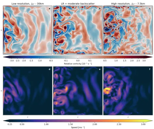
3.1 First view on the flow structure
Regarding snapshots of relative vorticity ζ=∂xv−∂yu and corresponding flow speeds|u|=√
u2+v2provides some insight into the dynamics simulated by both low resolution model and high resolution truth (Fig. 3.1). At high resolution, eddies of different sizes are apparent in most of the western part of the domain and especially also in the proximity of the southern and northern boundary (Fig. 3.1c). At low resolution, larger eddies are also simulated where the boundary current leaves the western boundary but they do not propagate as far into the domain (Fig. 3.1a). Also, the proximity of the northern and the southern boundary are rather eddy-free. The circulation dynamics are mostly dominated by westwards propagating Rossby waves in the eastern part of the domain and eddy-eddy interactions in the west [Marshall,1984]. The climatological double gyre circulation is not obvious from snapshots, only the western boundary current is predominant (Fig.
3.1d), when not masked locally by a rotational eddy flow. Especially at high resolution, instantaneous flow speeds may exceed 3 m/s, which is likely larger than maximum flow speeds observed in the global oceans. In the simulations regarded here, they usually occur between vortex dipoles (see Fig. 3.1c and f) and are therefore only of short durations. These findings do not change for runs with or without bottom friction.
Figure 3.1: Snapshot of (a,b,c) relative vorticity and (d,e,f) speed after 30 years of integration for model runs with bottom friction. The time steps of (a,d), (b,e) and (c,f) are associated, respectively. Positive vorticity is associated with clockwise rotation and vice versa. Please note the non-linear colormap for relative vorticity to highlight non-extreme structures.
3.2 Reaching statistical equilibrium
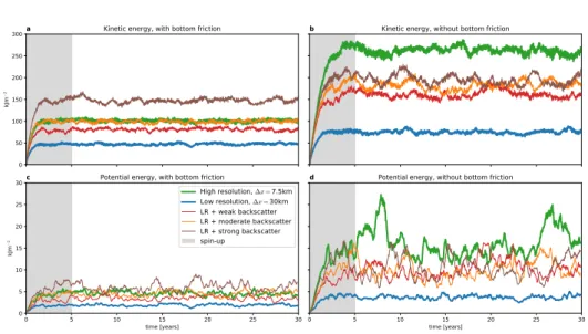
In order to investigate the climatological mean of both the low resolution model and the high resolution truth, a spin-up phase is disregarded, which is not representative for a statistical equilibrium that is reached afterwards. We choose kinetic and potential energy (see equation2.14) as a function of time to identify that a spin-up phase of 5 years is sufficient in that respect (Fig.
3.2). Furthermore, it is observed, that a higher resolution requires a longer spin-up phase. Simulations of very coarse resolution (∆x > 60km) reach their equilibrium state within weeks or months (not shown), presumably due to eddies not developing at such resolutions. It is likely that a higher level of kinetic and potential energy in the equilibrium state requires a longer spin-up
phase, such that also the bottom friction plays a crucial role: With bottom friction, the kinetic energy in the high resolution truth is approximately 100 kJm−2 (Fig. 3.2a), which is reached after 2 years, whereas switching off bottom friction yields almost three times higher levels of kinetic energy (Fig.
3.2b), that are only reached after 4 years of integration.
Due to the barotropic setting of the shallow water model (see section 2.1.1), the levels of potential energy are about one order of magnitude lower than those of kinetic energy. Using a gravitational acceleration ofg= 10m/s in contrast to a reduced gravity in a baroclinic setting, the restoring force of the free surface η is much stronger, disabling large displacements from the undisturbed layer thicknessH.
Comparing the energy levels between the low resolution model and the high resolution truth, we conclude that the model lacks energy in both its kinetic as well as its potential form by a factor of 2 to 3. Same relations between model and truth hold with and without bottom friction, respectively.
Furthermore, bottom friction reduces the energy levels again by a factor of 2 to 3. Increased energy levels are also observed to conincide with enhanced long-term variability on multi-annual time scales, although seasons are absent from the shallow water model due to a time-constant wind forcing: In the high resolution truth without bottom friction, the level of potential energy is almost doubled from year 5 to 10 and from year 25 to 30 compared to other years (Fig. 3.2d). This kind of long-term variability is absent from the low resolution model, presumably due to lower levels of energy. However, this does not necessarily follow from altered ocean dynamics but can already be explained by integrating white noise in time with larger variance, which yields a larger variability simultaneously on all temporal scales.
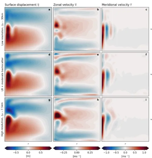
3.3 Climatological mean state
Both, the low resolution model and the high resolution truth simulate in the time mean a double gyre circulation with (Fig. 3.3) and without bottom friction (Fig. 3.4) with a strong boundary current (e.g. the Gulf stream or Kuroshio in analogy to the real ocean) at speeds of about 1 m/s (Fig.
3.3c and i, and Fig. 3.4c and i). The southern (northern) gyre is referred to as sub-tropical (sub-polar) gyre. The low resolution model shows a weak inter-gyre gyre in the north-east corner, that reaches half-way to the west
0 50 100 150 200 250 300
kJm−2
Kinetic energy, with bottom friction
a b Kinetic energy, without bottom friction
0 5 10 15 20 25 30
time [years]
0 5 10 15 20 25 30
kJm−2
Potential energy, with bottom friction c
High resolution, ∆x=7.5km Low resolution, ∆x=30km LR + weak backscatter LR + moderate backscatter LR + strong backscatter spin-up
0 5 10 15 20 25 30
time [years]
Potential energy, without bottom friction d
Figure 3.2: (a) Spatially integrated kinetic energy for 30-year long integrations of model runs as described in Table2.1with bottom friction. (b) as (a) but for model runs without bottom friction. (c) Potential energy for model runs with bottom friction, (d) as (c) but without bottom friction. Time series of potential energy are low-pass filtered with a running mean of window size of three months for clarity. The spin-up phase of 5 years is omitted for all analyses. Kinetic and potential energy is defined in equation2.14.
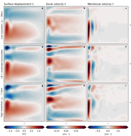
(Fig. 3.3a and Fig. 3.4a). This inter-gyre gyre is more prolonged in the high resolution truth (Fig. 3.3g), especially without bottom friction (Fig. 3.4g).
Having no bottom friction, a standing eddy develops in the north-west corner (Fig. 3.4g,h and i) that turns out to be much weaker without bottom friction (Fig. 3.3g,h and i) but is absent from all low resolution runs. Defining the across-basin current (e.g. the North Atlantic current in analogy to the real ocean) path as the mostly zonal zero-isoline of the surface displacement that reaches from the western boundary far into the east in our model runs, we observe at least some depedence on the resolution: At higher resolution and also higher energy levels (i.e. comparing with and without bottom friction) the across-basin current path is less undulated. This leads to the conclusion that any temperature bias in current global ocean or climate models [Flato et al.,2013;Large & Danabasoglu, 2006] may already result from altered
eddy dynamics due to a limited resolution.
Figure 3.3: Climatological mean of the prognostic variables u, v, η for the model runs with bottom friction (see Table 2.1). The mean is calculated over 25 years, disregarding a spin-up of 5 years (see Fig. 3.2).
3.4 Energetics
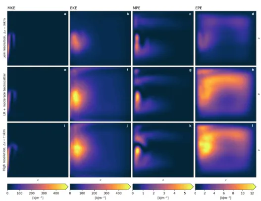
As we have already seen in the previous section and especially in Fig. 3.2, the low resolution model simulates considerably lower energy levels, both kinetic and potential, compared to the high resolution truth. This section aims to understand this issue by regarding different energy reservoirs, namely mean kinetic energy (MKE, see equation2.27), eddy kinetic energy (EKE), mean potential energy (MPE, see equation2.26) and eddy potential energy (EPE) as well as the eddy kinetic energy spectrum and energy sources and
sinks due to different terms in the energy equation (section2.1.4).
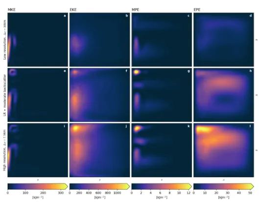
Figure 3.4: Same as Fig. 3.3 but for the model runs without bottom friction (see Table 2.1). Please note the different scaling of the color-shading.
Following the Reynolds decomposition into mean and anomalies (equation 2.23), we first point out that splitting kinetic and potential energy into its respective mean and eddy contribution refers to the time domain. In that respect, an eddy is a temporal anomaly and is not directly related to a spatially coherent structure with certain dynamics. Nevertheless, turbulence theory claims some similarities in the space and time domain, such that conclusions in one have some validity in the other [Palmer,2012]. Keeping this in mind we carefully draw conclusions in the following analysis.
Both, the low resolution model and high resolution truth simulate high levels of MKE within the western boundary current, reaching into a weak
Figure 3.5: Climatological mean of mean kinetic energy (MKE), eddy kinetic energy (EKE), mean potential energy (MPE) and eddy potential energy (EPE) which are thickness-weighted as defined in equations2.26and 2.27.
Shown are the model runs with bottom friction.
recirculation branch within the across-basin current (Fig. 3.5a and i). The same holds with and without bottom friction at comparable amplitude (Fig.
3.6a and i). This supports that only this part of the basin-wide circulation is a temporally prevailing current, whereas the flow in most other parts of the domain are either eddy-driven or caused by Rossby-waves but then negligible in strength. Consequently, there is a comparably enormous reservoir of EKE in the central western part of the domain, which is a factor of 2 to 3 larger in the high resolution truth compared to the low resolution model (Fig. 3.5b and j, and also without bottom friction in Fig. 3.6b and j). We therefore conclude that the lack of energy in the low resolution model compared to the high resolution truth is mostly due to lower levels of EKE and less so in terms of MKE. Similar conclusions hold for potential energy: MPE (Fig.
3.5c and k) follows mainly the climatogical mean of the surface displacement (Fig. 3.3a and i) with comparable amplitude but slightly different structure
Figure 3.6: Same as Fig. 3.5 but for the model runs without bottom friction (see Table 2.1). Please note the different scaling of the color-shading.
due to the differences in the climatological mean circulation. In contrast, the EPE reservoir (Fig. 3.5d) is much larger than MPE (Fig. 3.5c) and spans throughout the northern part of the domain and especially pronounced in the central western part, where also EKE is found to be largest. Although similar in structure, the EPE reservoir is a factor of 2 to 3 larger in the high resolution truth (Fig. 3.5l) compared to the low resolution model (Fig.
3.5d).
This points towards the same conclusion: The low resolution especially lacks energy in the eddy contribution to kinetic and potential energy compared to the high resolution truth, which seems to be independent of bottom friction.
In order to understand the differences in eddy energy that come with different resolution we analyse the energy sources and sinks of the different terms in the shallow water equations (eq. 2.1). Without wind forcing, lateral mixing of momentum and bottom friction the shallow water equations obey conservation of energy, so that starting from rest these terms must explicitly account for sources and sinks of kinetic and potential energy to explain the
initial accumulation of energy in the spin-up phase as well as the leveling off to a statistical equilibrium afterwards. Regarding the climatological mean, where in the time-mean sense the amount of energy in the system is steady (Fig. 3.2), it is pointed out that all sources and sinks, once spatially integrated, must balance out. A local imbalance is compensated by the flow being able to propagate energy throughout the domain.
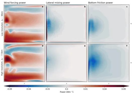
Wind forcing is found to be an energy source in large areas throughout the basin and an energy sink in others in both low resolution model and high resolution truth (Fig. 3.7a and d), which depends on the direction of the mean flow compared to the direction of the wind (see equation 2.16). Spatially integrated wind forcing is the only energy source to the shallow water system in the physical setting regarded here, and additionally largely independent of the resolution. The power due to the lateral mixing of momentum term altering the energy budget (Fig. 3.7b and e) reveals an energy sink in the eddy-dominated central western part of the domain, which is strong in the low resolution control but much weaker in the high resolution truth. The lateral mixing of momentum in connection with no-slip boundary conditions also removes lots of energy from the boundary. Due to the operator being biharmonic and therefore not sign-definite (see section 2.1.4) some of the energy that is removed right at the boundary is partly reinjected a grid cell or two farther away. Bottom friction removes energy largely from the western boundary current and the across-basin current being its extension, as flow speeds are fastest here. The pattern therefore resembles that of MKE (Fig.
3.5a and i). The energy removal due to bottom friction is slightly larger in the high resolution truth than in the low resolution model.
It is hence concluded that the effect of the lateral mixing on the energy budget is resolution dependent: Having a larger viscosity coefficient at coarser resolution yields a larger dissipation, that is usually understood as spuriously high compared to the real ocean, but necessary for numerical stability [Griffies
& Hallberg,2000].
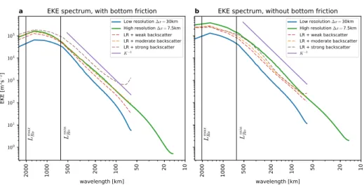
Although the biharmonic lateral mixing of momentum is known to remove energy at the grid scale [Jansen & Held, 2014; Jansenet al., 2015], it affects all spatial scales as seen in the EKE spectrum (Fig. 3.8). Most EKE is concentrated on spatial scales of the Rossby deformation radius with a power law decrease towards the grid scale being close to K−3, pointing to a clearly developed turbulence cascade over a wide range of scales. Only with bottom
Figure 3.7: Climatological mean of energy sources and sinks due to wind forcing, lateral mixing of momentum and bottom friction for the two control runs without backscatter parametrization: (a,b,c) low resolution and (d,e,f) high resolution (see Table 2.1) with bottom friction. The power of the different terms is given in equations 2.16, 2.22 and 2.18. Positive values indicate an energy source and negative an energy sink to the system. Please note the non-linear colormap for visualization purposes.
friction the high resolution truth shows a slightly less steep descent, which is supported by other studies [Capetet al.,2008]. Bottom friction is found to remove energy by a factor of about three from the largest scales, leaving the smaller scales mostly unaffected (compare Fig. 3.8a with b). This relates to removing energy from the largest eddies, which are responsible for the fastest flow speeds (Fig. 3.1d and f). From the perspective of the EKE spectrum it is concluded that for a successful parametrization it is necessary to either decrease the dissipation in the low resolution model or to reinject energy, such that spectral fluxes spread it across scales, in order to increase the EKE level.
2000 1000 500 200 100 50 20 10 wavelength [km]
100 101 102 103 104 105
EKE [m3s−2] Lmax Ro Lmin Ro
EKE spectrum, with bottom friction a
Low resolution ∆x=30km High resolution ∆x=7.5km LR + weak backscatter LR + moderate backscatter LR + strong backscatter K−3
2000 1000 500 200 100 50 20 10
wavelength [km]
Lmax Ro LminRo
EKE spectrum, without bottom friction b
Low resolution ∆x=30km High resolution ∆x=7.5km LR + weak backscatter LR + moderate backscatter LR + strong backscatter K−3
Figure 3.8: (a) Eddy kinetic energy spectrum for the model runs with bottom friction and (b) without (see Table 2.1). A theoretical spectrum of K−3 is given for comparison. The spectral energy is logarithmically plotted against horizontal wavenumber K but for readability relabelled with the corresponding wavelength. The Rossby radii of deformationLmaxR
o , LminR
o
(equation2.45) are given for orientation.
3.5 Physical regime
To understand the difference between the low resolution model and the high resolution truth we furthermore investigate the physical regime in terms of Rossby and Reynolds numbers of these simulations. Both, Rossby and Reynolds numbers are directly calculated from the size of the terms in the shallow water equations2.1for every grid cell and every available time step as described in section 2.3. Distributions of Rossby and Reynolds numbers are shifted towards smaller values in the low resolution model compared to the high resolution truth (Fig. 3.9). Also bottom friction decreases the Rossby numbers, but has almost negligible effect on the Reynolds numbers. Rossby numbers follow approximately a log-normal distribution, as they are visibly normal distributed when plotted logarithmically on the abcissa. Similar for Reynolds numbers, whose distribution is a bit more skewed, with a fatter tail at low values (Fig. 3.9b and d). Low resolution model and high resolution truth both simulate a wide range of Rossby and Reynolds numbers: The 2.5th and 97.5th percentile span roughly two orders of magnitude for Rossby numbers and three to four orders of magnitude for Reynolds numbers.