THE ARCTIC

(1)

THE ARCTIC

CLOUD PUZZLE

Using ACLOUD/PASCAL Multiplatform Observations to Unravel the Role of Clouds and Aerosol Particles in Arctic Amplification

Employing two research aircraft, one icebreaking research vessel, an ice floe camp including an instrumented tethered balloon, and a permanent ground-based measurement station at Spitsbergen, a consortium of polar scientists combined observa- tional forces in a field campaign of unprecedented complexity to uncover the secrets of clouds and their role in Arctic amplification.

Manfred Wendisch, andreas Macke, andré ehrlich, ch r i s to f lü p k e s, Ma r i o Mec h, dM itry ch ec h i n, klaus dethloff, carola Barrientos Velasco, heiko

BozeM, Marlen Brückner, hans-christian cleMen, susanne creWell, toBias donth, regis dupuy, kerstin

eBell, ulrike egerer, ronny engelMann, christa engler, oliVer eppers, Martin gehrMann, Xianda gong, Matthias

gottschalk, christophe gourBeyre, hannes griesche, Jörg hartMann, Markus hartMann, Bernd heinold, andreas herBer, hartMut herrMann, georg heygster, peter hoor, soheila JafariseraJehlou, eVelyn Jäkel, eMMa

JärVinen, oliVier Jourdan, udo kästner, siMonas kecorius, erlend M. knudsen, franziska köllner, Jan kretzschMar, luca lelli, delphine leroy, Marion Maturilli, linlu Mei, stephan Mertes, guillauMe Mioche, roland neuBer, Marcel nicolaus, tatiana noMokonoVa, Justus notholt, Mathias palM, Manuela Van pinXteren, Johannes Quaas, philipp richter, elena ruiz-donoso, Michael schäfer, katJa schMieder, Martin schnaiter, Johannes schneider, alfons schWarzenBöck, patric seifert, MattheW d. shupe, holger sieBert, gunnar spreen, Johannes stapf, frank

stratMann, teresa Vogl, andré Welti, heike WeX, alfred

Wiedensohler, Marco zanatta, and seBastian zeppenfeld

C

urrently, we are witnessing drastic climate changes in the Arctic that are unprecedented in the history of mankind (Jeffries et al. 2013). Within about the last 40 years, the Arctic sea ice extent has decreased dramatically (Stroeve et al. 2012); in particular, the September minimum of sea ice extent dropped by almost two-thirds. The maximum extent of winter sea ce has shrunk significantly as well (Onarheim et al. 2018). In March 2017 the Arctic maximum sea ice extent decreased to its smallest value ever recorded (Richter-Menge et al. 2017). Also, the thickness of the sea ice has declined. Multiyear thick sea ice made up only 21% of the sea ice cover in 2017; in 1985 this value was about 45% (Richter-Menge et al. 2017). Because thin ice melts faster than thick ice, the thin ice gets thinner and a positive feedback occurs.

Concurrently, the Arctic near-surface temperature considerably increased within the last three to four decades, and it continues to rise at double the rate of global average values—a phenomenon commonly called Arctic amplification (Serreze and Barry 2011). In 2017 the mean Arctic near-surface air temperature over land exceeded the 1981–2010 average by 1.6°C, which is (after 2016) the second-highest average ever 

Overflight over the R/V Polarstern with the research aircraft Polar 5 over the Marginal Ice Zone (MIZ) north of Svalbard

(2)

recorded (Richter-Menge et al. 2017). As a result the melting season starts earlier and the freeze-up begins later. For example, the freeze-up in 2016 in the Barents and Kara Seas was among the latest ever reported. It is evident that the winter season is becoming particularly impacted by Arctic warming.

Unfortunately, we neither fully comprehend these striking climate changes in the Arctic nor understand why they happen so fast. As a result we are unable to reliably predict how the Arctic climate will evolve in the future (Screen et al. 2018). Even worse, we cannot evaluate the substantial consequences a warming and thawing Arctic might have for midlatitude weather (Cohen et al. 2014; Walsh 2014; Cohen et al. 2018).

Therefore, several international efforts are underway to improve model projections of the Arctic climate, such as the Polar Prediction Project and the Year of Polar Prediction (Jung et al. 2016). However, models alone will not resolve the Arctic climate issue. They often use simple parameterizations, which need to be verified, tested, and improved by measurements. The required observations are still sparsely distributed across the Arctic. As a consequence further data should be collected in well-planned and dedicated campaigns to document and understand the Arctic climate changes. Such observations are costly and require tremendous organizational efforts, including the logistics (aircraft, icebreaker, etc.), which are challenging in the harsh environmental conditions in the Arctic.

Advances in land-based observations [e.g., obtained by the work of the International Arctic Systems for Observing the Atmosphere (IASOA)] help to provide important insights into the changing Arctic climate system (Uttal et al. 2016). However, targeted observations that focus on special Arctic phenomena [such as mixed-phase clouds, stable atmospheric boundary layer (ABL), polar day and night, high surface reflectivity] are needed to clarify key ele- ments that are thought to contribute to the Arctic amplification phenomenon (Wendisch et al. 2017).

This should also include relevant processes such as airmass transformations during meridional transport (Pithan et al. 2018). For this purpose it is essential to organize concerted observational campaigns looking at certain aspects of the changing Arctic system, such as the Multidisciplinary Drifting Observatory for the Study of Arctic Climate (MOSAiC) campaign, which is planned for 2019/20 (www.mosaic-expedition.org).

Furthermore, it is crucial to implement sustained research programs, such as the German Arctic Amplification: Climate Relevant Atmospheric and Surface Processes, and Feedback Mechanisms [(AC)³; www.ac3-tr.de/] project, that orchestrate observations and modeling efforts (Wendisch et al. 2017).

Because the current changes of the Arctic climate system happen so fast, it is likely that atmospheric processes play a major role. Therefore, a large number of previous airborne and ship-based campaigns were particularly focused on atmospheric and surface

AFFILIATIONS: Wendisch, ehrlich, Brückner, donth, engler, gottschalk, Jäkel, kretzschMar, Quaas, ruiz-donoso, schäfer,

and stapf—Leipziger Institut für Meteorologie, Universität Leipzig, Leipzig, Germany; Macke, Barrientos Velasco, egerer, engelMann, gong, griesche, M. hartMann, heinold, herrMann, kästner, kecorius, Mertes, Van pinXteren, schMieder, seifert, sieBert, stratMann, Vogl, Welti, WeX, Wiedensohler, and zeppenfeld—Leibniz-Institut für Troposphärenforschung, Leipzig, Germany; lüpkes, chechin, deth-

loff, gehrMann, J. hartMann, herBer, Maturilli, neuBer, nicolaus,

and zanatta—Alfred-Wegener-Institut, Helmholtz-Zentrum für Polar- und Meeresforschung (AWI), Bremerhaven, Germany; Mech, creWell, eBell, knudsen, and noMokonoVa—Institut für Geo- physik und Meteorologie, Universität zu Köln, Cologne, Germany;

BozeMand hoor—Institut für Physik der Atmosphäre, Johannes Gutenberg-Universität, Mainz, Germany; eppers—Institut für Physik der Atmosphäre, Johannes Gutenberg-Universität, and Particle Chemistry Department, Max Planck Institute for Chemistry, Mainz, Germany; cleMen, köllner, and schneider—Particle Chemistry Department, Max Planck Institute for Chemistry, Mainz, Germany;

heygster, JafariseraJehlou, lelli, Mei, notholt, palM, richter, and

spreen—Institut für Umweltphysik, Universität Bremen, Bremen, Germany; JärVinenand schnaiter— Institut für Meteorologie und

Klimaforschung, Karlsruher Institut für Technologie, Karlsruhe, Ger- many; dupuy, gourBeyre, Jourdan, leroy, Mioche, and schWarzen-

Böck—Laboratoire de Météorologie Physique, Université Clermont Auvergne/OPGC/CNRS, UMR 6016, Clermont-Ferrand, France;

shupe—Earth System Research Laboratory, National Oceanic and Atmospheric Administration, and Cooperative Institute for Research in the Environmental Sciences, University of Colorado Boulder, Boulder, Colorado

CORRESPONDING AUTHOR: Manfred Wendisch, m.wendisch@uni-leipzig.de

The abstract for this article can be found in this issue, following the table of contents.

DOI:10.1175/BAMS-D-18-0072.1

A supplement to this article is available online (10.1175/BAMS-D-18-0072.

In final form 30 October 2018

For information regarding reuse of this content and general copyright information, consult the AMS Copyright Policy.

This article is licensed under a Creative Commons Attribution 4.0 license.

842 | MAY 2019

(3)

processes, partly neglecting the long-term effects of the slowly changing ocean. Several examples of these previous efforts are discussed in the sidebar “Previous airborne and ship-based campaigns in the Arctic,”

which is summarized in Table 1 (including respective references), to provide context for new observations.

These past campaigns generally highlighted the important role that clouds can—and do— play in that changing system and in the manifestation of Arctic amplification. However, there is still a basic lack of understanding of the interplay between aerosol particles, clouds, and surface properties, as well as turbulent and radiative fluxes with dynamical processes, that currently prevents accurately simulating clouds in the Arctic climate system. The sidebar “The Arctic Cloud Puzzle” introduces the puzzling problems related to Arctic clouds in more detail.

To enhance the existing knowledge on the role of Arctic clouds and aerosol particles in the Arctic climate system, and thereby to help to further solve this Arctic cloud puzzle, two concerted field studies have been performed: Arctic Cloud

Observations Using Airborne Measurements during Polar Day (ACLOUD) and Physical Feedbacks of Arctic Boundary Layer, Sea Ice, Cloud and Aerosol (PASCAL). The jointly planned and organized observations took place around Svalbard, Norway, in May and June 2017. ACLOUD consisted of airborne observations by two research aircraft, Polar 5 and Polar 6 (Wesche et al. 2016). PASCAL involved measurements from the Research Vessel (R/V) Polarstern (Knust 2017) and an ice floe camp [including the Balloon-bornE moduLar Utility for profilinG the lower Atmosphere (BELUGA) tethered balloon]. A detailed summary of the measurements performed during PASCAL can be found in Macke and Flores (2018). Additionally, measurements from the permanent joint research base operated by Alfred Wegener Institute (AWI) and the French Polar Institute Paul- Émile Victor (IPEV; AWIPEV) at Ny-Ålesund (Sval- bard) were involved (Neuber 2006). The ACLOUD and PASCAL campaigns are unique in that both were tightly coordinated under the collaborative (AC)³ pro- gram (Wendisch et al. 2017), funded by the German

PREVIOUS AIRBORNE AND SHIP-BASED CAMPAIGNS IN THE ARCTIC

M

IZEX West (1983) and MIZEX East (1984) were aimed at understanding the effects of the marginal ice zone (MIZ) with a focus on air–ice–sea exchange processes. Both projects were large international campaigns that were conducted with several ships and aircraft. REFLEX I, II, and III focused on i) the influence of the MIZ on transfer coefficients, ii) the cloud impact on radiation flux densities as well as the parameterizations of the surface albedo as a function of sea ice fraction and solar zenith angle, and iii) the investigation of cold-air outbreaks. IAOE focused on the potential climatic control of dimethyl sulfide (DMS). The main goal of the comprehensive SHEBA campaign was to study the surface heat and energy budget of the sea ice–covered ocean, based on continuous and mostly shipborne measurements over one year at a station drifting in the Beaufort Gyre. ARTIST pursued goals similar to REFLEX but with a dedicated focus on airborne turbulence measurements in cold-air outbreaks. The ASTAR I, II, and III series of airborne campaigns investigated aerosol–cloud interactions and the resulting modifications

of radiative properties of clouds. Fram Strait cyclones and their impact on sea ice development were studied during the FRAMZY series of observations carried out with buoys and aircraft. The AOE campaign investigated summer meteorological conditions and clouds.

M-PACE merged the observations of two stationary ground-based sites and two aircraft to study physical processes in Arctic mixed-phase clouds. ISDAC investigated aerosol–cloud interactions in the ABL. Two POLARCAT campaigns operated from northern Sweden and Kangerlussuaq (Greenland) during the International Polar Year (2008).

ARCPAC was an airborne campaign coordinated with POLARCAT; it was closely collocated with remote sensing and in situ observations from the ground site of Barrow, Alaska (now known as Utqiag·vik). ASCOS also focused on late summer cloud–aerosol interactions in the central Arctic. MELTEX concentrated on the importance of melt ponds on surface albedo during the initial stage of sea ice melt. IceBridge uses airborne instruments to obtain maps of ice sheets, ice shelves, and sea ice of Arctic and Antarctic areas once

a year. ARCTAS studied the influx of midlatitude pollution, boreal forest fires, aerosol radiative forcing, and chemical processes. A series of airborne research campaigns using the Polar 5 and Polar 6 research aircraft was conducted out of Svalbard and Inuvik (northern Canada) during SORPIC, VERDI, and RACEPAC. These measurements investigated aerosol–cloud–radiation interactions. ACCACIA was conducted to measure aerosol and cloud effects on the Arctic surface energy balance and climate. STABLE mainly investigated the impact of leads on the ABL and cold-air outbreaks with a focus on the flow between the inner Arctic and the marginal sea ice zone. NETCARE focused on carbonaceous aerosol, ice cloud formation and impact, and ocean–atmosphere interactions. ARISE collected airborne data on clouds, atmospheric radiation, and sea ice properties between the sea ice minimum in September and the beginning of refreezing in late autumn. ACSE looked at Arctic clouds in summer. N-ICE studied how the rapid shift to a younger and thinner sea ice re- gime in the Arctic affects energy fluxes and sea ice dynamics.

(4)

T^able 1. Examples of major campaigns focused on atmospheric and surface processes performed in the Arctic;

the list is not complete.

Full name Acronym Year Area Airborne

Ship

based Selected references Marginal Ice Zone

Experiment West

MIZEX West 1983 Bering Sea   Cavalieri et al. (1983)

Marginal Ice Zone Experiment East

MIZEX East 1984 Greenland Sea   MIZEX Group (1986)

Radiation and Energy Flux Experiments I, II, III

REFLEX I, II, III

1991, 1993, 1995

Fram Strait   Hartmann et al. (1992, 1994)

Kottmeier et al. (1994) Freese and Kottmeier (1998) International Arctic Ocean

Expedition

IAOE 1991 Central

Arctic

 Leck et al. (1996) Surface Heat Budget of the

Arctic Ocean

SHEBA 1997/98 Beaufort Sea   Curry et al. (2000)

Uttal et al. (2002) Perovich et al. (2003) Shupe et al. (2006) Verlinde et al. (2007) Arctic Radiation and

Turbulence Interaction Study

ARTIST 1998 Fram Strait  Hartmann et al. (1999)

Gryanik and Hartmann (2002) Gryanik et al. (2005) Arctic Study of Aerosol,

Clouds and Radiation I, II, III

ASTAR I, II, III

2000, 2004, 2007

Svalbard  Special issue of Atmos. Chem.

Phys.^a Fram Strait Cyclones and

Their Impact on Sea Ice

FRAMZY 1999, 2002, 2007, 2008,

2009

Fram Strait  Brümmer et al. (2008)

Collection of papers^b Arctic Ocean Experiment AOE 1996, 2001 Central

Arctic Ocean

 Tjernström et al. (2004) Mixed-Phase Arctic Cloud

Experiment

M-PACE 2004 Alaska  Verlinde et al. (2007)

Indirect and Semidirect Aerosol Campaign

ISDAC 2008 Alaska  McFarquhar et al. 2011)

Polar Study Using Aircraft, Remote Sensing, Surface Measurements and Models of Climate, Chemistry, Aerosols, and Transport

POLARCAT 2008 Sweden,

Greenland

  Delanoe et al. (2013)

Law et al. (2014)

Aerosol, Radiation, and Cloud Processes Affecting Arctic Climate

ARCPAC 2008 Barrow,

Alaskan Arctic

 Brock et al. (2011)

Arctic Summer Cloud Ocean Study

ASCOS 2008 Central

Arctic

 Tjernström et al. (2014) Shupe et al. (2013) Sedlar and Shupe 2014) Melt Ponds on Energy and

Momentum Fluxes between Atmosphere and Ocean

MELTEX 2008 Beaufort Sea  Rösel and Kaleschke (2012)

Arctic Research of the Composition of the Troposphere from Aircraft and Satellites

ARCTAS IceBridge

2008 2009–16

Alaska Western Arctic Ocean



Jacob et al. (2010) Kurtz et al. (2013)

Solar Radiation and Phase Discrimination of Arctic Clouds

SORPIC 2010 Svalbard  Bierwirth et al. (2013)

Continued on next page

844 | MAY 2019

(5)

Research Foundation [Deutsche Forschungsgemein- schaft (DFG)]. From the beginning, modeling needs and perspectives guided the design and planned analyses from a unique set of closely collocated airborne (aircraft, tethered balloon), ground-based (ship, ground station), and satellite observations.

The general strategy of the measurements as well as the meteorological, sea ice, and cloud conditions during ACLOUD/PASCAL are introduced in the following section. The measured and retrieved quantities collected during the campaigns are briefly explained in the “Measured quantities and major instrumentation” section, while most of the details, in particular with respect to the instruments, are given in a sepa- rate online supplement (https://doi.org/10.1175/BAMS -D-18-0072.2). Then two illustrative examples of collocated measurements are presented to demonstrate

the potential of the combined datasets. The major part of the paper (“Four pieces of the Arctic cloud puzzle”) discusses selected measurement cases to investigate four pieces of the Arctic cloud puzzle.

Finally, in the “Summary and open questions” section, a summary of the paper is given, including questions to be answered in the forthcoming data analyses of the ACLOUD and PASCAL campaigns and future research activities.

INTRODUCTION OF AC LOU D AN D PASCAL CAMPAIGNS. Complementary cloud observations. The general measurement approach of ACLOUD and PASCAL is depicted in Fig. 1.

One aircraft (Polar 5) was used as a remote sensing platform observing the clouds from above, while the other aircraft (Polar 6) went into and below the T^able 1. Continued.

Full name Acronym Year Area Airborne Ship

based Selected references Vertical Distribution of Ice

in Arctic Clouds

VERDI 2012 Inuvik  Joint special issue: Atmos.

Meas. Tech.

Atmos. Chem. Phys.^c Aerosol–Cloud Coupling and

Climate Interactions in the Arctic

ACCACIA 2013 Svalbard  Lloyd et al. (2015); Jones et

al. (2018) Spring Time Atmospheric

Boundary Layer Experiment

STABLE 2013 Fram Strait  Tetzlaff et al. (2014, 2015)

Network on Climate and Aerosols: Addressing Key Uncertainties in Remote Canadian Environments

NETCARE 2013, 2014, 2015

Central Arctic

 Collection of papers^d

Radiation–Aerosol–Cloud Experiment in the Arctic Circle

RACEPAC 2014 Inuvik  Costa et al. (2017)

Arctic Radiation IceBridge Sea and Ice Experiment

ARISE 2014 Alaska  Smith et al. (2017)

Arctic Clouds in Summer Experiment

ACSE 2014 Eastern

Arctic Ocean

 Sotiropoulou et al. (2016) Along

Russian Coast

 Tjernström et al. (2015) Norwegian Young Sea Ice

Cruise

N-ICE 2015 North of

Svalbard

 Special section in J. Geophys.

Res. Oceans^e Aerosol–Arctic Cloud

Observations Using Airborne Measurements during Polar Day and Physical Feedbacks of Arctic Boundary Layer, Sea Ice, Cloud

ACLOUD/

PASCAL

2017 Svalbard   This paper

a Please see www.atmos-chem-phys.net/special_issue151.html.

b Please see https://cera-www.dkrz.de/WDCC/ui/cerasearch/q?query=FRAMZY&page=0&rows=15.

c Please see www.atmos-meas-tech.net/special_issue10_362.html.

d Please see www.atmos-chem-phys.net/special_issue835.html.

e Please see http://agupubs.onlinelibrary.wiley.com/hub/issue/10.1002/(ISSN)2169-9291.NICE1/.

(6)

clouds. Ground-based observations of the whole vertical column of cloud and aerosol particles were performed at the R/V Polarstern (ship and ice floe camp) and at Ny-Ålesund, mainly using remote sensing techniques. This was complemented by ABL (in situ) measurements at both sites. For example, the BELUGA tethered balloon was operated from the ice floe camp; it served as a linkage between the aircraft and the ground-based observations. In ad- dition, aircraft underflights of the A-Train satellites (Stephens et al. 2018) provided context for the two campaigns. These satellite data are not discussed in this paper; they will be analyzed in forthcoming publications on ACLOUD/PASCAL. The time period of the ACLOUD and PASCAL campaigns extended from 23 May to 26 June 2017, defined by the full length of aircraft activities. The ice floe camp was set up between 5 and 14 June 2017.

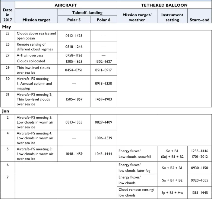
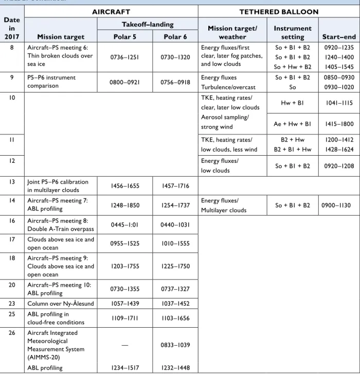
Each aircraft completed 19 measurement flights (165 flight hours in total), of which 16 were coordinated flights between the two aircraft. The horizontal flight paths of the aircraft and the track of the R/V Polarstern are shown in Fig. 2. Table 2 summarizes all aircraft and tethered balloon flights. Ten coordinated aircraft flights were performed above the R/V Polarstern, while 13 occurred over the Ny-Ålesund site, and 6 were carried out underneath the CloudSat/

Cloud–Aerosol Lidar and Infrared Pathfinder Satellite Observations (CALIPSO) satellite tracks (Stephens et al. 2018). The tethered balloon operation was coordinated with the aircraft and ship sampling during the ice floe camp. A total of 16 balloon flights were conducted.

Synoptic, cloud, and sea ice conditions.synoptic situation. The synoptic conditions encountered

THE ARCTIC CLOUD PUZZLE

A

rctic clouds are a challenging puzzle, both within the Arctic climate system and through their role in Arctic amplification. First and foremost, clouds are a major modulator of the Arctic energy flow and surface energy budget. Because of low (or absent) sun in the Arctic, a highly reflective surface, the widespread existence of mixed-phase clouds, and frequent temperature inversions, the net radiative effect of Arctic low-level clouds warms the surface, except for during a short period in midsummer, when the sun is at its highest over regions with low surface albedo (Intrieri et al.

2002; Wendisch et al. 2013). The cloud warming effect is a peculiarity of Arctic low-level clouds: globally, this type of cloud has on average a cooling effect on the surface (Raschke et al. 2016).

The net cloud impact on the surface and atmosphere is ultimately determined by cloud longevity and phase partitioning, which are controlled by a complex web of coupled microphysical, radiative, and dynamical processes (Morrison et al. 2012).

Radiatively opaque clouds, often containing liquid water and ice at temperatures below the freezing point, have been shown to impart the strongest radiative impact on the Arctic system (Shupe and Intrieri 2004;

Stramler et al. 2011; Miller et al. 2015).

However, these so-called mixed-phase clouds are not expected to persist for long periods as a result of the inher- ent instability of liquid water in close proximity to ice, which would typically lead to a total glaciation of the cloud (Wegener–Bergeron–Findeisen pro- cess) and a decrease in cloud radiative effects. Nevertheless, observations and modeling studies demonstrate how a multitude of feedback mechanisms between local and larger-scale processes can allow Arctic mixed-phase clouds to persist for periods of 3–5 days or longer (Shupe et al. 2006; Morrison et al. 2012). While many of the fundamen- tal processes for forming and sustaining these important clouds are known, the manner in which they interact, feedback, and balance each other in such a delicate way is not clear nor well represented by numerical models.

Certain related processes are in need of further study. For example, the spatial distribution of cloud phase, both vertically and horizontally, is suspected to play a key role in sustaining clouds and in determining their impact on atmospheric radiation (Ehrlich et al.

2009). Additionally, the interaction between cloud radiation and atmospheric advection of moisture and temperature is not well understood (Pithan et

al. 2018). The resulting atmospheric turbulence and cloud-scale dynamics can be important for determining the vertical structure and mixing of the atmospheric boundary layer, which feeds back on moisture sources and sinks for cloud maintenance. Finally, the role of aerosols and their effect on cloud composition is a particularly uncertain aspect of the puzzle. Arctic aerosol in situ data are sparse and originate mainly from permanent ground-based measurement stations, which are often influenced by free-tropospheric or large-scale advection (Freud et al.

2017). Observation-based understanding is also needed of aerosol properties over the open Arctic Ocean, marginal ice zone, and consolidated pack ice.

Jointly these processes comprise the broader Arctic cloud puzzle and have guided the research of ACLOUD/

PASCAL, as the puzzle focuses on high-priority areas. The section on

“Four pieces of the Arctic cloud puzzle” discusses cloud properties, the aerosol impact on clouds, atmospheric radiation, and turbulent dynamical processes. Importantly, research on these themes must address their interactions, how they collectively participate in Arctic amplification, and how Arctic cloud processes may further respond to a changing Arctic system.

846 | MAY 2019

(7)

Fig. 1 (Top). Multiplatform measurement setup during the ACLOUD/PASCAL cam- paigns. Observations were performed from the ground using R/V Polarstern (PS) and an ice floe camp (IC) close to R/V Polarstern, including a tethered balloon (TB). Two aircraft were used: Polar 5 (P5) and Polar 6 (P6). Collo- cated underflights of satellites were carried out. The two green vertical lines indicate the lidar, the pixel field below P5 the imaging spectrom- eters, and the vertical cone from PS the radar. The A- train satellite constellation is indicated by the dashed line with the three schematics of Aqua, CloudSat, and CALIP- SO at the top of the figure.

Other abbreviations include R: reflection, E: emission, T:

turbulence, F: energy fluxes (radiation, momentum, heat), N: entrainment.

F^ig. 2 (^boTTom). Flight paths (light blue for Polar 5 air- craft, pink for Polar 6 aircraft) and R/V Polarstern ship track (black and white line) dur- ing the ACLOUD/PASCAL campaigns. The green line indicates the 15% ice cover averaged throughout the cam- paigns from 23 May to 26 Jun 2017. The dates in the white boxes mark the time of the position of R/V Polarstern.

during the combined ACLOUD/PASCAL campaigns are described in detail by Knudsen et al. (2018).

Three key periods were distinguished: a cold period (CP; 23–29 May 2017), followed by a warm period (WP; 30 May–12 June 2017), and a normal period (NP; 13–26 June 2017). During the CP, cold and dry air from the north domi-

nated the measurement area (Knudsen et al. 2018).

This cold-air outbreak is considered unusual for this late period in spring and, at large scale, was as- sociated with a relatively strongly positive phase of

the Arctic dipole circulation pattern and a neutral Arctic Oscillation. Afterward, two weeks of moist air intrusions from the south and east determined the synoptic patterns around Svalbard (WP). During the final two weeks of the campaign, a mixture of airmass types prevailed (NP).

(8)

cloudoccurrenceduringthecaMpaigns. To generally characterize the cloud conditions during ACLOUD/

PASCAL, Fig. 3 shows time series of daily mean values of cloud-top height and cloud fraction as derived from different sources (satellite and aircraft data). Figure 3a shows the cloud-top height of the observed clouds with a top altitude below 3 km. In the following we call these clouds low-level clouds. The three synoptic periods (CP, WP, and NP) can clearly be distinguished. During the first two periods (CP, WP) of the ACLOUD and PASCAL campaigns (until 12 June 2017), the cloud-top height slightly decreased, which was caused by the shift

from northerly cold air to southerly warm and moist air advection. The third period (NP) was dominated by mostly higher and more variable low-level cloud fields.

Figure 3a allows a comparison of the mean cloud-top height, measured along the flight track by lidar on the Polar 5 aircraft (diamonds), and corresponding Moderate Resolution Imaging Spectroradiometer (MODIS) data (boxes with whiskers), processed for the entire area of operation during ACLOUD/PASCAL.

Although such a comparison is partly selective as a result of different sampling strategies (measurements collected along a flight path of an aircraft are compared

Table 2. Summary of flights with the Polar 5 and Polar 6 aircraft and the BELUGA tethered balloon performed during the ACLOUD/PASCAL campaigns. Takeoff and landing times are in UTC. PS: R/V Polarstern; P5: Polar 5 aircraft; P6: Polar 6 aircraft. Instrument settings on tethered balloon: So: ultrasonic anemometer, Hw: hot wire anemometer, B1/B2: broadband sensors, Sp: spectrometer, Ae: aerosol sampler.

TKE: turbulent kinetic energy. Times are in UTC.

Date in 2017

AIRCRAFT TETHERED BALLOON

Mission target

Takeoff–landing Mission target/

weather

Instrument

setting Start–end Polar 5 Polar 6

May

23 Clouds above sea ice and

open ocean 0912–1425 —

25 Remote sensing of

different cloud regimes 0818–1246 — 27 A-Train overpass

Clouds collocated

0758–1126 —

1305–1623 1302–1627 29 Thin low-level clouds

over sea ice 0454–0751 0511–0917

30 Aircraft–PS meeting 1: Aerosol column and mapping

— 0918–1330

31 Aircraft–PS meeting 2:

Thin low-level clouds over sea ice

1505–1857 1459–1903

Jun

Low clouds in warm air over sea ice

0813–1355 0827–1409 4 Aircraft–PS meeting 4:

— 1006–1539

1048–1459 1043–1444 Energy fluxes/

Low clouds, snowfall

So + B1 (So) + B1 + B2

1235–1446 1701–2012

6 Energy fluxes/

low clouds, later fog So + B2 + B1 0930–1150

7 Energy fluxes/

low clouds So + B1 + B2 0920–1055

Cloud remote sensing/

low clouds Sp + B1 + Hw 1315–1445

Continued on next page

848 | MAY 2019

(9)

with areal averages from satellite data), the cloud-top height observed from the airborne lidar is in the same range as retrieved from MODIS data. Larger differences occurred on 29 May 2017, when cirrus obscured the low-level cloud field.

Figure 3b presents the domain-averaged time series of cloud fraction for high- and low-level clouds (above and below 3-km altitude, labeled as “high”

and “low,” respectively, in Fig. 3b), classified for different cloud-top thermodynamic phases (labeled as “ice,” ”undetermined,” and “liquid” in Fig. 3b) for high and low-level clouds (above and below

3-km altitude, respectively). Except for two short periods—31 May–1 June and 24–25 June 2017—the cloud cover always exceeded 70% with low-level clouds dominating. Especially between 31 May and 5 June 2017, almost no high clouds appeared in the ACLOUD/PASCAL measurement domain. The cloud phase obtained from the passive remote sensing (based on measurements of cloud-reflected, solar near-infrared radiation) is linked to the cloud top, which is why liquid-topped mixed-phase clouds can be misclassified as pure liquid water clouds (Miller et al. 2014). Therefore, the fraction of low-level liquid

Table 2. Continued.

Date in 2017

AIRCRAFT TETHERED BALLOON

Mission target

Takeoff–landing Mission target/

weather

Instrument

setting Start–end Polar 5 Polar 6

Thin broken clouds over

sea ice 0736–1251 0730–1320

Energy fluxes/first clear, later fog patches, and low clouds

So + B1 + B2 So + B1 + B2 So + Hw + B2

0920–1235 1240–1400 1405–1545 9 P5–P6 instrument

comparison 0800–0921 0756–0918 Energy fluxes

Turbulence/overcast

So + B1 + B2 So

0850–0930 0930–1020

10 TKE, heating rates/

clear, later low clouds Aerosol sampling/

strong wind

Hw + B1 1041–1115 Ae + Hw + B1 1415–1800

11 TKE, heating rates/

low clouds, less wind

B2 + Hw B2 + B1 + Hw

1200–1412 1428–1624

12 Energy fluxes/

low clouds So + B1 + B2 0920–1208

13 Joint P5–P6 calibration

in multilayer clouds 1456–1655 1457–1716 14 Aircraft–PS meeting 7:

ABL profiling 1248–1850 1254–1737 Energy fluxes/

Multilayer clouds So + B1 + B2 0900–1130 16 Aircraft–PS meeting 8:

Double A-Train overpass 0445–1:01 0440–1031 17 Clouds above sea ice and

open ocean 0955–1525 1010–1555

Clouds above sea ice and open ocean

1203–1755 1225–1750 20 Aircraft–PS meeting 10:

ABL profiling 0730–1355 0737–1327

23 Column over Ny-Ålesund 1057–1439 1037–1452 25 ABL profiling in

cloud-free conditions 1109–1711 1103–1656 26 Aircraft Integrated

Meteorological Measurement System (AIMMS-20)

— 0833–1039

ABL profiling 1234–1517 1232–1448

(10)

water clouds (low liquid) might be overestimated substantially in Fig. 3b. However, during the CP, a significant amount of low-level clouds was identified as the ice or undetermined phase, which indicates the influence of the flow of cold air from northerly direc- tion on the cloud phase. During the WP and NP, only a few low-level ice clouds were identified.

seaice conditions. Figure 4 illustrates the change of sea ice concentration during the ACLOUD and PASCAL campaigns between the end of the CP (27–30 May 2017; Fig. 4a) and the beginning of the WP (1–4 June 2017; Fig. 4b). The CP involved northerly winds, the ice drift vectors of this period show a predominantly southwestward sea ice motion, which is typical for this region (Fig. 4a). The ice cover north of Svalbard in the Atlantic inflow region was still closed. Compared to recent years, and in particular to May 2016, the ice edge was anomalously far south in May 2017 (Tetzlaff et al. 2014), which becomes obvi- ous from Fig. 4a. This unusually southern position of the ice edge resulted from the comparably strong positive Arctic dipole pattern, which is considered

the main driver of Arctic sea ice export.

During the WP the wind turned by about 180°, pushing the ice edge north- eastward (Fig. 4b), which compacted the sea ice in the western Barents Sea along the Svalbard coast, and opened ice-free areas over the Yermak Plateau north of Svalbard and in the eastern Barents Sea, and along the northern Greenland coast. The ice edge moved northward by 20–50 km (cf. to the green line in Fig. 4b). Polynyas opened along the ice edge northeast and north of Greenland.

In the eastern Barents Sea and north of Franz Josef Land, large open ocean areas developed.

During the ice floe camp period (5–14 June 2017), the sea ice thickness was around 1.6–2 m, without significant changes. Snow depth was highly variable with values ranging between 0.2 and 0.4 m.

MEASURED QUANTITIES AND MAJOR INSTRUMENTATION. Clouds and aerosol par- ticles as well as their interaction with atmospheric radiation and turbulence were characterized by a multitude of measured quantities and retrieved parameters, which are summarized in Table 3. Besides remote sensing instrumentation, a suite of sensors for meteorological, turbulence, radiation, microphysical, and chemical atmospheric (trace gases, aerosol particles, cloud droplets and ice crystals, precipitation) and surface (sea ice albedo, surface temperature) parameters were operated on the two AWI aircraft, the R/V Polarstern, the ice floe camp (including the tethered balloon), and the permanent AWIPEV research station at Ny-Ålesund. These instruments are introduced in detail in the online supplement.

TWO ILLUSTRATIVE EXAMPLES OF COM- PLEMENTARY CLOUD OBSERVATIONS.

After the general introduction of the ACLOUD and PASCAL campaigns in the “Introduction of ACLOUD Fig. 3. Time series of daily means of (a) cloud-top height of low-level clouds

(the boxes illustrate median, 25% and 75% percentiles; the whiskers represent the standard deviation added to and subtracted from the mean cloud-top height), and (b) cloud fraction of different cloud types as derived from MODIS cloud product (Collection 6.1). The daily mean values of the top height of low-level clouds and cloud fraction were derived for the area of the airborne operation (77.5º–80ºN, 0º–10.5ºE and 80º–82.5ºN, 0º–20ºE), excluding the Svalbard archipelago. In (a) additional data from the Airborne Mobile Aerosol Lidar (AMALi) are included as open diamonds. Daily mean cloud fraction, derived from a newly developed algorithm using the Sentinel-3 Sea and Land Surface Temperature Radiometer (SLSTR), is shown by triangles in (b). The algorithm is introduced by Jafariserajehlou et al. (2019).

850 | MAY 2019

(11)

and PASCAL campaigns” section and the description of the instrumentation in the section after that, two selected examples of combined measurements are discussed. The presentation aims to highlight the potential of the collocated and combined ACLOUD/

PASCAL data to help constrain the Arctic cloud puzzle for future analyses.

Collocated active remote sensing and in situ measure- ments. An example of coordinated, active remote sensing and in situ measurements of cloud properties from aircraft and ship is shown in Fig. 5. The Polar 6 aircraft performed in situ measurements during double-triangle flight patterns at several low altitudes (below and within the clouds), while the Polar 5 aircraft followed the same track at higher altitudes (about 3 km) for remote sensing observations (Fig. 5a).

Both aircraft were closely collocated (less than 200 m across the track distance and less than 1 min along the flight path). The time series of radar reflectivity measured by the airborne Microwave Radar/Radiom- eter for Arctic Clouds (MiRAC; on Polar 5) and the ship-based radar (MIRA¹ on the R/V Polarstern) are shown in Figs. 5b and 5c, respectively. The observed cloud was geometrically thin with a top altitude at

about 400 m. This matches well with the inversion layer identified by a dropsonde (DS) released from the Polar 5 aircraft and radiosondes (RS) launched from the R/V Polarstern (Fig. 5d). The airborne radar MiRAC sensed the cloud almost down to the surface, whereas the ship-based radar MIRA is limited to the upper cloud column. In situ microphysical measurements averaged for each of the four legs flown with Polar 6 at different altitudes (black line in Fig. 5c) are displayed in Fig. 5e. Number concentrations of ice crystals larger than 125 µm and total water content (TWC), and images of typical cloud particles obtained by the Particle Habit Imaging and Polar Scattering (PHIPS) instrument, representative of the corresponding layers, verified the presence of ice crystals throughout the cloud and below the cloud base, while liquid droplets dominated the TWC of the cloud.

Combined active and passive remote sensing observa- tions. A second example illustrates the benefit of synergetic active and passive remote sensing measurements from the Polar 5 aircraft (Fig. 6). The measurements were taken from a 3-min horizontal flight leg at an altitude of about 3.2 km. The attenuated backscatter signal from the lidar (Fig. 6a) and the radar reflectivity factor (Fig. 6b) provide vertical cross sections of the atmospheric structure, which Fig. 4. Sea ice concentration (blue to white shading) and sea ice drift (black arrows) averaged for the two periods of (a) 27–30 May and (b) 1–4 Jun 2017 in the wider ACLOUD/PASCAL region. The gray contour in (a) shows the climatological (1981–2010) 30-yr median sea ice extent for May, the orange line shows the same (median sea ice extent for May) but for the 10-yr period from 2005 to 2015, and the green line presents the averaged sea ice extent in May 2016. The green contour in (b) shows the sea ice extent from 27 to 30 May 2017 for compari- son. The position of R/V Polarstern on (a) 30 May and (b) 4 Jun 2017 (position of ice floe camp) is marked. Data sources: Sea ice concentration data on a 3.125-km grid derived from measurements of the Advanced Microwave Scanning Radiometer 2 (AMSR2) at 89 GHz (www.seaice.uni-bremen.de; Spreen et al. 2008). Ice drift for a 2-day period on a 62.5-km grid based on AMSR2 measurements at 18.7 GHz (www.osi-saf.org; Lavergne et al.

2010). Median sea ice extent contours based on Cavalieri et al. (1996).

1 MIRA is a proper name with no specific meaning.

(12)

yield complementary information on the vertical hydrometeor distribution.

The lidar indicates two cloud layers: the upper one ranging up to 1.3-km altitude, which partly reaches down to the top of the lower layer below 0.5-km

altitude. The upper layer is optically thin and almost transparent for the lidar; the backscatter signals are much smaller than those of the lower layer. This, to- gether with the lidar depolarization ratio (not shown) and the radar reflectivity (larger than –15 dBZ;

CCN, INP



Volatility, hygroscopic growth



processes Vertical profiles of T, p, RH

     

Wind vector

     

852 | MAY 2019

(13)

Fig. 6. Combined measure- ments from the flight of the Polar 5 aircraft con- ducted on 27 May 2017.

(a),(b) Measurements of vertical profiles by AMALi (aerosol backscatter coef- ficient) and MiRAC (radar reflectivity factor), respec- tively. (c),(d) Top views of measurements conducted with the solar near-infra- red imaging hyperspectral spectrometer AISA Hawk (reflectivity and phase in- dex). White color in (a) represents noisy signals.

Fig. 5. (a) Top view (horizontal projection) of the flight paths of the Polar 5 and Polar 6 aircraft (blue and red lines, respectively) and the position of R/V Polarstern (open triangle) on 2 Jun 2017. (b) Time series of radar reflectivity Z measured by the airborne MiRAC (on the Polar 5 aircraft). (c) Ship-based radar (on R/V Polarstern) reflectivity measurements (from MIRA), including the flight altitude of the Polar 5 aircraft (black line). (d) Vertical profile measurements (red lines for T, blue for RH) obtained from a DS released from the Polar 5 aircraft and RS launched from R/V Polarstern, and (e) microphysical in situ measurements (on the Polar 6 aircraft) representative of the four layers indicated by dashed horizontal lines in (c).

(14)

Fig. 6b), indicates that this upper cloud layer mainly consists of ice crystals. For the lower cloud layer, the lidar backscatter signal is completely attenuated in

the upper part of the cloud layer, hinting at the presence of cloud liquid water. The cloud top had formed just below an inversion layer, which was detected by a dropsonde about 15 min later. The temperature in the lower cloud was below the freezing point, indicating that this lower cloud consisted mostly of supercooled water droplets.

The lower cloud layer was only partly detected by the radar (Fig. 6b), which shows that the liquid water droplets at its top are small and few in number. They cause a reflectivity signal, which is partly below the radar detection limit (about –40 dBZ in this case).

The cloud ref lectiv- ity observations from the imaging hyperspectral Airborne Imaging Spec- trometer for Applications (AISA) Hawk² (Fig. 6c) provide high-resolution, two-dimensional, horizontal maps of the thermodynamic phase index (Fig. 6d), which is obtained using the spectral slope of measured cloud reflectivity in the solar near-infrared spectral range (Ehrlich et al. 2008; Jäkel et al. 2013).

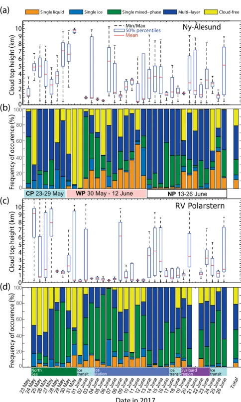
If the phase index is larger than 20, then the cloud is composed of ice particles, while a phase index less than 20 is an indication of a liquid water cloud. In the presented example, the phase index ranges mostly below 20 except where the cloud is optically thin, indicated by a low cloud reflectivity. The phase index map is in accordance with the lidar observations showing Fig. 7. Daily averaged time series of cloud type categorization resulting from

the Cloudnet algorithm for measurements taken at (a),(b) Ny-Ålesund and on (c),(d) R/V Polarstern, between 23 May and 26 Jun 2017. (a),(c) The statistics of the cloud-top-height distribution of all clouds shown in (b) and (d), respectively. Red horizontal bars, whisker boxes, and the dashed bars show the mean, 50% per- centile, and maximum/minimum of the observed cloud-top heights of each day.

2 Hawk is a proper name with no specific meaning.

854 | MAY 2019

(15)

a liquid cloud layer in lower altitudes. The upper ice cloud is optically thin and therefore not seen by the AISA Hawk spectrometer. It would be visible only if the lower liquid cloud layer were optically thin.

FOUR PIECES OF THE ARCTIC CLOUD PUZZLE. During ACLOUD/PASCAL numer- ous measurements have been collected to unravel some pieces of the Arctic cloud puzzle. First, results regarding four of these pieces are discussed below.

These “appetizers” comprise preliminary findings and highlight selected problems and open questions.

The in-depth analyses of the ACLOUD/PASCAL data will be continued.

Puzzle piece 1: Cloud properties. Clouds play a major role in Arctic amplification. Their macrophysical and microphysical properties determine whether they warm or cool the subcloud layer, and how strong these effects are. Local differences of cloud macrophysical properties, issues of ice formation in relatively warm clouds, and differences in ice occurrence in clouds over open ocean and sea ice are discussed in this subsection.

cloudMacrophysicalproperties—localdifferences. Figure 7 shows data derived from surface-based profile measurements with lidar, cloud radar, and a microwave radiometer. The measurements were collected at the AWIPEV site in Ny-Ålesund and at the R/V Polarstern. They were utilized for daily cloud classification with the Cloudnet categorization algorithm (Illingworth et al. 2007) for the period of the ACLOUD and PASCAL campaigns (23 May–26 June 2017). Each observed profile was checked for cloud phase between cloud bottom and cloud top. When only liquid water was detected within a single cloud layer, it was considered a single-layer liquid water cloud (single liquid). The same procedure was applied to single-layer ice clouds (single ice). If both cloud liquid water and ice phases were detected in one layer, then the cloud was counted as a single-layer mixed-phase cloud (single mixed phase). Samples with more than one detected layer separated by more than two 30-m-high bins correspond to multilayer clouds (multilayer). Additionally, “cloud free” events were classified.

Figures 7a and 7b illustrate the temporal evolution of cloud-top height and type statistics as observed at Ny-Ålesund. At the end of May (during the CP), the near-surface air temperature was much lower than later during the campaigns; therefore, the single ice and single mixed-phase clouds were more frequent

than in the first half of June (during the WP). During this WP the clouds occurred predominantly in the lower and midtroposphere, even though the spread of the cloud-top-height distribution was rather large. In the second half of June (during the NP), an increas- ing amount of single liquid clouds were observed as a result of warmer synoptic conditions. Either single mixed-phase or multilayer clouds were present throughout most of the time. These clouds were mostly formed in the lower troposphere and were likely caused by the presence of a strong temperature inversion, which is expected under high pressure conditions (Knudsen et al. 2018).

Figures 7c and 7d present corresponding results derived from measurements on the R/V Polarstern.

The most striking feature from the comparison of the R/V Polarstern and the Ny-Ålesund data is that single liquid clouds were observed less frequently above the R/V Polarstern. In turn, more mixed-phase clouds were detected over the research vessel. This can be attributed to the location of the R/V Polarstern, which was 400 km north of Svalbard, where temperatures were on average lower, favoring ice formation. The R/V Polarstern observations were made in closed sea ice, while Ny-Ålesund had open ocean west of the coast. When the R/V Polarstern passed Svalbard on 31 May 2017 (120 km west of Ny-Ålesund), cloud conditions at both measurement sites were rather similar. However, in contrast to Svalbard, low and partly mixed-phase fog was present over the R/V Polarstern for a couple of hours. Also, it can be seen in the R/V Polarstern observations that fewer cloud-free periods were sampled, which can be attributed to the higher frequency of occurrence of low-level fog over the edge of the sea ice, which is also indicated by the higher frequency of occurrence of low-level clouds shown in Fig. 7c.

These data show important local differences in cloud macrophysical properties, which need to be considered in the evaluation of cloud effects on their radiative energy budget and, thus, on Arctic amplification.

Microphysical cloud properties and in-cloud teMperatures—issues of iceforMation. To quantify the ranges of liquid/ice water contents and in-cloud temperatures encountered during the combined ACLOUD/PASCAL campaigns, Fig. 8 depicts prob- ability density functions (PDFs) for liquid water content (LWC; Fig. 8a), obtained from measurements of the Nevzorov probe and a combination of the cloud droplet probe (CDP) and cloud imaging probe (CIP), as well as ice water content (IWC; Fig. 8b) and