S F B
XXX
E C O N O M I C
R I S K
B E R L I N
SFB 649 Discussion Paper 2014-057
A Tale of Two Tails:
Preferences of neutral third-parties in
three-player ultimatum games
Ciril Bosch-Rosa*
*Technische Universität Berlin, Germany
This research was supported by the Deutsche
Forschungsgemeinschaft through the SFB 649 "Economic Risk".
http://sfb649.wiwi.hu-berlin.de ISSN 1860-5664
SFB 649, Humboldt-Universität zu Berlin
SFB
6 4 9
E C O N O M I C
R I S K
B E R L I N
A Tale of Two Tails: Preferences of neutral third-parties in three-player ultimatum games
Ciril Bosch-Rosa
∗First version: 13/2/2011 This Version: 31/10/2013
Abstract
We present a three-player game in which a proposer makes a suggestion on how to split $10 with a passive responder. The oer is accepted or rejected depending on the strategy prole of a neutral third-party whose payos are independent from his decisions. If the oer is accepted the split takes place as suggested, if rejected, then both proposer and receiver get $0. Our results show a decision-maker whose main concern is to reduce the inequality between proposer and responder and who, in order to do so, is willing to reject both selsh and generous oers.This pattern of rejections is robust through a series of treatments which include changing the at-fee payo of the decision-maker, introducing a monetary cost for the decision-maker in case the oer ends up in a rejection, or letting a computer replace the proposer to randomly make the splitting suggestion between proposer and responder. Further, through these dierent treatments we are able to show that decision- makers ignore the intentions behind the proposers suggestions, as well as ignoring their own relative payos, two surprising results given the existing literature.
JEL: C92, D71, D63, D31
Keywords: Ultimatum game, experiment, fairness, third party
∗Department of Economics, Technische Universität Berlin. Email: cirilbosch@gmail.com. I am greatly indebted to Johannes Müller- Trede for running some of the Barcelona experiments and for endless discussion over Skype. I would like to thank Robin Hogarth and Eldar Shar for guidance in the initial stage of this research, and Daniel Friedman, Nagore Iriberri, Rosemarie Nagel and Ryan Oprea for guidance at dierent stages. I would also like to thank Pablo Brañas and Teresa Garcia for their invaluable comments and help.
Thank you also to Gabriela Rubio for all the help and support. I am also grateful to Circe Bosch for help in making this a readable manuscript. Finally I'd like to acknowledge that discussants at ESA meetings in Copenhagen and Tucson as well as at Universidad de Granada's seminar were of great help. This project was partially funded by the Deutsche Forschungsgemeinschaft (DFG) through the SFB 649 "Economic Risk"
1 Introduction
How selsh soever man may be supposed, there are evidently some principles in his nature, which interest him in the fortune of others, and render their happiness necessary to him, though he derives nothing from it except the pleasure of seeing it. The Theory of Moral Sentiments, Adam Smith (1759)
Decisions made by uninvolved third-parties are not only an essential part of our judicial system, but are also central in many other more mundane activities. From a Supreme Court justice deciding over the Bush vs. Gore 2000 election results, to a building superintendent determining what neighbor is right in a noise complaint, neutral third parties impact our daily lives at many dierent levels. In fact, some studies claim that neutral third-parties should be ever more present in school conicts as it promotes social cohesion and reduces bullying (Cremin(2007);
Turnuklu et al. (2009)). Yet, very little work has been done on how the preferences of neutral third-parties look like.
In an eort to help shine some light on this topic we introduce a new three-player ultimatum game. In it a proposer makes an oer on how to split $10 with a responder who plays no role in the game. Meanwhile, and without knowing the suggestion made by the proposer, a neutral decision-maker lls in a strategy prole accepting or rejecting all the potential oers the proposer can make. If the oer is accepted, then the split takes place as suggested; if rejected, then both proposer and responder get $0. The decision-maker is paid a at fee independent of his choices.
We use an ultimatum game setup to study this topic because a bargaining game is a simple way of modeling a neutral third-party intervention, and because we can use previous references as benchmark. In addition, in our ultimatum setup a rejection by the decision-maker leaves both proposer and responder with a $0 payo, which constitutes a strong disagreement signal on behalf of the neutral third-party.
The rst result of our experiment shows that neutral decision-makers not only reject selsh oers, but they also refuse a substantial number of generous ones1. This appears to contradict previous results on three player games (Fehr and Fischbacher (2004) or Falk et al. (2008)) where neutral decision-makers rewarded generous oers and only punished selsh ones. To further look into it we introduce a series of robustness tests which include imposing a cost on the decision-maker if the game ends in a rejection, or having a computer replace the proposer, so that the splitting proposal (between proposer and responder) becomes random. These additional tests help us conrm our initial nding, and, most importantly, they show that proposers ignore the intentions behind a proposal, be them
1From now on we will consider any oer of more than$5to be generous.
generous or selsh. It seems thus that decision-makers seem to care only for equality, making our results even more at odds withFehr and Fischbacher(2004) orFalk et al. (2008).
If neutral decision-makers do ignore intentions as in our experiment, this should be of some concern for insti- tutions that rely on neutral referees, as intentions of defendants play an important role in most legal systems (e.g.
mens rea in criminal law,Martin(2003)). For instance, intentions are crucial in distinguishing between murder and manslaughter2, and in most universities not only is cheating a violation of the honor code, but so is attempting to cheat. Whenever neutral decision-makers do not care about intentions and are only concerned about the nal result of the game3 it may be necessary to introduce some mechanism in our institutions to help correct the indierence towards the intentions of other players.
The paper is organized in the following way. In section 2 we cover the existing literature on the subject. Section 3 describes both the baseline game and the dierent treatments. Sections 4 describes our results. Section 5 discusses some methodological points of the experiment, and nally we conclude in section 6.
2 Literature Review
Three-player games are an essential part of the ultimatum game literature, and have been responsible for some key insights in the topic. In Knez and Camerer(1995), a proposer makes a simultaneous oer to two independent responders who can accept or reject proposals conditional on the oer made to the other receiver. The results show that responders are not willing to get oered less than their counterpart. InGüth and van Damme(1998), a proposer splits the pie with a decision-maker and a passive dummy player who plays no role in the game; if the oer is accepted, then the split goes as suggested, if rejected, then everyone receives zero. The result is that both proposer and responder end up ignoring the presence of the dummy player and split the pie between themselves.
Finally,Kagel and Wolfe(2001) present us with a setup identical toGüth and van Damme(1998) except that now, if the oer is rejected, the dummy player gets a consolation prize. As inGüth and van Damme(1998), the dummy seems to play no role in the decision-makers mind, even when he gets a high consolation prize.
Many papers deal with the reasons behind the rejections of oers in two-player (and sometime three-player) bargaining games; from inequality aversion (Ockenfels and Bolton(2000) orFehr and Schmidt (1999)), to punish- ment of selsh intentions (Blount (1995);Falk et al.(2005)), or Rawlsian preferences (Charness and Rabin(2002);
Engelmann and Strobel(2004))4, and even to the need for signaling discomformity (Xiao and Houser(2005)). But
2A distinction as old as 624 BCE when Draco drafted the rst Athenian constitution and for the rst time distinguished between these two termsEhrenberg(1973)
3In our previous examples, whether or not someone is dead, or if the student actually copied or not.
4Which cannot really explain rejections in ultimatum games.
the literature grows silent when we look at the preferences of neutral third parties. Fehr and Fischbacher (2004) design a variation of the dictator game where a proposer oers an amount to a receiver, while a neutral third party can impose a (costly) punishment on the dictator. The results show that third party punishment is aimed to punish norm violators (i.e. selsh dictators) and not necessarily based on payo dierences among players.
On the other handLeibbrandt and Lopez-Perez(2008) use a within-subject analysis which shows that second and third party punishment are driven by payo dierences rather than the intentions of the proposer. Interestingly, and againstFehr and Fischbacher(2004), they also nd that second and third-party punishments are not signicantly dierent in intensity5. More recently, Falk et al.(2008) have revisited the subject suggesting that while inequality has some eect on punishment, intentions of the proposer are the main reason behind most punitive actions. Our conclusions are in stark contrast with these latter results as we nd that not only a signicant number of generous oers are rejected by third parties, but that (againstBlount(1995)) there are no statistical dierences between the rejections to oers made by another subject, and those made randomly by a computer.
And, while we are not the rst to report rejections of generous oers, we are the rst to do so in a lab experiment.
All previous reports of it were eld experiments with subjects either from rural old Soviet Union regions (Bahry and Wilson (2006)) or small-scale societies in New Guinea (Henrich et al. (2001)). Furthermore, these previous results had always been 2 player games, and considered an anomalies. For example, Bahry and Wilson (2006) dismiss rejections of generous oers as a result of Soviet education, while Henrich et al. (2001) hypothesize that these rejections could be the result of a gift-giving culture, in which accepting large gifts establishes the receiver as a subordinate. Güth et al.(2007) also mention an inverted-U in ultimatum game data gathered through newspaper publications. Yet, they only informally mentioned it because of the small number of observations following this pattern.
Finally, there has been some controversy about the validity of the strategy method, a technique which we use in our experiment. Brandts and Charness(2011) is a good survey on the subject and supports the use of the strategy method. In fact, if we had used a direct method instead of the strategy method, the inverted-U results might have been even more prominent asBrandts and Charness(2011) report that punishment rates are lower if the strategy method is used. Further, Brandts and Charness (2011) claim that in no case do we nd that a treatment eect found with the strategy method is not observed in the direct-response method. See also Brandts and Charness (2000) for more information on the matter.
5Fehr and Fischbacher(2004) show that second-parties spend much more of their income to punish unfair dictators
3 Experimental Design
The experiment was run with a total of 282 undergraduates from both the Universitat Pompeu Fabra (UPF) in Barcelona, and the University of California Santa Cruz (UCSC) in Santa Cruz. Each session had 3 rounds and lasted on average 30 minutes. The mean earnings at UCSC were of$4.5 and at UPF of ¿4.35plus a show-up fee ($5and ¿36) that was announced only at the end of the experiment7. Subjects were recruited through the ORSEE systems of each university (Greiner (2004)), and were required not to have any previous experience in bargaining games. In total 17 sessions were run, UCSC sessions had 12 subjects8 and UPF sessions 18 subjects9.
As subjects arrived to the lab, they were seated randomly in front of a terminal and the initial instructions were read aloud. In these instructions we announced that:
1. The experiment had three rounds and instructions for each round would be read immediately before each round started10.
2. Each subject would be assigned a player type (A, B or C) which they would keep through the experiment.
3. Each round, subjects would be randomly assigned to a dierent group of three players (one of each type).
4. Only one of the rounds, randomly chosen by the computer, would be chosen for the nal payos.
5. No feedback would be given until the end of the session11, when they would be informed of the actions of subjects in their group for each round, as well as the round selected for the nal payos.
Our experiment has a baseline treatment, and then 2 dierent robustness tests whose aim is to see how far we can push the results of the original treatment. Details on ordering and number of observations for each session can be found in Appendix A. A time line of the experiment is shown in Table 1.
6From now on, we will use the dollar sign to include both euros and dollars.
7While most subjects are aware of the rule of a show-up fee not announcing it until the end of the experiment adds pressure to the decision-makers would their decisions result in a rejection.
8Except 3 sessions that had 9 subjects.
9Except 2 sessions that had 12 subjects
10From experience, we prefer to read several times small amount of instructions rather than going over all instructions at the beginning of the session since subjects then get distracted. By breaking instructions into small concise parts we increase the likelihood that subjects are paying attention and, consequently, that they know what is expected of them in each round.
11This was done to minimize learning eects and have results of a one-shot game in each round.
Table 1: Steps of the experiment.
Step 1 Step 2 Step 3 Step 4
Read general instructions Read instructions for Round 1 Round 1 Read instructions for Round 2 Assign player type Assign players to group No feedback Assign players to new group
Step 5 Step 6 Step 7 Step 8
Round 2 Read instructions for Round 3 Round 3 Info on results for all games
No feedback Assign players to group No feedback Final payo info
3.1 Baseline
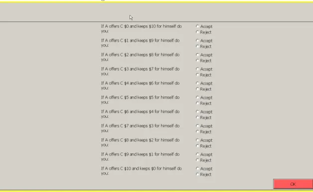
In the baseline design A players are assigned the role of proposer and have to make an oer on how to split $10 with a C player who is a bystanders and plays no active role in the game. In the meantime (and without knowing the proposal made by A) B players are assigned the role of decision-makers and have to ll in a strategy prole accepting or rejecting all potential oers from A to C (screen-shot in Figure 1). If the oer is accepted, the split goes as suggested by A; if rejected, then both A and C get $0 for the round. B player payos will be the treatment variable and these are:
Low (L): B gets paid $3 for his decisions, whatever the outcome of the game
Normal (N): B gets paid $5 for his decisions, whatever the outcome of the game.
High (H): B gets paid $12 for his decisions, whatever the outcome of the game.
Figure 1: Decision-Maker Screen-shot
Treatments L, H, and N allow us to test whether or not decision-makers take into account their relative payo when making the accept/reject decision. If no dierences can be observed across treatments, then it will mean that we are observing the revealed preferences of a subject who has truly no strategic or monetary concerns in the game;
what Fehr and Fischbacher(2004) call truly normative standards of behavior. Figure 2 graphically lays out the general structure of the baseline game.
Figure 2: General Structure of the Baseline Game
3.2 Robustness tests
Our robustness tests are variations of the baseline and were introduced to put to a test the unexpected results of our original treatments. In order to do this, we will use the H and L treatments of the baseline and adapt them to our new games, while using N will be used as the measure to which we will compare all the dierent treatments in the experiment.
3.2.1 Costly rejection
In this robustness test we have the exact same setup as the baseline, except that now if the game ends in a rejection, then the decision-maker is penalized by a subtraction of $1 from his payo for this round. So the treatments in the costly costly rejection sessions are:
Low (L-1) : B gets paid $3 if A's oer is accepted and $2 if rejected.
High (H-1) : B gets paid $12 if A's oer is accepted and $11 if rejected.
3.2.2 Computer
In the computer robustness test we have the same setup as in the baseline treatment, but this time the suggestion on how to split the $10 is randomly12 made by the computer. This leaves both A and C as bystanders13, while B lls in his strategy prole as usual. If the oer is accepted, then the split takes place as suggested by the machine, if rejected, then both A and C get $0. B's payos are completely independent from his choices and are:
Low (Lm): B gets paid $3 for his decisions, whatever the outcome of the game.
High (Hm): B gets paid $12 for his decisions, whatever the outcome of the game.
3.3 2UG
Finally, in all sessions one of the rounds will be the 2UG game. This game is designed to be a regular ultimatum game but keeping the 3-player group structure, as now A makes two independent suggestions on how to split$10;
12Following a uniform distribution across the whole oer space.
13Note that A is still a (human) subject getting a payo that depends on the decisions made by B and the random split suggested by the computer.
one to B, the other to C. As in the baseline, we use the strategy method to elicit both B and C's preferences over the oers made to them. If B (C) rejects the oer that A made to him, then B (C) gets$0 for the round. If, instead B (C) accepts the oer, then the split goes as suggested by A. A's payo is randomly chosen from one of the two dierent outcomes; if the selected game turns out to be a rejection, then A gets$0for the round, if an acceptance, then A gets his part of the proposal. The purpose of randomizing A's payos is to prevent portfolio eects and to make payos fair across all subject types.
The 2UG game is introduced in our sessions for three reasons. The rst one is to create a break between our treatments of interest14and so be able to recreate a rst-shot scenario in the third round of the session. Secondly we use the 2UG as a control for our population sample, and to verify whether or not our subjects understand the strategy method interface. Finally, and very important for our results, the 2UG game shows that decision-makers take seriously the possibility of generous oers when lling out their strategy prole.
4 Results
The analysis of our data begins by looking at the baseline treatments in section 4.1, to then study the results of both robustness tests in section 4.2. Finally we discuss our general results and experimental design in section 5, and conclude in section 6. The 2UG outcomes can be found in Appendix B, where we show that our sample is not dierent from that of any other ultimatum-game experiment, and that subjects understand perfectly the instructions and interface.
4.1 Baseline
Figure 3 presents the percentage of acceptances for each potential oer. In the upper-left corner we see the treatment N and in a clockwise order the comparison between N and L, L and H, and nally between N and H in the lower-left quadrant. Two things stand out immediately from these graphs. First, in all treatments there is a signicant amount of rejections of both selsh and generous oers. In fact, if an oer is generous, the more generous it is, the less likely that it will be accepted15.
Second, whether we pay a at-fee of$3or$12, both treatments show a very similar pattern of rejections. In fact, the rates of acceptance for each oer are not statistically dierent (Results for a Two-sided Fisher test can be found in Appendix C), and subjects seem to be consistent in their choices across treatments. A Wilcoxon matched-pairs signed-rank test presents us with no statistical dierences when comparing the number of acceptances made by the same subject participating in an N or an L treatment (p-value = 0.375) nor among those taking part in N and H
14Some 2UG rounds are at the beginning of the session just to show that there are no ordering eects.
15Thus creating the inverted-U shape thatBahry and Wilson(2006) rst identied in their eld experiments.
Figure 3: Acceptance Rates for Baseline Treatments
(p-value = 0.161)16, showing that decision-makers have stable preferences across treatments.
To further analyze our results, we run a regression of total accepted oers (Total) on dummies for location (Where), order (First), and treatment (High and Low). The results are in Table 2, with the rst two columns comparing treatment H to N, and L to N respectively. In the third and fourth columns, H and L are compared together to the N treatment. The results show that payos and order of treatments have no eect on the number of accepted oers17, and neither does location (all of these results are later conrmed in Table 3).
Table 2: Regression of total accepted oers by subject and treatment.
(1) Total (2) Total (3) Total (4) Total
Low -1.093 -1.327 -0.330 0.165
(0.848) (0.817) (0.666) (0.796)
First 1.707∗ 1.008
(0.947) (0.717)
Where -0.101 -0.263
(1.281) (0.979)
High 0.763 1.399
(0.805) (0.978) cons 6.593∗∗∗ 6.318∗∗∗ 5.830∗∗∗ 5.114∗∗∗
(0.747) (0.637) (0.461) (0.816)
∗p <0.10,∗∗p <0.05,∗∗∗p <0.01
It is thus apparent that decision-makers do not take their own payo into account when making decisions, which
16On the other hand, the test becomes somewhat more signicant when comparing L and H (p = 0.0825), probably because the number of subjects participating in both H and L is extremely low (n = 4). See Appendix D for a lengthier discussion on this question.
17Column 2 shows some minimal order eects. We attribute these to the lack of rst round H treatment observations. See Appendix D.
means that with our game design we are able to study the preferences of a neutral third-party with no strategic or monetary concerns in the game.
Result 1: In the baseline game there is no statistical dierence in rejection patterns across the dierent treatments, indicating that decision-makers ignore their payos when making decisions.
To better understand the data we dene absolute inequality as the absolute value of the dierence between A and C's payo. Then we label all oers to the left of $5 (the selsh oers) as those in the Left-Hand-Tail (LHT), and all oers to the right of $5 (the generous oers) as those in the Right-Hand-Tail (RHT). A Spearman rank correlation test (Appendix E) shows a strong positive (and monotonic) relationship between the increase in absolute inequality and the rejection rate, which means that in both tails, the bigger the inequality in the split, the lower the chance of the oer being accepted.
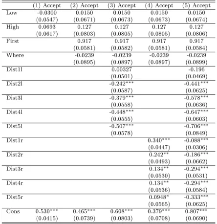
We also run a linear probability model18 (Table 3) where the binary accept/reject outcome is the dependent variable, and we have dummies for order (First), treatment (High, Low), location (Where), as well as dummies for distance. The coding for the distance dummies includes the distance to the even split and the tail they are in. So, for example, dist3l is the dummy for the $2 oer (which is 3 dollars to the left of $5) and dist2r is the dummy for an oer of $7(which is 2 dollars to the right of$5). Column 5 of Table 3 has the full specication of the regression, and as we can see that all dummies for distance are negative and highly signicant. Moreover, if we look at the coecients for the distance dummies, the further away an oer is from$5the lower the probability of being accepted. This relationship is monotonic in both tails19 ranging from an8%lower probability of acceptance for an oer of $6 (dist1r) to a 33.3%lower probability of acceptance for an oer of $10 (dist5r) when comparing them to the probability of acceptance of the even split$5.
As we can see, the decision-maker's preferences for equality are so strong that not only are they willing to leave the proposer and responder with a $0 payo when the oer is selsh, but they are also willing to leave them with
$0 if the oer is too generous.
Result 2: The greater the absolute inequality the lower the probability of the proposal being accepted.
However, in Figure 3 we see that the inverted-U is not perfectly symmetric around the fair split, as there is a higher number of acceptances in the RHT (generous oers) than in the LHT (selsh oers). This might mean
18With clustered errors at the individual level.
19Strictly monotonic in the LHT and weakly in the RHT, conrming the Spearman rank correlation results.
Table 3: Linear Probability model of Accepted Oers.
(1) Accept (2) Accept (3) Accept (4) Accept (5) Accept
Low -0.0300 0.0150 0.0150 0.0150 0.0150
(0.0547) (0.0671) (0.0673) (0.0673) (0.0674)
High 0.0693 0.127 0.127 0.127 0.127
(0.0617) (0.0803) (0.0805) (0.0805) (0.0806)
First 0.917 0.917 0.917 0.917
(0.0581) (0.0582) (0.0581) (0.0584)
Where -0.0239 -0.0239 -0.0239 -0.0239
(0.0895) (0.0897) (0.0897) (0.0899)
Dist1l 0.00327 -0.196
(0.0501) (0.0469)
Dist2l -0.242∗∗∗ -0.441∗∗∗
(0.0587) (0.0625)
Dist3l -0.379∗∗∗ -0.578∗∗∗
(0.0558) (0.0636)
Dist4l -0.448∗∗∗ -0.647∗∗∗
(0.0555) (0.0603)
Dist5l -0.507∗∗∗ -0.706∗∗∗
(0.0578) (0.0849)
Dist1r 0.340∗∗∗ -0.088∗∗∗
(0.0447) (0.0306)
Dist2r 0.242∗∗ -0.186∗∗∗
(0.0493) (0.0662)
Dist3r 0.134∗∗ -0.294∗∗∗
(0.0530) (0.0531)
Dist4r 0.134∗∗ -0.294∗∗∗
(0.0536) (0.0584)
Dist5r 0.0948∗ -0.333∗∗∗
(0.0565) (0.0625) Cons 0.530∗∗∗ 0.465∗∗∗ 0.608∗∗∗ 0.379∗∗∗ 0.807∗∗∗
(0.0415) (0.0739) (0.0803) (0.0708) (0.0690)
∗p <0.10,∗∗p <0.05,∗∗∗p <0.01
that decision-makers care about the intentions of proposers. To check the extent of this asymmetry, we run a linear probability model for each treatment (H, N, L), and compare the coecients of the oers with same absolute inequality through a Wald Test (Table 4). The results show that in all the treatments the tails are asymmetric, with a higher degree or rejections on the selsh side (LHT). A Two-sided Fisher test comparing the number of accepted oers for same absolute inequality proposals conrms this result (Appendix F).
Table 4: P-values of Wald test for equality in within treatment regression coecients.
Treatment dist1l=dist1r dist2l=dist2r dist3l=dist3r dist4l=dist4r dist5l=dist5r
L 0.3357 0.0187∗∗∗ 0.0052∗∗∗ 0.0026∗∗∗ 0.0013∗∗∗
H 0.5813 0.0066∗∗∗ 0.0186∗∗∗ 0.0016∗∗∗ 0.0016∗∗∗
N 0.0107∗∗ 0.0021∗∗∗ 0.0022∗∗∗* 0.000∗∗∗ 0.000∗∗∗
∗p <0.10,∗∗ p <0.05,∗∗∗p <0.01
Result 3: In the baseline treatments, decision-makers are less willing to tolerate inequality when it is the result of a selsh oer.
The three results presented above oer a picture of a decision-maker who does not seem to care about his relative payo, but who is extremely concerned with the inequality between proposer and responder, as well as showing some dislike for selsh oers.
4.2 Robustness Tests
In this sections we analyze both robustness tests. The rst one is the costly-rejection game. The design is identical to the baseline, except that now the decision-maker has to pay a$1penalty if the game ends in a rejection20. This test was introduced to put downward pressure on the number rejections that B players make. If we still observe rejections of both selsh and generous oers in spite of the penalty, then this may be taken as a strong indication of the commitment of decision-makers towards equality. Also, the introduction of this penalty allows us to get a sense of what type of concerns, whether intentions of the proposer or absolute inequality, are more fragile in the decision-maker's preference set. If it happens that intentions play a stronger role than absolute inequality aversion, then we should observe acceptance in the RHT go up relative to those in the LHT. On the other hand, if inequality aversion is more important than intentions, then the result of introducing a penalty should be a much more symmetric pattern of rejections in this treatment than in the baseline game.
The second robustness check is the computer game. Again, we maintain the baseline design, but now the oer from A to C will be randomly chosen by a computer21. Because there are no intentions ingrained in the oers, but there still might be inequality, we expect to nd a symmetric distribution of acceptances around the even split. Yet, what will be important in this game is the statistical comparison between the baseline and the computer treatment; if there is no statistical dierence between them, then it will mean that intentions have very little weight in the decision-maker's preferences. If there is, then it will mean that intentions are (signicantly) important for decision-makers.
4.2.1 Costly-Rejection
In Figure 4 we present the results of the costly-rejection treatments and compare them to their baseline counterparts and with the N treatment. The rst thing that catches our attention is that, even when rejections are costly to decision-makers, we still observe them in both tails, following the same negative monotonic pattern that we already saw in the baseline treatment22.
20Details can be found in section 3.2.1.
21Details can be found in section 3.2.2.
22See Appendix G for Spearman Correlation results
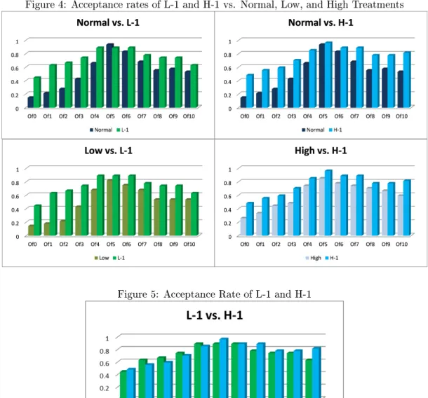
Figure 4: Acceptance rates of L-1 and H-1 vs. Normal, Low, and High Treatments
Figure 5: Acceptance Rate of L-1 and H-1
Furthermore, the similarity between H-1 and L-1 is striking (detail in Figure 5). Running a Wilcoxon matched- pairs sign-rank test comparing the number of accepted oers in each treatment, we nd that the decision-maker's behavior is not statistically dierent across treatments (p-value = 0.6172). Additionally, both the linear probability model of Table 5 and a Two-sided Fisher test (Appendix H), conrm that there exists no signicant dierence between treatments. So, even when the relative costs of rejecting oers are wide apart, decision-makers behave in a similar manner under both costly treatments.
Result 4: Even with widely dierent relative rejection costs, there is no signicant dierence across treatments in the Costly-Rejection game.
Table 5: Linear Probability model of Accepted Oers.
(1) Accept (2) Accept (3) Accept (4) Accept (5) Accept
High1 0.0236 0.0289 0.0289 0.0289 0.02889
(0.0615) (0.0671) (0.0674) (0.0674) (0.0677)
First 0.0236 0.0289 0.0289 0.0289 0.02889
(0.0615) (0.0671) (0.0674) (0.0674) (0.0677)
Dist1l 0.0556 -0.0556
(0.0417) (0.0412)
Dist2l -0.0926∗∗∗ -0.204∗∗∗
(0.0391) (0.0675)
Dist3l -0.185∗∗∗ -0.296∗∗∗
(0.643) (0.0820)
Dist4l -0.222∗∗∗ -0.333∗∗∗
(0.0595) (0.0809)
Dist5l -0.352∗∗∗ -0.463∗∗∗
(0.0697) (0.0849)
Dist1r 0.188∗∗∗ -0.0370
(0.0574) (0.0461)
Dist2r 0.133∗∗ -0.0926
(0.0493) (0.0662)
Dist3r 0.0585 -0.167∗∗
(0.0500) (0.0763)
Dist4r 0.0585 -0.167∗∗
(0.0462) (0.0660)
Dist5r 0.0216 -0.204∗∗∗
(0.0487) (0.0675) Cons 0.731∗∗∗ 0.713∗∗∗ 0.786∗∗∗ 0.672∗∗∗ 0.897∗∗∗
(0.0608) (0.0840) (0.0809) (0.0893) (0.0860)
∗p <0.10,∗∗p <0.05,∗∗∗p <0.01
On the other hand, we do see some dierences when comparing the costly rejections treatments and their baseline counterparts. Running a regression on total accepted oers comparing H to H-1 and L to L-1 we see signicant dierences (p= 0.002 and p = 0.000 respectively) for their treatment dummies.
From Figure 4 it seems that most dierences across baseline and robustness treatments stem from an increase of acceptances in the LHT. Apparently, when a cost is introduced, decision-makers accept relatively more selsh oers, while keeping a similar rate of rejections for the generous ones. To test this interpretation, we run a one-sided Fisher test comparing the number of accepted oers for each potential splitting suggestion, and conrm that the dierences are mostly in the LHT (Table 6). Therefore we conclude that decision-makers have only some weak concern for the intentions of the proposer, while their absolute inequality aversion seems pretty robust, as the introduction of a cost has almost no eect on the latter but it increases signicantly acceptance rates in the former.
This conclusion is supported by a Wald test comparing the coecients of the oers that have the same level of absolute inequality (Table 7). The results show a symmetric L-1, but a slightly unbalanced H-1. A Two-sided Fisher (Table 8), shows symmetry under both treatments.
Table 6: One-sided Fisher P-values comparing total acceptances per treatment.
$0 $1 $2 $3 $4 $5 $6 $7 $8 $9 $10
L vs. L-1 0.01∗∗ 0.01∗∗ 0.01∗∗ 0.01∗∗ 0.05∗ 0.37 0.16 0.30 0.09∗ 0.09∗ 0.33 H vs. H-1 0.07∗ 0.08∗ 0.20 0.08∗ 0.25 0.17 0.23 0.14 0.37 0.27 0.06∗
∗p <0.10,∗∗p <0.05,∗∗∗p <0.01
Table 7: P-values of Wald test
Treatment dist1l=dist1r dist2l=dist2r dist3l=dist3r dist4l=dist4r dist5l=dist5r
L-1 1.00 0.7536 0.5302 0.3466 0.1175
H-1 0.7410 0.0991∗ 0.0991∗ 0.0481∗∗ 0.0032∗∗∗
∗p <0.10,∗∗ p <0.05,∗∗∗p <0.01
Result 6: Under Costly-Rejection treatments, the intentions of the proposer play a minor role in the accep- tance pattern of decision-makers, its impact disappearing completely in the costlier case (L-1).
4.2.2 Computer Treatment
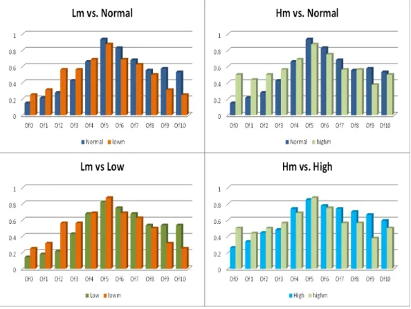
Figure 6 presents the results of this game and compares Hm to N and H in the right column, and Lm to N and L in the left column. It is apparent that all computer treatments are symmetric around the fair split ( a two-sided Fisher test comparing equal absolute inequality oers shows a p-value=1.000 for all cases in both treatments), so decision-makers do not dierentiate between the RHT and the LHT in this game.
Table 8: Two-Sided Fisher P-values.
Treatment $4=$6 $3=$7 $2=$8 $1=$9 $0=$10
L-1 1.000 1.000 0.766 0.559 0.275
H-1 1.000 0.175 0.241 0.148 0.021∗∗
∗p <0.10,∗∗ p <0.05,∗∗∗p <0.01
Figure 6: Acceptance rates of Lm and Hm vs. Normal, Low, and High Treatments
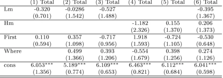
To compare the machine and baseline treatments we run a regression of total number of accepted oers on a dummy for treatment, location, and ordering in Table 9. The rst three columns compare the data of Lm to Hm, then to L, and nally to N. The fourth and fth column compare Hm rst to H and then to N, and the last column compares Hm and Lm together to the N treatment results. There appears to be no signicant dierences across treatment dummies, so independent of whether the oer was made by a human or a computer, the number of accepted oers are the same. A two-sided Fisher test in Appendix I conrms this result, as does column 3 of Table 9, where we run a linear probability model comparing the data of both Lm and Hm to N.
Result 7: Rejection patterns of oers made (randomly) by a computer are not statistically dierent from rejection patterns of oers made by a human being.
Table 9: Regression of total accepted oers by subject and treatment.
(1) Total (2) Total (3) Total (4) Total (5) Total (6) Total
Lm -0.320 -0.0286 -0.527 -0.395
(0.701) (1.542) (1.488) (1.367)
Hm -1.182 0.155 0.206
(2.326) (1.370) (1.373)
First 0.110 0.357 -0.717 1.918 -0.724 -0.530
(0.594) (1.098) (0.956) (1.593) (1.105) (0.648)
Where 0.499 0.393 -0.554 0.398 0.274
(1.366) (1.206) (1.679) (1.256) (1.126) cons 6.053∗∗∗ 5.189∗∗∗ 6.109∗∗∗ 6.463∗∗∗ 6.112∗∗∗ 6.041∗∗∗
(1.356) (0.774) (0.653) (0.821) (0.684) (0.598)
∗p <0.10,∗∗ p <0.05,∗∗∗p <0.01
So, while Result 3 found that intentions are somewhat important to decision-makers, Result 6 and Result 7 show that the weight that these have on acceptance rates is really small, especially when compared to how important absolute inequality appears to be.
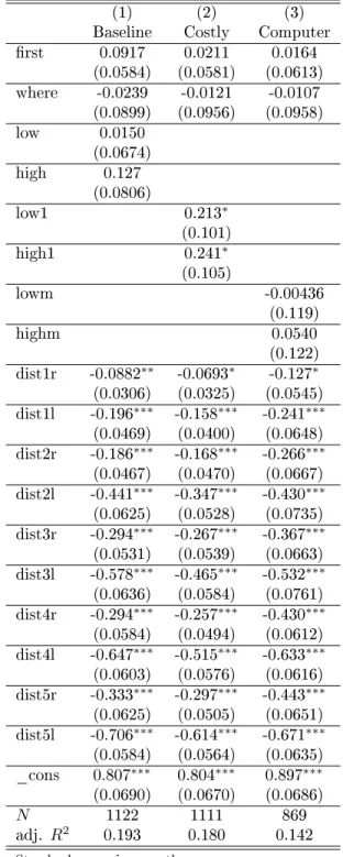
To oer an overall picture of this experiment, Table 10 presents a linear probability model comparing N to the high and low payo treatments of each game.23 The results show a signicant dierence of the costly rejection treatments when compared to the N baseline (both Low1 and High1 are signicantly dierent at the 5% in column 2), while neither the computer treatment nor the baseline treatments H and L are dierent from N. In all cases, again, distance from the fair split is highly signicant and the probability of acceptance decreases monotonically as oers get away from the fair split in either direction.
In summary, after testing the preferences of decision-makers across three dierent games, it is pretty cleat that the main motivation for rejecting an oer is to reduce the payo inequalities between players A and C. Intentions of the proposer, on the other hand, have only a minor eect in the baseline treatments where acceptance distributions are not perfectly symmetric around the $5 even split. Finally, when a cost for rejecting a proposal is introduced, rejection patterns dier from the pattern baseline treatment N, yet we do not observe signicant dierences between treatments H-1 and L-1.
23Please note that the p-value notation is changed in this table with respect to all other tables in the paper.
Table 10: Linear probability model comparing each treatment to baseline N treatment
(1) (2) (3)
Baseline Costly Computer
rst 0.0917 0.0211 0.0164
(0.0584) (0.0581) (0.0613) where -0.0239 -0.0121 -0.0107
(0.0899) (0.0956) (0.0958)
low 0.0150
(0.0674)
high 0.127
(0.0806)
low1 0.213∗
(0.101)
high1 0.241∗
(0.105)
lowm -0.00436
(0.119)
highm 0.0540
(0.122) dist1r -0.0882∗∗ -0.0693∗ -0.127∗ (0.0306) (0.0325) (0.0545) dist1l -0.196∗∗∗ -0.158∗∗∗ -0.241∗∗∗
(0.0469) (0.0400) (0.0648) dist2r -0.186∗∗∗ -0.168∗∗∗ -0.266∗∗∗
(0.0467) (0.0470) (0.0667) dist2l -0.441∗∗∗ -0.347∗∗∗ -0.430∗∗∗
(0.0625) (0.0528) (0.0735) dist3r -0.294∗∗∗ -0.267∗∗∗ -0.367∗∗∗
(0.0531) (0.0539) (0.0663) dist3l -0.578∗∗∗ -0.465∗∗∗ -0.532∗∗∗
(0.0636) (0.0584) (0.0761) dist4r -0.294∗∗∗ -0.257∗∗∗ -0.430∗∗∗
(0.0584) (0.0494) (0.0612) dist4l -0.647∗∗∗ -0.515∗∗∗ -0.633∗∗∗
(0.0603) (0.0576) (0.0616) dist5r -0.333∗∗∗ -0.297∗∗∗ -0.443∗∗∗
(0.0625) (0.0505) (0.0651) dist5l -0.706∗∗∗ -0.614∗∗∗ -0.671∗∗∗
(0.0584) (0.0564) (0.0635) _cons 0.807∗∗∗ 0.804∗∗∗ 0.897∗∗∗
(0.0690) (0.0670) (0.0686)
N 1122 1111 869
adj. R2 0.193 0.180 0.142
Standard errors in parentheses
∗p <0.05,∗∗ p <0.01,∗∗∗ p <0.001
5 Discussion
Neutral referees make complex decisions based on a number of dierent factors. Fehr and Fischbacher (2004) and Falk et al.(2008) postulate that (selsh) intentions the punishment of proposers. InLeibbrandt and Lopez- Perez (2008), on the other hand, envy is identied as the main reason behind third-party punishment. In our experiment we nd that the main concern of neutral third-parties is avoiding absolute inequality between proposer and responder. In fact, we nd that this concern is so strong that decision-makers are willing to punish both proposer and responder with a $0 payo if the oer is too generous, to avoid too big of an inequality between them.
Much of our data analysis is aimed at showing that there is no learning and no ordering eects in our results.
This is necessary precaution because we collect the data following a within-subject design, yet we use them as if they came from a between-subject experiment. The reason is that in a between-subject design we would have collected only one observation for every three subjects invited into the lab, making the experiment expensive and time-consuming. Thankfully, having managed to show that there are no ordering or learning eects, we can use our data as if they all came from rst-shot interactions. We believe that not giving feedback until the end of the session, mixing groups between rounds, paying only one round, and having the 2UG break are all crucial tools to avoiding any learning in our subjects.
Finally, we would want to mention that even though the number of observations for the computer treatment is not large, the results appear to be robust when tested in dierent ways.
6 Conclusion
Neutral third parties are everywhere in our institutions: from the members of the European Commission24deciding how to allocate the farming subsidies, to the referees of the Super Bowl, to the TV show Judge Judy25. Yet, as important as neutral third-parties are, the literature studying their preferences is still slim.
In an eort to help shine some light on this topic, we run an experiment introducing a new version of the three- player ultimatum game. In it a proposer makes an oer on how to split $10 with a responder who plays no role in the game. Meanwhile, and without knowing the suggestion made by the proposer, a neutral decision-maker lls in a strategy prole accepting or rejecting all the potential oers from the proposer. If the actual oer is accepted, then the split goes as suggested; if rejected, then both proposer and receiver get a payo of $0. The payo of the neutral third-party is independent of his decisions.
24Note that even if there is one commissioner per member state, these are expected to represent the interests of the EU and not their respective countries.
25This is a program where a retired judge decides over small-claim disputes, and where both plainti and defendant have previously signed a contract agreeing to accept the resolution of the judge.
The results of the experiment show that neutral decision-makers are mostly concerned with reducing the payo dierences between proposer and responder, even if this means rejecting a generous oers and leaving both subjects with a $0 payo. Similar rejections pattern had been previously reported in the eld (Bahry and Wilson(2006) and Henrich et al.(2001)), but never in the lab or in a three-player setting. This result challenges some of the previous literature such asFehr and Fischbacher(2004) orFalk et al.(2008), where third-parties reward generous oers and punish selsh ones.
To test the robustness of our results we introduce a number of variations to our original game. In a rst variation we charge the decision-maker $1 if the game ends in a rejection; in a second one we substitute the proposer by a computer that randomly proposes a split of the $10. In both cases we continue to observe rejections of generous and selsh oers, and cannot nd any statistical dierences between the original treatment and the two variations.
We, therefore, conclude that reducing absolute inequality26 is the main concern of the decision-makers, while the intentions of the proposer play only a secondary role.
The above mentioned results could be worrisome for institutions relying on the decisions of neutral third- parties, since in our experiment not only do they make extremely inecient decisions, but they also seem to ignore the intentions behind proposals. This latter nding, if general, could become a problem in our legal system where intentions and premeditation carry so much weight. And while it is beyond the scope of this paper to suggest a mechanism to correct the observed bias for equality in neutral third-parties, we believe that running further experiments in collaboration with faculty at Law Schools, or using subject pools composed by professional arbitrageurs or judges should be a natural next step. If such experiments conrmed our observations, in addition to inviting the appropriate institutional reforms, they would also no doubt promote the experimental method as a useful tool to improve legal regulation and institutions.
26As dened in section 4.1.
Appendix:
Appendix A: Details on session structure
The treatment ordering for each session as well as the total number of subjects per session in Table A.1 Treatment Order/Town Barcelona Santa Cruz
N2H 18 21
N2L 18 21
(H-1)2(L-1) - 33
(L-1)2(H-1) - 48
L2H - 12
2NL 18 -
2NH 18 -
H2N 15 -
L2N 15 -
Lm2Hm 30 -
Hm2Lm 18 -
Table 11: Treatment ordering and number of B subject observations
In Table A.2 we present the total number of actual decision-maker observations for each treatment:
Barcelona Santa Cruz Total
N 33 14 47
H 17 11 28
L 17 11 28
H-1 - 27 27
L-1 - 27 27
Lm 33 - 16
Hm 33 - 16
Table 12: Total number of B subject observations per treatment
Appendix B: 2UG Results
We summarize all of B subject's observations in Figure 7. In it we present the percentage of decision-makers accepting each potential oer from A to C (e.g. almost 60% of B subjects accept a hypothetical oer of $3while only 30% accept one of 1). The acceptance results are slightly higher than those reported in the literature (see Camerer and Thaler(1995)), but still within the range of what would be expected. The average oer was of $3.59, which is also what would be expected in an experiment like this. These results validate both our subject pool and the software interface, but most importantly, they show that decision-makers act consistently27when deciding
27Three subjects that rejected oers of $8 or more yet accepted all smaller oers. We believe that these subjects misunderstood the interface and were trying to reject oers smaller than$2.
about hyper-generous oers (i.e., subjects do not randomize or experiment within this range of oers). We take this as an indication that decision-makers take seriously the possibility of a generous oer.
Figure 7: Acceptances of 2UG
Appendix C: Two-sided Fisher test for baseline treatments
$0 $1 $2 $3 $4 $5 $6 $7 $8 $9 $10
L=H 1.000 0.775 0.596 1.000 1.000 0.141 0.550 1.000 1.000 0.810 1.000 H=N 0.355 0.280 0.202 0.808 0.604 0.250 0.759 0.792 0.226 0.469 0.636 L=H 0.329 0.227 0.089* 0.789 0.768 1.000 1.000 0.768 0.269 0.412 0.787
Table 13: Two-Sided Fisher P-values
Appendix D: Ordering Eects
Due to a miscommunication between the Barcelona and Santa Cruz labs we have a very unbalanced amount of for rst round H treatment (5) compared with third round H treatment (22). This unfortunately pollutes the ordering eects for the H treatments as a 2 tailed Fisher Test comparing rst round treatments against other rounds in the experiment shows.
$0 $1 $2 $3 $4 $5 $6 $7 $8 $9 $10
N 0.752 0.890 0.344 0.671 0.174 1.000 0.767 0.492 0.357 0.923 0.628 H-1 0.704 1.000 1.000 0.090* 0.621 1.000 1.000 1.000 1.000 1.000 1.000 H 0.091* 0.030** 0.010** 0.165 0.238 1.000 1.000 1.000 1.000 0.136 0.060*
L 0.574 1.000 0.352 0.687 0.407 1.000 1.000 1.000 0.435 1.000 0.435 L-1 1.000 0.448 0.692 1.000 0.056* 0.549 0.549 1.000 0.662 0.662 0.448
∗p <0.10,∗∗ p <0.05,∗∗∗p <0.01
Table 14: Two-Sided Fisher P-values Comparing First Round Treatments to all Other Treatments
While most treatments have no ordering eects, the LHT of the H treatment seems to be signicantly aected by ordering. If we look at Graph A, we can see that while last round pattern of acceptances does look like those in the rest of treatments, rst round H acceptances looks pretty random. As mentioned, we believe that this is due to the low number of observations of H in the rst round, and that if we had more observations we would see no ordering eects.
Figure 8: Acceptance Rates for H for First (n=5) and Third (n=22) Round
Appendix E: Spearman Rank Correlation
In order to test for the correlation between distance and acceptance rates we rst run a Spearman Rank Correlation test (Table 15) where a result of 1 or -1 is a perfect monotonic correlation of coecients (in this case distance and acceptances). To run this test we divide our support into two separate tranches, the rst one will include all oers to the left of $5 (LHT), the second tranche will include all oers to the right of ve (RHT). As we can see, the RHT has a perfectly linear and highly signicant relation between distance to the even split and acceptance levels;
the closer to $5, the more acceptances we see. In the RHT the correlation is almost as perfect, in this case we see how as we get further away from $5 the levels of acceptance fall in a highly signicant quasi-linear way.
Table 15: Spearman Rank Correlation Results for LHT and RHT under L, N and H treatments.
LHT(L) LHT(N) LHT(H) RHT(L) RHT(N) RHT(H) Spearman Rho 1.000 1.000 1.000 -0.9411 -0.9429 -1.000 Prob > |t| 0.000 0.000 0.000 0.0051 0.0048 0.0000
Appendix F: Two-sided Fisher Test comparing same absolute inequality oers across all treatments in the baseline
Table 16: Two-sided Fisher Test.
Treatment $4=$6 $3=$7 $2=$8 $1=$9 $0=$10
L 0.768 0.106 0.026∗∗ 0.011∗∗ 0.004∗∗∗
H 1 0.093∗ 0.098∗ 0.029∗∗ 0.027∗∗
N 0.048∗∗ 0.011∗∗ 0.006∗∗∗ 0.001∗∗∗ 0.0000∗∗∗
∗p <0.10,∗∗p <0.05,∗∗∗p <0.01
Appendix G: Spearman Rank Correlation
Table 17: Spearman Rank Correlation Results for LHT and RHT under L, N and H treatments.
LHT(L-1) LHT(H-1) RHT(L-1) RHT(H-1)
Spearman Rho 0.9856 1.000 -0.9710 -0.7495
Prob > |t| 0.0003 0.0000 0.0012 0.0059
Appendix H: Two-sided Fisher
$0 $1 $2 $3 $4 $5 $6 $7 $8 $9 $10
L-1 vs. H-1 1.000 0.782 0.779 1.000 1.000 0.610 1.000 0.467 1.000 1.000 0.224 Table 18: Two-Sided Fisher P-values Comparing First Round Treatments to all Other Treatments
Appendix I: One-sided Fisher Test for Machine Treatment
Table 19: One-sided Fisher P-values comparing total acceptances per treatment.
$0 $1 $2 $3 $4 $5 $6 $7 $8 $9 $10
L vs. Lm 0.434 0.456 0.026∗∗ 0.533 1.00 1.00 0.732 0.751 1.00 0.213 0.113 H vs. Hm 0.185 0.530 0.761 0.755 0.737 1.00 1.00 0.316 0.509 0.111 0.752
∗p <0.10,∗∗ p <0.05,∗∗∗p <0.01
Appendix J: Instructions L2H
Welcome! This is an economics experiment. You will be a player in many periods of an interactive decision-making game. If you pay close attention to these instructions, you can earn a signicant sum of money. It will be paid to you in cash at the end of the last period. It is important that you remain silent and do not look at other people's work. If you have any questions, or need assistance of any kind, please raise your hand and we will come to you.
If you talk, laugh, exclaim out loud, etc., you will be asked to leave and you will not be paid. We expect and appreciate your cooperation today.
This experiment has three dierent rounds. Before each round the specic rules and how you will earn money will be explained to you. In each round there will always be three types of players: A, B and C. You will be assigned to a type in Round 1 and will remain this type across all three rounds. Only one of the three rounds will be used for the nal payos. This round is chosen randomly by the computer. The outcomes of each round are not made public until the end of the session (i.e. after round 3). Each round the groups are scrambled so you will never make oers or decide for the same player in two dierent rounds.
Round 1:
The rst thing that you will see on your screen is your player type.
You will then be assigned to a group consisting of three players: an A type, B type and C type.
Player A will be endowed with $10 which he will split with player C. In order to do so Player A will have to input the amount he is willing to oer Player C. Player A will only be able to make integer oers (full dollars), so A will not be able to break its oer into cents.
While player A is deciding how much to oer player C, player B will be lling out a binding strategy prole.
The strategy prole has an accept or reject button for each potential oer from A to C (from $0 to $10). Player B's binding decision to accept or reject A's oers to C will be done before he knows the actual oer made by A.
A's decision: How to split an endowment of $10 with Player C by making him an oer between $0 and $10. If the oer is of $X, A will be keeping for himself 10-X.
B's decision: Before knowing the oer from A to C, B will ll a binding strategy prole deciding whether he accepts or rejects every potential oer from A to C. This decision is made without knowing the oer from A to C.
Figure 9: Diagram 3UG
It is very important for A to realize that he is going to write the amount he wants to oer C and not how much he wants to keep.
Payo for Round 1:
If B accepts the oer from A to C, then they split the $10 as suggested by A.
If B rejects the oer from A to C, then both (A and C) get $0.
B will get paid $3 no matter what is the outcome.
Timing and Payos:
1. B lls a strategy prole with all potential oers from A to C.
2. A decides how much to oer C (say X)
Figure 10: Diagram of Payos
Round 2:
As mentioned at the beginning of the experiment you will keep your player type across the whole session. So A players are still A, B are B and C are C.
In this round type A players will be endowed with $20 and will have to make TWO oers:
1. How to split $10 with player B.
2. How to split $10 with player C.
As in Round 1 a binding strategy prole will be lled by B and C players before they know the oer made to them.
It is very important to notice that B and C players are making decisions concerning their own payos.
A's decision: How to split $10 with B and how to split $10 with A.
Each oer is independent. So the outcome of the oer to B has no eect on the outcome of the oer to C.
Payos for A will be as in Round 1 (if he oers X and the oer is accepted he gets $10-X, if the oer is rejected both him and the rejecting player get 0).
B and C players will get paid X or 0 depending if the accepted or rejected the oer made directly to them.
In order to make payos equitable for this round, A's payo for this round will be chosen at random between one of the two outcomes (oer to B and oer to C). B and C's decision: Before knowing the oer made to them by Player A, B and C will ll a binding strategy prole deciding if they accept or reject every potential oer made directly to them.
If the oer from A is accepted, then the split is done as proposed by A. If the oer is rejected both the receiver and A get $0 as the outcome for this round.
Figure 11: 2UG Diagram
Timing and Payo for Round 2:
1. Each receiver lls a strategy prole with all potential oers that A could make them.
2. A decides how much to oer C and B (say X)
3. Payos for B and C will be the outcome of their particular game with A.
4. To make outcomes equitable, the computer will choose randomly one of the two outcomes to be A's payo for the round.
For each oer made from A to the other members of his group:
Figure 12: 2UG Payos
Round 3:
As mentioned at the beginning of the experiment you will remain your player type across the whole session.
This round is very similar to round 1. You will now be re-scrambled into groups of three subjects (one A, one B and one C subject).
A will be endowed with $10 and must decide how to split them with C.
B's role is exactly the same as that in round 1: Before knowing the oer from A to C, B will ll a strategy prole deciding whether he accepts or rejects every potential oer from A to C.
If the oer from A to C is accepted by B, then the split is done as proposed by A. If B rejects the oer, then both A and C receive $0 for this round.
B's payo in this round is a at $12 fee, whatever his decision and outcome of the round. So, the only change between Round 1 and Round 3 is that player B, is getting paid a dierent amount.
Figure 13: 3UG (H) Diagram
Timing and Payos:
1. B lls a strategy prole with all potential oers from A to B.
2. A decides how much to oer C (say X)
Figure 14: Payment Diagram 3UG (H)