does not in fl uence the atmosphere

Extensive release of methane from Arctic seabed west of Svalbard during summer 2014

does not in fl uence the atmosphere

C. Lund Myhre¹, B. Ferré², S. M. Platt¹, A. Silyakova², O. Hermansen¹, G. Allen³, I. Pisso¹,

N. Schmidbauer¹, A. Stohl¹, J. Pitt³, P. Jansson², J. Greinert^2,4,5, C. Percival³, A. M. Fjaeraa¹, S. J. O’Shea³, M. Gallagher³, M. Le Breton³, K. N. Bower³, S. J. B. Bauguitte⁶, S. Dalsøren⁷, S. Vadakkepuliyambatta², R. E. Fisher⁸, E. G. Nisbet⁸, D. Lowry⁸, G. Myhre⁷, J. A. Pyle⁹, M. Cain⁹, and J. Mienert²

1NILU-Norwegian Institute for Air Research, Kjeller, Norway,²CAGE-Centre for Arctic Gas Hydrate, Environment and Climate, Department of Geology, UiT - Arctic University of Norway, Tromsø, Norway,³Centre for Atmospheric Science, School of Earth, Atmospheric and Environmental Science, University of Manchester, Manchester, UK,⁴GEOMAR, Helmholtz-Zentrum für Ozeanforschung, Kiel, Germany,⁵Christian-Albrechts-University Kiel, Institute of Geosciences, Kiel, Germany,⁶Facility for Airborne Atmospheric Measurments (FAAM), Natural Environment Research Council (NERC), Cranfield, UK,⁷Center for International Climate and Environmental Research-Oslo (CICERO), Oslo, Norway,⁸Department of Earth Sciences, Royal Holloway, University of London, Egham, UK,⁹National Centre for Atmospheric Science, Department of Chemistry, University of Cambridge, Cambridge, UK

Abstract

^Wefind that summer methane (CH₄) release from seabed sediments west of Svalbard substantially increases CH₄concentrations in the ocean but has limited influence on the atmospheric CH₄levels. Our conclusion stems from complementary measurements at the seafloor, in the ocean, and in the atmosphere from land-based, ship and aircraft platforms during a summer campaign in 2014. We detected high concentrations of dissolved CH₄in the ocean above the seafloor with a sharp decrease above the pycnocline. Model approaches taking potential CH₄emissions from both dissolved and bubble-released CH₄from a larger region into account reveal a maximumflux compatible with the observed atmospheric CH₄mixing ratios of 2.4–3.8 nmol m ²s ¹. This is too low to have an impact on the atmospheric summer CH₄budget in the year 2014. Long-term ocean observatories may shed light on the complex variations of Arctic CH₄cycles throughout the year.

1. Introduction

The important greenhouse gas methane (CH₄) has large natural sources vulnerable to climate change [Ciais et al., 2013; Myhre et al., 2013; Portnov et al., 2016]. The causes of the recent global average growth of

∼6 ppb yr ¹since 2007 in atmospheric CH₄, including a marked Arctic growth event in 2007, remain unclear [Nisbet et al., 2014;Kirschke et al., 2013]. Decomposing methane hydrates (MHs) in marine sediments along continental margins is potentially a large natural source [Ruppel, 2011]. How much of the CH₄stored or formed by biogenic processes in the Arctic subsea that escapes to the atmosphere remains an open question. Large CH₄ gas escape from the shallow seabed to the ocean column has been reported from East Siberian Arctic shelves (ESAS), particularly during storms [Shakhova et al., 2014] and from the Laptev and Kara Seas [Shakhova et al., 2010;Portnov et al., 2013]. Very high fluxes of CH₄from subseabed sources to the atmosphere have been reported for the ESAS [Shakhova et al., 2010, 2014], withflux values of ~70–450 nmol m ²s ¹under windy conditions, with a postulated average total area (extrapolated) source magnitude of 17 Tg yr ¹represent- ing 3% of the global budget to the atmosphere. However, on the contrary it was recently found that the ESAS region only emits from 0.5 to 4.5 Tg yr ¹[Berchet et al., 2016]. Based on continuous atmospheric observations, there are hundreds of gas plumes observed in the water, suggestive of gas release north- west off Svalbard. Along the West Svalbard continental margin, extensive gas bubbling from the seafloor has been observed in shallow water at 90–400 m depth [Knies et al., 2004;Westbrook et al., 2009;Rajan et al., 2012;Sahling et al., 2014; Veloso et al., 2015;Graves et al., 2015; Steinle et al., 2015;Smith et al., 2014;Portnov et al., 2016, this work] outside of today’s gas hydrate stability zone [Panieri et al., 2016]. It is unknown how much of the CH₄flux from the marine sediments in this region ultimately reaches the atmosphere [Fisher et al., 2011], either through bubbles orflux of dissolved CH₄.

The amount of CH₄ stored within gas hydrates, or as dissolved and free gas, north of 60°N is uncertain.

Estimates as high as 1200 Gt have been reported [Biastoch et al., 2011]. Some hydrate deposits may be on

PUBLICATIONS

Geophysical Research Letters

RESEARCH LETTER

10.1002/2016GL068999

Key Points:

•Summer CH4release from seabed sediments west of Svalbard substantially increases concentrations in the ocean, but not in the atmosphere

•The modeledflux is constrained to a maximum of 2.4 to 3.8 nmol m ²s ¹, compatible with the observed atmospheric CH4from 20 June to 1 August 2014

•Any ocean-atmosphereflux of the CH4

accumulated beneath the pycnocline may only occur if physical processes remove this dynamic barrier

Supporting Information:

•Supporting Information S1

Correspondence to:

C. L. Myhre, clm@nilu.no

Citation:

Myhre, C. L., et al. (2016), Extensive release of methane from Arctic seabed west of Svalbard during summer 2014 does not influence the atmosphere, Geophys. Res. Lett.,43, 4624–4631, doi:10.1002/2016GL068999.

Received 29 JAN 2016 Accepted 17 APR 2016

Accepted article online 19 APR 2016 Published online 7 MAY 2016

©2016. American Geophysical Union.

All Rights Reserved.

the verge of instability due to ocean warming, leading to a debate whether CH₄release could trigger positive feedback and accelerate climate warming [Archer, 2007;Isaksen et al., 2011;Ferré et al., 2012]. There have been very few studies aimed at detecting and quantifying the potential atmospheric enhancement of this oceanic source around Svalbard and estimating thefluxe contributions. The West Svalbard continental mar- gin is warmed by the northwardflowing West Spitsbergen Current, the northernmost limb of the Gulf Stream.

There has been an increase in the bottom water temperature in this area of 1.5°C [Ferré et al., 2012] over the last 30 years, while the atmosphere has warmed by as much as 4°C since the early 1970s [Nordli et al., 2014].

Continued warming in this region is expected [Collins et al., 2013]. Consequently, it is crucial to determine whether, and how, CH₄from the shallow shelf located close to a stable gas hydrate zone on the upper con- tinental margin reaches the atmosphere at present and how this might change in the future. To investigate this, we have conducted an intensive atmospheric and oceanographic survey (Figure 1) in an area with a known high density of hydroacoustically detected gasflares (indications of bubbles in echograms) west of Figure 1.Field campaign and measurement platforms at the seafloor, in the water column, and in the atmosphere west of Svalbard in June–July 2014. (a) The location of the measurement area marked in red west of Svalbard. (b) Illustration of the field activity from 23 June to 2 July 2014 (not to scale). Seeps on the seafloor, represented here by swath bathymetry, release gas bubbles that rise through the water column. The Research VesselHelmer Hanssendetected gas bubbles and collected water samples at various depths and provided online atmospheric CH₄, CO, and CO₂mixing ratios and discrete sampling of complementary trace gases and isotopic ratios. The Facility of Airborne Atmospheric Measurements (FAAM) aircraft measured numerous gases in the atmosphere, and an extended measurement program was performed at the Zeppelin Observatory close to Ny-Ålesund. (c) Detailed map of the area of intense shipborne measurements. The ship track (green line) covers an Arctic shelf region, ~80–200 m depth, as indicated by bathymetric data west of Prins Karls Forland (PKF), an area with numerous observedflares [Westbrook et al., 2009;Sahling et al., 2014, and this work, shown as pink symbols]. The location of the Zeppelin Observatory is shown (green triangle), ~50 km from PKF. (d) Flight track over the same region on 2 July; altitude is given by the color scale, and the area used for theflux calculation based onflight data is shown in grey.

Prins Karls Forland, Svalbard, from 23 June to 2 July 2014, with atmospheric measurements conti- nuing to 1 August. We investigated whether there was an atmospheric enhancement and impact during summer time. The measurements were used in combination with three different models to provide independent top-down flux con- straints, also taking into account potential emissions from larger areas outside the focused cam- paign region for the period.

2. Data and Methodology

2.1. Field Platforms, Measurements, and Data An overview of the area together with the complementary measure- ment platforms is presented in Figure 1. The research vessel (R/V) Helmer Hanssenwas equipped with instruments to analyze water sam- ples from the sea surface down to the seabed and to monitor CH₄ atmospheric mixing ratios from 20 June to onward. A single beam echo sounder constantly recordedflares in echograms;flares represent loca- tions where bubbles are released from the seafloor which rise through the water column [Veloso et al., 2015]

and where we expect high-dissolved CH₄concentrations. Figure 1c shows the ship’s route during 24–27 June 2014, together with identified gasflares. Aircraft measurements during the campaign were performed as low as ~15 m above the ocean, covering a larger area than the ship, for a short time (flights were around 4 h in duration). Figure 1d shows the“Facility of Airborne Atmospheric Measurements”(FAAM) aircraft path and height on 2 July 2014 in the area and the location of theflares identified (seePitt et al. [2016],O’Shea et al.

[2013], andAllen et al. [2011] for details of the aircraft and instrumentation). Finally, measurements of the atmospheric composition at the nearby Zeppelin Observatory include continuous CH₄measurement and daily sampling of CH₄isotopic ratios (see Table S1); Figure S1 in the supporting information shows the loca- tions. A description of all instruments and methods employed is included in the supporting information.

Table S1 gives an overview of the instruments from all platforms involved.

2.2. Model Tools for Data Analysis and Top-Down Flux Estimations

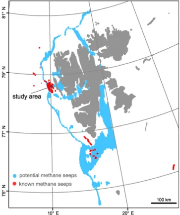
Potential CH₄seep locations around Svalbard were determined by MH stability modeling. The MH stability model (CSMHYD program) [Sloan and Koh, 2008] was used taking bottom water temperatures World Ocean Database 2013 [Boyer et al., 2013] and sediment thermal gradients (Global Heat Flow Database) from around Svalbard as input parameters. Locations, where the hydrate stability zone outcrops at the seabed, are considered to be potential CH₄seep locations. These locations were supplemented with all known CH₄seeps [Sahling et al., 2014;Panieri et al., 2015, this work]. The modeled potential methane seep locations and known methane seeps are illustrated in Figure 2 as light blue and red dots, respectively.

In order to estimate CH₄fluxes from the modeled seep area (blue in Figure 2) and identified CH₄seep areas (red in Figure 2), we used three different independent atmospheric models: (1) the Lagrangian particle dis- persion model FLEXPART [Stohl et al., 2005], (2) the global chemical transport model Oslo CTM3 [Søvde et al., 2012;Dalsøren et al., 2016], and (3) a Lagrangian mass balance box model [Karion et al., 2013;O’Shea et al., 2014]. See section S3 for details about models and simulations.

Figure 2.The identified (red) and potential (blue) seep locations around Svalbard as calculated by methane hydrate stability modeling.

Geophysical Research Letters

10.1002/2016GL068999

3. Results and Discussion

3.1. Observations in the Ocean and Atmosphere

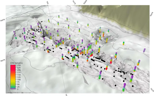
We present the results following the methane migration path from the seafloor through the water column to the lowermost atmosphere close to the sea surface (ship) and higher up usingflight data covering a larger area. Figure 3 illustrates the dissolved CH₄concentrations sampled over the investigated area. Elevated con- centrations were found around the most extended cluster offlares, and the CH₄distribution shows a rapid change at about ~50 m water depth, with the highest dissolved CH₄ concentrations near the seafloor

~150 m depth. Little CH₄is found above the pycnocline (boundary where the density gradient is greatest, affected by temperature and salinity), but sea surface CH₄concentrations are still oversaturated with respect to atmospheric concentrations in a few places eastward, close to the shore

The sea surface CH₄ocean concentrations (Figure 4a) and the atmospheric mixing ratio measured by both the ship (Figure 4b) and the aircraft (Figure 4c) show very similar patterns. In the surface water CH₄was gen- erally<8 nmol L ¹(Figure 4a) with a median of 4.8 nmol L ¹. A maximum of 26 nmol L ¹was found near the shore, where no gasflares are found in the vicinity (Figures 4a and 4b). The elevated surface water CH₄con- centrations coincide with a small increase (<2 ppb) of atmospheric CH₄mixing ratio detected by the ship.

This slightly elevated CH₄close to the shore is probably not due to CH₄released from the seafloor/seeps.

Figure 3 and Figure 4 show that the bottom CH₄concentrations are low in this coastal area. A simultaneous decrease in salinity suggests the intrusion of methane-enriched fresher water [Damm et al., 2005] near the surface increasing the dissolved CH₄concentrations in this particular area.

A 6 km transect was sampled twice in 1 week by the R/VHelmer Hanssento monitor rapid variations of oceano- graphic conditions and their effects on the dissolved CH₄distribution. The maximum bottom water CH₄concen- tration doubled in 1 week from 200 to 400 nmol L ¹(see Figures 4d and S2), while bottom water temperatures remained relatively stable. At the same time, the concentrations above the pycnocline and at sea surface remained relatively stable and low (4–11 nmol L ¹and ~10 nmol L ¹in the surface water on 24 June and 1 July, respectively).

Figure 3.CH₄concentrations from a hydrocast survey offshore of Prins Karls Forland. Thefirst three bottles were taken 5, 15, and 30 m above the seafloor, and the last three bottles were taken 10, 20, and 30 m below the sea surface. The rest of the samples were spread equally in the water column depending on the bottom depth. CH₄concentrations in the ocean are illustrated by colored dots (scale on the bottom left in nmol L ¹). Black dots indicate the location of the gasflares.

Isobaths are from International Bathymetric Chart of the Arctic Ocean version 3 grid and the superimposed higher resolution bathymetry is from the multibeam survey performed during the R/VHelmer Hanssencruise; data were recorded over the period 25 June to 1 July 2014.

This is in agreement with changes reported bySteinle et al. [2015] for bottom water and sea surface water. This change in concentration can be explained either by slower advection during the later observations or that the water was previously CH₄enriched by an emission burst from one or several nearby seep sites. Gas bubble dis- solution modeling from a previous study in the deeper area to the west of our study area estimated that 80% of the bubble-released CH₄is dissolved below the summer pycnocline, and the remaining CH₄is transported northward where it is most likely oxidized by methanotrophic bacteria [Gentz et al., 2014;Steinle et al., 2015].

A similar conclusion came from a box modeling result of dissolved CH₄indicating that ~60% of CH₄released at the seafloor becomes already oxidized before it reaches the overlying surface waters [Graves et al., 2015].

Although our single beam echo sounder studies show bubbles reaching the sea surface, very little CH₄remains in such bubbles by the time they reach the surface [Greinert and McGinnis, 2009].

We compared data from the R/VHelmer Hanssento those from the Zeppelin Observatory for the period from 20 June to 1 August. The CH₄mixing ratio measured aboard the ship during the measurements off Prins Karls Forland agrees well with those recorded by the Zeppelin Observatory, as does the isotopic ratio (see support- ing information Figure S3). Our measurements above theflares were not influenced by long-range transport of methane-enhanced air masses from lower latitudes, as this would have produced noticeable transient enhancements in CH₄, as exemplified in Figure S3.

3.2. Flux Estimates From Ocean to Atmosphere in the Svalbard Region During Summer

We estimate the median ocean-atmosphere CH₄flux based on observations in the ocean, in addition to three top-down constrains of theflux employing three independent models and the atmospheric measurements.

Figure 4.Comparison of CH₄variations in the ocean and atmosphere west of Svalbard and corresponding CH₄flux to the atmosphere. (a) Contour plot of near-surface CH₄ concentration (color scale) at ~10 m depth in the water column. CH₄was measured by oceanographic conductivity-temperature-depth (CTD) stations (crosses) west of Prins Karls Forland (PKF). Observedflares are shown by pink markers. (b) Contour plot of atmospheric CH₄mixing ratio in parts per billion measured aboard R/VHelmer Hanssen (color scale). Ship track is shown by black line;flares are shown by pink markers. (c) CH₄measured by the FAAM aircraft;flares are shown by pink markers. (d) CH₄con- centration in the water column along a transect of CTD stations taken on 1 July 2014 showing a clear stratification of water masses with the pycnocline near 50 m water depth. Density is shown as black contours. (The transect location offshore of Prins Karls Forland is shown in Figure S2b). (e) CH₄flux to the atmosphere at each CTD location as a function of ocean CH₄concentration according to a diffusive model (green points). Flux previously modeled off Northern Siberia during stormy weather [Shakhova et al., 2014] is given by the grey point. Dashed lines show the modelflux at different isotachs (lines of constant wind speed), assuming constant salinity and temperature (averaged over the sampling period used). Horizontal lines show the maximum possibleflux constrained by the atmospheric measurements from the ship, according to FLEXPART and Oslo CTM3 models. FLEXPART and CTM constraints are for the atmospheric sampling period 20 June to 1 August and will vary with weather patterns.

Geophysical Research Letters

10.1002/2016GL068999

We estimate a median ocean-atmosphere CH₄ flux of 0.04 nmol m ²s ¹ (σ= 0.13) from data at each conductivity-temperature-depth (CTD) station using an ocean-atmosphere gas exchange function [Wanninkhof et al., 2009] (Figure 4e). The maximumflux at the CTD stations is 0.8 nmol m ²s ¹which occurred when both dissolved CH₄concentrations and wind speeds were high, 25 nmol L ¹and 9 m s ¹respectively. This model only considers air-sea exchange via diffusion of dissolved CH₄and not the contribution of bubbles of gas reaching the surface. Figure 4e) shows the estimatedflux at different wind speeds, assuming constant salinity and tempera- ture (average from the campaign). Wind speed has a large effect: an increase from 5 to 10 m s ¹increases the modeledflux by almost an order of magnitude. The atmospheric CH₄air mixing ratios aboard the R/VHelmer Hanssenand atZeppelinbefore, during, and after the ship-based measurements off Prins Karls Forland were very similar, with small variations (Figure S3). Hence, the CH₄air mixing ratios above active seep areas were represen- tative of wider regional atmospheric concentrations, with no elevated levels or transient large increases.

To complement our observational-basedflux estimates of dissolved CH₄, we employed three independent atmospheric models to provide top-down constraints of the ocean-atmosphereflux, given the atmospheric concentrations sampled by the aircraft and the ship. This approach also takes potential CH₄from bubbles into account. We only detected a weak increase of 2 ppb in the atmospheric mixing ratio at the ship location close to bubbles, reflecting the potential enhancement from both dissolved CH₄and CH₄from bubbles. We calculated, using a Lagrangian transport model (FLEXPART), the CH₄enhancements at the ship for all locations that would result from a 1 nmol m ²s ¹flux from the area, encompassing the identified and the potential CH₄seep sites around Svalbard [Sahling et al., 2014] (Figure 2). Running FLEXPART backward in time for all ship positions over the period 20 June to 1 August, the modeled CH₄enhancement is shown as the yellow line in the supporting information section, Figure S4; compared to the observations, no correlation (r²= 0.003) is evident. The most sensitive days are the highest 20% modeled peaks (bold yellow line). Using the most sensitive days from this period, we estimate a top-down constraint on theflux from the seep areas of<2.4 ± 1.3 nmol m ²s ¹. This esti- mation assumes that all of the measured 2 ppb variation in the atmosphere is solely due to aflux from the mod- eled seep areas around Svalbard (Figure 2). Similarly, using a forward chemistry transport model (Oslo CTM3) [Søvde et al., 2012], aflux of 3.8 ± 0.7 nmol m ²s ¹was necessary to reproduce the 2 ppb increase in CH₄at the ship, assuming the same emission region shown in Figure 2. This is equivalent to an annual emission of only 0.06 Tg for a constantflux throughout the year, very small compared to the total global annual emission of

~600 Tg of CH₄[Kirschke et al., 2013]. In addition, we used the aircraft measurements to provide another inde- pendent constrain on the maximum possible CH₄flux in the region. The aircraftflew transects below 100 m alti- tude upwind and downwind of the potential seep sites but observed no statistically significant change in CH₄ during these low-levelflights; see Figure 1d for altitudes. A Lagrangian mass balance calculation (similar to that employed byO’Shea et al. [2014] leads to an estimatedflux of 3.0 ± 17.1 nmol m ²s ¹. An estimated upper limit on the ocean-to-atmosphere CH₄flux averaged over the grey shaded area shown in Figure 1d can then be quantified by the mean + 1σvalue of 14.1 nmol m ²s ¹. This represents the maximum possibleflux for this area consistent with the aircraft CH₄measurements and associated uncertainties.

FAAM aircraft measurements were also made in the same location off Prins Karls Forland in a previous Methane in the Arctic Measurement and Modelling (MAMM) campaign in summer 2012 as part of the UK Table 1. Ocean to Atmosphere CH₄Flux Constraints Offshore Prins Karls Forland From Different Independent Methodologies^a

Methodology

Maximum Flux Possible Constrained by the Atmospheric Observations (nmol m ²s ¹)

FLEXPART^btop-down backward modeling 2.4 ± 1.4

Oslo CTM3^ctop-down forward modeling 3.8 ± 1.4

Lagrangian mass balancing—FAAM)^d, top down, exploring upwind/

downwind variations

14.1

aThe potentialflux region is shown in Figure 2 and employing atmospheric observation fromZeppelinandHelmer Hanssenover the period 20 June to 1 August 2014.

bLagrangian particle dispersion model [Stohl et al., 2005;Thompson and Stohl, 2014].

cChemical transport model [Søvde et al., 2012;Dalsøren et al., 2016].

dLagrangian mass balance approach [Karion et al., 2013;O’Shea et al., 2014]. Note that theflux constrain based on the flight data is weaker; there was no statistically significant change in downwind CH₄mixing ratio relative to the measured upwind background, and this is the maximum possibleflux that is consistent with the atmosphericflight measurements and associated uncertainties.

Methane in the Arctic Measurement and Modelling (MAMM) project (seeAllen et al. [2014] for details).

Similarly, any emission from the seep areas was not detectable among the other signals in the aircraft data.

Forward calculations, with a different dispersion model, led to very similar conclusions to those of 2014: that an emissionflux of a few tens of nmol m ²s ¹would have been required to detect the emission in the air- craft data [M. Cain, personal communication, 2016].

In sharp contrast to theflux calculations from the measurement-led approaches discussed here (Table 1), the flux reported byShakhova et al. [2014] from the East Siberian Arctic Shelf is more than 2 orders of magnitude larger, 70–450 nmol m ²s ¹under windy conditions than our measurement-derived maximum for the per- iod. Figure 4e includes a comparison. Part of this large difference can be explained by both higher dissolved CH₄concentrations in surface waters reported in the Siberian area (up to ~400 nmol L ¹) and the higher wind speeds reported byShakhova et al. [2014]. Table 1 compiles our estimates of the spatially averaged maximal flux in the region, as constrained by the atmospheric observations.

4. Conclusion

Despite the obvious influence of seeps on dissolved CH₄concentrations in the ocean west of Svalbard in June– July summer 2014, very little CH₄reaches the atmosphere, neither as bubbles transported nor dissolved gas.

The median wind speed was 6.6 m s ¹during our campaign, and the pycnocline remained stable. We suggest that dissolved methane captured below the pycnocline may only be released to the atmosphere when physical processes remove this dynamic barrier. In such a situation, dissolved CH₄concentrations would rapidly decrease and any largeflux would most likely be transient. Consequently, we conclude that large CH₄releases to the atmosphere with strong impact on the atmospheric levels from subsea sources, including hydrates, do not occur to the west of Svalbard, presently. Shorter periods with largefluxes, particularly during other times of the year such as during ice break-up or storm events, might occur. The role of the pycnocline in this context will be investigated in more detail during long-term ocean observatory recordings in the future.

References

Allen, G., et al. (2011), South East Pacific atmospheric composition and variability sampled along 20°S during VOCALS-REx,Atmos. Chem.

Phys.,11, 5237–5262, doi:10.5194/acp-11-5237-2011.

Allen, G., et al. (2014), Atmospheric composition and thermodynamic retrievals from the ARIES airborne TIR-FTS system—Part 2: Validation and results from aircraft campaigns,Atmos. Meas. Tech.,7, 4401–4416, doi:10.5194/amt-7-4401-2014.

Archer, D. (2007), Methane hydrate stability and anthropogenic climate change,Biogeosciences,4, 521–544.

Berchet, A., et al. (2016), Atmospheric constraints on the methane emissions from the East Siberian Shelf,Atmos. Chem. Phys.,16, 4147–4157, doi:10.5194/acp-16-4147-2016.

Biastoch, A., et al. (2011), Rising Arctic Ocean temperatures because gas hydrate destabilization and ocean acidification,Geophys. Res. Lett., 38, L08602, doi:10.1029/2011GL047222.

Boyer, T. P., et al. (2013),World Ocean Database 2013, NOAA Atlas NESDIS 72, edited by S. Levitus, and A. Mishonov, 2019 pp., Tech. Ed., Silver Spring, Md., doi:10.7289/V5NZ85MT.

Ciais, P., et al. (2013), Carbon and other biogeochemical cycles, inClimate Change 2013—The Physical Science Basis. Contribution of Working Group I to the Fifth Assessment Report of the Intergovernmental Panel on Climate Change, edited by T. F. Stocker et al., pp. 465–570, Cambridge Univ. Press, Cambridge, U. K., and New York.

Collins, M., et al. (2013), Long-term climate change: Projections, commitments and irreversibility, inClimate Change 2013—The Physical Science Basis. Contribution of Working Group I to the Fifth Assessment Report of the Intergovernmental Panel on Climate Change, edited by T. F. Stocker et al., pp. 1029–1136, Cambridge Univ. Press, Cambridge, U. K., and New York.

Dalsøren, S. B., C. L. Myhre, G. Myhre, A. J. Gomez-Pelaez, O. A. Søvde, I. S. A. Isaksen, R. F. Weiss, and C. M. Harth (2016), Atmospheric methane evolution the last 40 years,Atmos. Chem. Phys.,16, 3099–3126, doi:10.5194/acp-16-3099-2016.

Damm, E., A. Mackensen, G. Budeus, E. Faber, and C. Hanfland (2005), Pathways of methane in seawater: Plume spreading in an Arctic shelf environment (SW-Spitsbergen),Cont. Shelf Res.,25, 1433–1452.

Ferré, B., J. Mienert, and T. Feseker (2012), Ocean temperature variability for the past 60 years on the Norwegian-Svalbard margin influences gas hydrate stability on human time scales,J. Geophys. Res.,117, C10017, doi:10.1029/2012JC008300.

Fisher, R. E., et al. (2011), Arctic methane sources: Isotopic evidence for atmospheric inputs,Geophys. Res. Lett.,38, L21803, doi:10.1029/2011GL049319.

Gentz, T., E. Damm, J. S. von Deimling, S. Mau, D. F. McGinnis, and M. Schlüter (2014), A water column study of methane around gasflares located at the West Spitsbergen continental margin,Cont. Shelf Res.,72, 107–118.

Graves, C. A., L. Steinle, G. Rehder, H. Niemann, D. P. Connelly, D. Lowry, R. E. Fisher, A. W. Stott, H. Sahling, and R. H. James (2015), Fluxes and fate of dissolved methane released at the seafloor at the landward limit of the gas hydrate stability zone offshore western Svalbard, J. Geophys. Res. Oceans,120, 6185–6201, doi:10.1002/2015JC011084.

Greinert, J., and D. F. McGinnis (2009), Single bubble dissolution model—The graphical user interface SiBu-GUI,Environ. Modell. Software,24, 1012–1013.

Isaksen, I. S. A., M. Gauss, G. Myhre, K. M. Walter Anthony, and C. Ruppel (2011), Strong atmospheric chemistry feedback to climate warming from Arctic methane emission,Global Biogeochem. Cycles,25, GB2002, doi:10.1029/2010GB003845.

Karion, A., et al. (2013), Methane emissions estimate from airborne measurements over a western United States natural gasfield,Geophys.

Res. Lett.,40, 4393–4397, doi:10.1002/grl.50811.

Geophysical Research Letters

10.1002/2016GL068999

Acknowledgments

The project MOCA—Methane Emissions from the Arctic OCean to the Atmosphere:

Present and Future Climate Effectsis funded by the Research Council of Norway, grant 225814. CAGE—Centre for Arctic Gas Hydrate, Environment and Climate research work was supported by the Research Council of Norway through its Centres of Excellence fund- ing scheme grant 223259. Nordic Center of Excellence eSTICC (eScience Tool for Investigating Climate Change in north- ern high latitudes) is funded by Nordforsk, grant 57001. Additional support from the Natural Environment Research Council MAMM project (grant NE/I029293/1) and the ERC though the ACCI project, project 267760.

Kirschke, S., et al. (2013), Three decades of global methane sources and sinks,Nat. Geosci.,6, 813–823.

Knies, J., E. Damm, J. Gutt, U. Mann, and L. Pinturier (2004), Near-surface hydrocarbon anomalies in shelf sediments off Spitsbergen:

Evidences for past seepages,Geochem. Geophys. Geosyst.,5, Q06003, doi:10.1029/2003GC000687.

Myhre, G., et al. (2013), Anthropogenic and natural radiative forcing, inClimate Change 2013—The Physical Science Basis. Contribution of Working Group I to the Fifth Assessment Report of the Intergovernmental Panel on Climate Change, edited by T. F. Stocker et al., pp. 659–740 , Cambridge Univ. Press, Cambridge, U. K., and New York.

Nisbet, E. G., E. J. Dlugokencky, and P. Bousquet (2014), Methane on the rise—Again,Science,343, 493–495.

Nordli, Ø., R. Przybylak, A. E. J. Ogilvie, and K. Isaksen (2014), Long-term temperature trends and variability on Svalbard: The extended Svalbard Airport temperature series, 1898–2012,Polar Res.,33, 21349, doi:10.3402/polar.v33.21349.

O’Shea, S. J., G. Allen, Z. L. Fleming, S. J.-B. Bauguitte, C. J. Percival, M. W. Gallagher, J. Lee, C. Helfter, and E. Nemitz (2014), Areafluxes of carbon dioxide, methane, and carbon monoxide derived from airborne measurements around Greater London: A case study during summer 2012,J. Geophys. Res. Atmos.,119, 4940–4952, doi:10.1002/2013JD021269.

O’Shea, S. J., S. J.-B. Bauguitte, M. W. Gallagher, D. Lowry, and C. J. Percival (2013), Development of a cavity-enhanced absorption spectro- meter for airborne measurements of CH4and CO2,Atmos. Meas. Tech.,6, 1095–1109.

Panieri, G., et al. (2015), Gas hydrate deposits and methane seepages offshore western Svalbard and StorfjordrennaBiogeochem. Biol. Invest.

CAGE15-2 Cruise Rep.

Panieri, G., C. A. Graves, and R. H. James (2016), Paleo-methane emissions recorded in foraminifera near the landward limit of the gas hydrate stability zone offshore western Svalbard. G3,Geochem. Geophys. Geosyst.,17, 521–537, doi:10.1002/2015GC006153.

Pitt, J. R., et al. (2016), The development and evaluation of airborne in situ N2O and CH4sampling using a Quantum Cascade Laser Absorption Spectrometer (QCLAS),Atmos. Meas. Tech.,9, 63–77.

Portnov, A., A. J. Smith, J. Mienert, G. Cherkashov, P. Rekant, P. Semenov, P. Serov, and B. Vanshtein (2013), Offshore permafrost decay and massive seabed methane escape in water depths>20 m at the South Kara Sea shelf,Geophys. Res. Lett.,40, 3962–3967, doi:10.1002/

grl.50735.

Portnov, A., S. Vadakkepuliyambatta, J. Mienert, and A. Hubbard (2016), Ice-sheet driven methane storage and release in the Arctic,Nat.

Commun.,7, 10314, doi:10.1038/ncomms10314.

Rajan, A., J. Mienert, and S. Bünz (2012), Acoustic evidence for a gas migration and release system in Arctic glaciated continental margins offshore NW-Svalbard,Mar. Petrol. Geol.,32, 36–49.

Ruppel, C. D. (2011), Methane hydrates and contemporary climate change,Nat. Educ. Knowl.,3(10), 29. [Available at http://www.nature.com/

scitable/knowledge/library/methane-hydrates-and-contemporary-climate-change-24314790.]

Sahling, H., et al. (2014), Gas emissions at the continental margin west of Svalbard: Mapping, sampling, and quantification,Biogeosciences,11, 6029–6046.

Shakhova, N., I. Semiletov, I. Leifer, A. Salyuk, P. Rekant, and D. Kosmach (2010), Geochemical and geophysical evidence of methane release over the East Siberian Arctic Shelf,J. Geophys. Res.,115, C08007, doi:10.1029/2009JC005602.

Shakhova, N., et al. (2014), Ebullition and storm-induced methane release from the East Siberian Arctic Shelf,Nat. Geosci.,7, 64–70.

Sloan, E. D., and C. A. Koh (2008),Clathrate Hydrates of Natural Gases, 3rd ed., CRC Press, Boca Raton, Fla.

Smith, A. J., J. Mienert, S. Bünz, and J. Greinert (2014), Thermogenic methane injection via bubble transport into the upper Arctic Ocean from the hydrate-charged Vestnesa Ridge, Svalbard,Geochem. Geophys. Geosyst.,15, 1945–1959, doi:10.1002/2013GC005179.

Søvde, O. A., M. J. Prather, I. S. A. Isaksen, T. K. Berntsen, F. Stordal, X. Zhu, C. D. Holmes, and J. Hsu (2012), The chemical transport model Oslo CTM3,Geosci. Model Dev.,5, 1441–1469.

Steinle, L., et al. (2015), Water column methanotrophy controlled by a rapid oceanographic switch,Nat. Geosci.,8, 378–382.

Stohl, A., C. Forster, A. Frank, P. Seibert, and G. Wotawa (2005), Technical note: The Lagrangian particle dispersion model FLEXPART version 6.2,Atmos. Chem. Phys.,5, 2461–2474.

Thompson, R. L., and A. Stohl (2014), FLEXINVERT: An atmospheric Bayesian inversion framework for determining surfacefluxes of trace species using an optimized grid,Geosci. Model Dev.,7, 2223–2242.

Veloso, M., J. Greinert, J. Mienert, and M. De Batist (2015), A new methodology for quantifying bubbleflow rates in deep water using split beam echo sounder: Examples form the Arctic offshore NW Svalbard,Limnol. Oceanogr.: Methods,13, 267–287, doi:10.1002/lom3.10024.

Wanninkhof, R., W. E. Asher, D. T. Ho, C. Sweeney, and W. R. McGillis (2009), Advances in quantifying air-sea gas exchange and environmental forcing,Annu. Rev. Mar. Sci.,1, 213–244.

Westbrook, G. K., et al. (2009), Escape of methane gas from the seabed along the West Spitsbergen continental margin,Geophys. Res. Lett.,36, L15608, doi:10.1029/2009GL039191.