Research Collection
Working Paper
More Laws, More Growth? Evidence from U.S. States
Author(s):
Ash, Elliott; Morelli, Massimo; Vannoni, Matia Publication Date:
2020-10
Permanent Link:
https://doi.org/10.3929/ethz-b-000454202
Rights / License:
In Copyright - Non-Commercial Use Permitted
This page was generated automatically upon download from the ETH Zurich Research Collection. For more information please consult the Terms of use.
Center for Law & Economics Working Paper Series
Number 15/2020
More Laws, More Growth?
Evidence from U.S. States
Elliott Ash
Massimo Morelli Matia Vannoni
October 2020
All Center for Law & Economics Working Papers are available at
More Laws, More Growth?
Evidence from U.S. States
Elliott Ash, Massimo Morelli, Matia Vannoni
∗October 22, 2020
Abstract
This paper analyzes the conditions under which more detailed legislation con- tributes to economic growth. In the context of U.S. states, we apply natural language processing tools to measure legislative flows for the years 1965-2012.
We implement a novel shift-share design for text data, where the instrument for legislation is leave-one-out legal-topic flows interacted with pre-treatment legal- topic shares. We find that at the margin, higher legislative detail causes more economic growth. Motivated by an incomplete-contracts model of legislative de- tail, we test and find that the effect is driven by contingent clauses, that the effect is concave in the pre-existing level of detail, and that the effect size is increasing with economic policy uncertainty.
∗Elliott Ash, ETH Zurich, ashe@ethz.ch; Massimo Morelli, Bocconi University and CEPR, mas- simo.morelli@unibocconi.it; Matia Vannoni, King’s College London, matia.vannoni@kcl.ac.uk. We acknowledge financial support from the European Research Council Advanced Grant 694583. We thank Massimo Anelli, Pierpaolo Battigalli, Kirill Borusyak, Quentin Gallea, Livio di Lonardo, Xavier Jaravel, Giovanni Maggi, and Piero Stanig for helpful comments. We also wish to thank seminar participants at the Fifth Columbia Political Economy Conference, ETH Political Economy Workshop, QPE Brown Bag Seminar at King’s College London, and Stockholm School of Economics Seminar for helpful comments. We thank David Cai, Claudia Marangon, and Emiliano Rinaldi for helpful research assistance.
Figure 1: State GDP and Legislative Detail, 1966 and 2012
A) State GDP vs. Detail, 1966 (B) State GDP vs. Detail, 2012
Slope = .24***
(s.e. = .09)
14 16 18 20 22
Log GSP
7 8 9 10 11
Log Provisions
Log GSP Fitted values
Slope = .44***
(s.e. = .10)
14 16 18 20 22
Log GSP
7 8 9 10 11
Log Provisions
Log GSP Fitted values
Notes. Scatter-plots for the relationship between (log) provisions and (log) state GDP at the beginning of our time period (1966) and the end (2012).
1 Introduction
In the cross section, states with larger, more complex legal systems also tend to have larger, more productive economies. The correlation between statute detail and GDP in U.S. states, illustrated in Figure1 Panels A and B, provides a clear example of this empirical regularity. A key question is whether these correlations reflect causal links.
While a larger economy could lead to more detail mechanically (as, for example, more industries need to be regulated), it could also be that more legislation (if well- designed) could also cause economic growth. Consider the introduction of detailed property rights protections, and establishment of the rule of law (Dam, 2007). These institutions could help markets run more efficiently, encourage investment, and increase growth. On the other hand, excessive regulation could hinder economic growth (Niska- nen, 1971, Botero et al., 2004). Hence, even in an ideal world of benevolent legislators, one could postulate the existence of an optimal level of regulatory complexity given the current state of the economy, where moving toward the optimum from either side would increase growth.
Taking inspiration from the literature on endogenously incomplete contracts, this paper offers a set of predictions about when and where the marginal increments in legislative detail can have positive effects on growth. Theoretically, we view legislation drafting as contract writing by a benevolent principal, who has to choose the level of completeness given the marginal benefit and the writing costs. The main prediction of the theory based on Battigalli and Maggi (2002, 2008) framework is that when legislative
details on an issue or sector increase through an increase in contingent clauses, then the effects of such an increase in legislative details is positive for growth. Second, the model predicts that the effect should be concave, in the sense that legislation would have a larger effect starting from a low-detail baseline. Third, the effect is predicted to be larger when there is higher economic uncertainty (and hence more contingencies are needed).
We take these predictions to data in the context of legislation and economic output in U.S. states for the years 1965 through 2012. For each state and biennium, we produce a measure of legislative detail from the text of state laws. The measure draws on recently developed methods in computational linguistics to detect legally relevant requirements from legislation (Vannoni et al., 2019), extracting more signal than coarser measures based on word or character counts. Further, we use a topic model to measure the allocation of provisions across legal categories (Blei et al., 2003).
Our empirical strategy is a shift-share instrumental variables design, based on Bar- tik (1994), that isolates exogenous variation in legislative detail. Analogous with stan- dard shift-share instruments that use sector-specific economic flows interacted with pre-treatment sector shares, we construct our instrument using topic-specific legislative flows interacted with pre-treatment topic shares. The exclusion restriction is based on the orthogonality of shifters: we assume that common (e.g. technological) factors across states drive them to legislate on a topic and these factors are unrelated to economic growth. In other words, we assume that topic-specific legislative flows are exogenous, in line with recent econometric work by Borusyak and Jaravel (2017) and Adao et al.
(2019). Our design passes a number of checks recently developed by econometricians for probing the exogeneity of shift-share instruments (Goldsmith-Pinkham et al., 2020, Borusyak and Jaravel, 2017, Adao et al., 2019).
Our main result is that more state-level legislation tends to boost the state economy.
This effect is robust to a range of alternative specifications and inclusion of covariates.
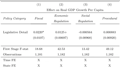
The growth effect is reflected in both increased wages and increased profits. The effect is driven by fiscal and regulatory policy, rather than by social policy (e.g. crime) or procedural issues (e.g. electoral districting).
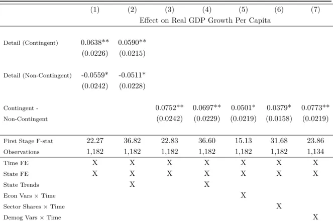
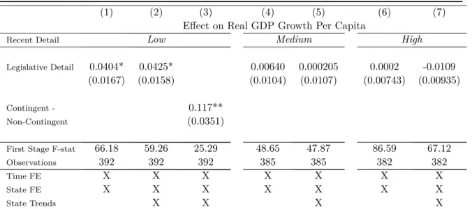
Next we test some of the more subtle predictions of the model. First, we find that the effect of detail on growth is driven by contingent clauses (those containing “if”,
“except”, etc.). Second, we find that the effect is stronger for states with a low-detail (low-regulation) baseline (the concavity effect). Third, we extend the approach of Baker et al. (2016) to local newspapers to produce a measure of economic policy uncertainty
by state over time. The effect of detail – and in particular contingent clauses – is stronger during periods of higher economic policy uncertainty.
These results contribute to the centuries-long debate on how government regulation (as opposed to expenditure) is related to the functioning of the economy. One strand of literature – the positive view – stresses that a certain level of regulation is likely needed for the economy to grow (Di Vita, 2017). There is legislation needed to regulate externalities, define the tax base, and allocate government expenditures. Some of the economic literature on tax legislation suggests that more legislation could be better for the economy, to the extent that it reduces legal uncertainty (Slemrod, 2005, Graetz, 2007). In this sense, incomplete laws can be understood as incomplete social contracts (Weisbach, 2002, Holtzblatt and McCubbin, 2003, Givati, 2009).
On the other hand, the negative view of public choice theory holds that excessive regulation could hinder economic growth (Niskanen, 1971). The main argument is that regulation deters growth by hindering new firm formation, competition, and innovation (Fonseca et al., 2001, Nicoletti and Scarpetta, 2003, Ciccone and Papaioannou, 2007).
There are also indirect costs, by disincentivising people to acquire skills (Ciccone and Papaioannou, 2007). Braunerhjelm and Eklund (2014) suggest that the burden of com- plex taxes has a negative effect on market entry. Kawai et al. (2018) show that failing to consider complementarity in reforms (kludges) can have negative effects. Finally, Foarta and Morelli (2020) provide a more nuanced theoretical explanation identifying conditions under which higher detail could be either good or bad for the economy.
Perhaps reflecting the mixed theoretical results, the empirical literature is also mixed. On the one side, there are a set of papers documenting a positive correla- tion between legislative detail and growth. For example, Mulligan and Shleifer (2005) show that population is positively related to the detail of legislation in U.S. states (as measured by number of pages). In Japan, Fukumoto (2008) finds that economic growth is associated with higher volume of legislation over time. Kirchner (2012) finds a similar effect for Australia. These papers cannot make strong causal claims, however.
On the other side, a number of papers find some evidence for the negative view.
Botero et al. (2004) show in a cross-country c9omparison that regulation of labor is associated with lower labor force participation and higher unemployment. Similarly, Campbell et al. (2010) argue that regulation often does not provide efficient solutions to conflicts and, therefore, does not foster economic development. In a comparison between Italian regions, Di Vita (2017) finds that regulatory complexity is related to lower economic growth and per capita income. Also in Italy, Gratton et al. (2018)
suggest that electoral incentives may create excessive reformism and deterioration of the quality of legislation, which negatively impacts economic growth.
Our paper builds on this literature in a number of ways. First, we leverage text as data in a new way, employing a linguistically motivated measure of legal detail rather than simple word counts or page counts. Second, we use exogenous variation in legislative detail, so that our estimates have a causal interpretation. Third, we test a set of more subtle theoretical predictions that provide support for an incomplete contracts model of legislating, in particular highlighting the importance of contingency and economic uncertainty.
The paper is organized as follows: Section 2explains how the theory of endogenous incomplete contracts generates the four main hypotheses that we test in this paper.
Sections3, 4, and 5 describe the data, text analysis methods, and empirical approach, respectively. Section 6 reports the main results and robustness checks on detail and growth, while Section7explores the more subtle theoretical predictions on contingency, concavity, and uncertainty. Section8 concludes.
2 Legislating as Incomplete Contracting
In this section we describe how the writing costs approach of Battigalli and Maggi (2002, 2008) can be adapted to the legislative process in order to derive a set of hypotheses on the causes and consequences of legislative detail. We start by using the logic of Battigalli and Maggi (2002) to describe the law as an incomplete contract; we will then describe how some insights can also be derived from Battigalli and Maggi (2008), where the focus is not on the degree of completeness of a law but on the type of clauses (contingent or spot) and on their evolution over time. We will derive from this framework a set of hypotheses that can be tested using our proposed methodology.
2.1 What can we learn from the writing costs approach
A law can be viewed as an incomplete contract between the legislator (the principal) and the citizens (agents), with an efficiency objective. Incompleteness can take the form of rigidity (non-contingent clauses) or discretion (empty clauses). The optimal degree of incompleteness depends on writing costs, that could be the following: the cost of figuring out the relevant contingencies and obligations, the cost of thinking how to describe them, the cost of time needed to write the law. Thus these are all costs
related to the details and precision of the language of the law.
The language of the law consists of primitive sentences that describe (1) elementary events and (2) elementary actions, plus logical connectives (e.g., “not,” “and,” “or”).
This language can be used to describe state- dependent constraints on behavior, or in other words, a correspondence from states to allowable behaviors. Each primitive sentence has a cost and the total cost of writing the contract is a function of the costs of its primitive sentences about events and actions . It follows naturally that contingent clauses are more costly than non-contingent clauses.
A contingency is a formula about the environment, i.e., could include different events with different logical connectives, so a contingency could be event 1 or event 2, and another contingency could be event 1 and 3. An instruction is a formula of behavior, i.e. a set of actions with some logical connectives, like take action 1 and or 2.1 Omitting from the text of a law an elementary sentence about the possible events or situations that could occur saves on the cost of describing contingencies, but makes the contract rigid. Omitting from the contract an elementary action saves on the cost of describing behavior, but gives discretion to the agent.
Adjusting Battigalli and Maggi (2002) main characterization result about the opti- mal contract to our context, we can informally restate their proposition 1 saying that an optimal law should have contingent clauses for the most important decisions regulated by such a law, while less important decisions can be regulated by rigid or non-contingent clauses and the least important decisions can be left to discretion.
In more uncertain environments the optimal law (proposition 2(II) in Battigalli and Maggi (2002)) contains more contingent clauses, fewer rigid clauses, and leaves more discretion to the agent. This is intuitive: when uncertainty is higher the efficiency cost of ignoring low-probability events and writing rigid clauses is higher, hence the number of rigid clauses is lower. Moreover, when uncertainty is higher, both contingent clauses and missing clauses increase in number.
While in the above summary of the static Battigalli and Maggi (2002) model the states of the world without a precise instruction are described as cases of agents’ discre- tion, Battigalli and Maggi (2008) allow such discretion cases to be regulated by informal contracts or spot clauses – this becomes a possibility because of repeated play.
1An important assumption in the framework in Battigalli and Maggi (2002) is that the language just described is common-knowledge for the parties and the courts, and hence states of the world and actions are perfectly verifiable by courts. This ensures that there are no problems of ambiguous interpretation of the law in this efficiency framework.
When the cost of describing contingencies is low relative to the cost of (re-)negotiating actions after each unregulated contingency, then contingent clauses are optimal to be- gin with; a spot approach is optimal when this relative cost is high; and an enrichment approach (where when a new unregulated contingency occurs it induces an enrichment of the contingent clauses in the law) may be optimal when this relative cost takes intermediate values.
2.2 Deriving testable predictions
In this section we use the framework described above to derive a set of testable predic- tions.
Completeness. The first aggregate prediction coming out of the optimal contract framework is that if more legislative details are added by a benevolent principal, it must be because they are beneficial in the context where they are added. In other words:2
H0: Given the benevolence assumption on legislators, the greater the complete- ness of law, the better the economic outcomes to be expected – the completeness hypothesis.
Contingency. The second prediction that we can derive from the Battigalli and Maggi (2002, 2008) framework related to contingent clauses. Suppose that for each issue or topic there are plenty of contingencies that one could potentially differentiate, but each contingency requires a constant marginal writing cost. Even if the marginal writing cost of an extra contingency is constant, the marginal benefit depends on many things that could vary a lot from state to state and from year to year, as well as some common component that relates to technological changes or other exogenous transfor- mations of the topic to be regulated.3 As a result, given a fixed marginal writing cost
2Given benevolence and rationality of the designer, in contract theory we take it for granted that in the absence of costs of describing contingencies, a complete contract specifying what would happen in all possible realizations of the states of the world would be better than leaving the contract incomplete (Dye, 1985).
3For example, in a state where all employees are in one or two sectors without many differentiations of skills, the marginal benefit from new contingent statements related to different sectors, seniority, education or other observables would be low. Hence, that state might have relatively simple labor laws and tax laws with non-contingent statements. On the other hand, in a state where skill differentiation
but wide variation in the benefit function, the state legislators choose different levels of contingent legislative detail across states.
The optimal level of completeness of contracts is increasing in the marginal benefit of adding contingencies. Hence we should expect the relation between contingent clauses and growth to be stronger than for other clauses. That is, clauses along these lines: “if a worker has such characteristics... then a firm with such other characteristics could employ him or her with a special tax treatment, transfer, labor law relaxation, etc...”
should be expected to have a positive effect given that it is more costly to write and hence a rational legislator who has decided to introduce it must have anticipated a high marginal benefit from it. The testable hypothesis that corresponds to this reasoning is:
H1: The changes in legislative detail that most affect the growth prospects of a state are additional contingent clauses – thecontingency hypothesis.
If at some point in time comes a shock such as the advent of internet and new exogenous elementary events and actions arise, the existing legislation is not optimal to maximize the surplus. As a result, legislators write more clauses (as we have more events and actions) and more specifically write more contingent clauses (as there are more combinations). Now clauses like: “if there is good internet connection, the worker shall work from home” could be added and be beneficial. We expect that contingent statements to matter most for economic performance. A side prediction would be that contingent clauses would be even more beneficial in states with greater economic complexity – more sectors, more levels, more segmentation, more strategic incentives to be given, etc.
Concavity. We now turn to a third implication of the Battigalli and Maggi (2002) framework. Assume for simplicity that each contingent clause has the same cost c.
Thus, a law that includes l contingent clauses has cost cl. The state j’s marginal benefit from adding a contingent clause is a function B(l, t, wj), where t ∈ R+ is a parameter capturing a common factor (like technological change) andwj ∈R+is a state specific parameter capturing the degree of complexity of the economy to be regulated in state j. Let ∂B∂t > 0, ∂w∂B
j > 0, and ∂B∂l < 0 (the latter capturing a concavity assumption).4
matters, there is a higher marginal benefit from more clauses as, for example, the planner might find it important to give incentives to workers to switch from one sector to another.
4Note also that in an optimal contracting framework with constant marginal writing cost of con- tingent clauses, such contingent clauses should be added in order of importance -- another source of
A state prescribing a rigid clause to always be at the office from 9 to 5 could be optimal in a statej with a low wj while a state k with a greater wk > wj may display already a contingent clause that working from home is possible when some condition on traffic or weather is met. In other words, state k with high wk may optimally have l∗k > lj∗. Suppose that this is the case at time 0 with common technology t0. Consider an exogenous shock at time 1 determiningt1 > t0 (like the invention of internet), such that l∗k(t1) =lk∗(t0) + 1 and l∗j(t1) =lj∗(t0) + 1.
It follows naturally, given the concavity assumption, that the effects must be bigger in state j. When a change in t makes it convenient for both states to add a contingent clause like “if there is good internet connection, the worker shall work from home” then this addition benefits relatively more state j.
H2: An exogenous increase in legislative completeness will have a greater growth dif- ferential in the states with lower initial level of legislative detail – the concavity hy- pothesis.
Uncertainty. The fourth implication of the Battigalli and Maggi (2002) framework concerns the role of uncertainty. That is, it is plausible that the marginal benefit of contingent clauses is higher in states that are exposed to greater uncertainty. The more uncertain are the relevant situations, the more important should be to account for different possible contingencies as far as important issues are concerned, whereas more discretion could be allowed in low importance issues. The functional form for the marginal benefit of an additional contingent clause could be enriched by adding an additional parameter uj ∈ R+ capturing the degree of uncertainty in state j. The simple hypothesis to be tested is that indeed the marginal benefit of more contingent clauses whenuj is higher is positive.
H3: The greater or the more frequent the sources of uncertainty in a state, the greater will be the growth benefit from higher legislative detail, and especially from more contingent clauses.
We will be able to test this hypothesis only at the state aggregate level, whereas testing it in particular on the high importance issues when such issues suffer from greater uncertainty would require some non trivial agreement on importance ranking, something that we could study in future extensions of this research.
concavity.
Table 1: Summary Statistics
(1) (2) (3) (4) (5)
Variables Obs Mean SD Min Max
Economic Output Variables
Log Real GSP per Capita 1,250 3.652 0.281 2.803 4.844
Log Real GSP 1,250 17.79 1.436 14.09 21.54
Log Real GSP per Capita Growth 1,249 0.031 0.050 -0.174 0.332
Log Real GSP Growth 1,250 0.134 0.070 -0.087 0.665
Log Employment Growth 823 0.057 0.064 -0.151 0.930
Log Number of Establishments Growth 823 0.045 0.058 -0.146 0.409 Log Establishment Profit Growth 550 0.163 0.109 -0.403 0.818 Statute Text Variables
Log Provisions (Legislative Detail) 1,183 9.211 0.887 2.996 11.42 Log Contingent Provisions 1,183 7.528 0.983 0.405 9.859 Log Non-Contingent Provisions 1,183 8.908 0.893 2.890 11.03 Covariates
Log Population 1,250 14.94 1.029 12.51 17.47
Democratic Control 1,127 1.802 1.057 0 3
Log Income 1,250 3.479 0.267 2.563 4.144
Log Govt. Expenditure 1,250 15.57 1.471 11.89 19.46 Log Legis. Expenditure 1,250 9.410 1.384 5.176 12.73
Notes. Summary statistics for the main variables. The different number of observations is due to the availability of different years in the different datasets/sources we use.
3 Data Sources
This section describes the data and provides summary statistics. The variables can be roughly divided into three categories: data on economic output and growth, statute text data and legislative detail, and control variables. The main summary statistics are reported in Table1.
The dataset for our empirical analysis ranges from 1965 through 2012. This period is determined by the beginning of the economic growth variables (in 1965) and the ending of the legislative text variables (in 2012). The data are constructed by biennium (two-year periods), since many states publish their compiled statutes once every two years.
Economic Activity. We have a rich array of variables on the economic conditions by year in each of the 50 states. These data are assembled from the Bureau of Economic Analysis Regional Accounts, County Business Patterns, Klarner (2013), and Ujhelyi (2014).
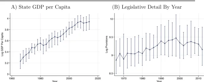
As our empirical analysis looks at how legal flows impact economic growth, the key variable Yst is local growth, measured by the change in log per capita Gross State Product (GSP) in statesbetween yeart−2 and yeart(as the data are at the biennium level). Appendix FigureA.1 shows the evolution of this variable over the time period of the data. The data on the numerator (total real GSP) and the denominator (total population) will also be used separately. All economic variables denominated in dollars are deflated to 2007 values using the state-level CPI.
We have a number of additional measures of economic activity. On the worker side, we have labor income and employment. On the firm side, we have number of establishments and profits.
State Session Laws Corpus. The dataset on legislation includes the full text of U.S.
state session laws. This corpus consists of the statutes enacted by each state legislature during each session. The statutes modify the text in the state’s compiled legislative code. They therefore can include new laws, revisions to existing laws, and repeal of existing laws. As mentioned, the laws are published annually or biennially; to ensure consistency, the dataset is built biennially.
The text from this corpus is produced from optical character recognition (OCR) applied to printed laws. From inspecting samples, the OCR is high quality. Figure 2 shows the scanned copy of a page from a statute enacted in the Texas Legislature for the 1889 session. As can be seen, although the statute is old, the quality of the digitized version is quite good.
Still, as with any historical digitized corpus there are a significant number of OCR errors. At a minimum, OCR errors add measurement error to the legislative detail measure. This is not a major problem for our empirical analysis as long as the OCR error rate is not correlated with either the outcome or the instrument for detail. If it is classical measurement error, it would attenuate estimates. To investigate this, we computed a proxy for OCR as the misspelling rate per word. We found that our instrument is not correlated with the misspelling rate (Appendix FigureA.11).5
5In addition, controlling for OCR error rate in our main results does not change them.
Figure 2: State Session Laws Corpus
Notes. Scanned image and associated OCR for example page from State Session Laws corpus.
Demographics. We link the data on economics and law to demographic data the state level. Besides population, we use census information on the age distribution, the fraction of urban population, and the share of foreign born population.
State government finances. We use a set of data on local government revenues and expenditures from the state government finances census. These include total gov- ernment expenditures (in 1000s current dollars), and legislative expenditures (in 1000s current dollars).
Politics. Next, we use measures of state political conditions. In particular, we have a measure of Democratic Control, which is the number of governing bodies (lower chamber, upper chamber, and governor) controlled by Democrats. This ranges from zero to three.
Local economic uncertainty. Finally, we have information on state-year-level eco- nomic uncertainty constructed from the text of newspaper articles. For this purpose, we use the searchable local newspaper archive newspapers.com, which can programmat- ically provide counts by state and year for articles meeting search criteria. Following
Baker et al. (2016), we count the number of articles mentioning the phrase ‘economic uncertainty’ in a state in a given biennium. We construct a frequency by taking this count divided by the total number of news articles.
4 Text Analysis Methods
This section summarizes our methods for extracting useful measures from the statute texts.
4.1 Measuring Legislative Detail
Using the digitized text of the state session laws, we start by segmenting the text for each biennium into statutes. Roughly speaking, a “statute” is a singular, coherent enacted bill or policy. It usually corresponds to a “chapter” in the compiled legislative code, which is the second level of organization beneath titles. Appendix Figure A.1 Panel A shows the distribution of the number of statutes by biennium. Panel B shows the distribution of the number of words per statute. Panels C and D respectively show the time series for the number of statutes, and number of words per statute, over time.
Next, the statutes are segmented into sentences using a sentence tokenizer. For each sentence, we extract legally relevant statements following the method in Vannoni et al.
(2019) and Ash et al. (2020). The method works as follows, with more detail provided in Appendix B.2.
We apply a syntactic dependency parser to construct data on the grammatical relations among words in each sentence (Dell’Orletta et al., 2012, Montemagni and Venturi, 2013), as illustrated in Appendix FigureA.5. The dependency parse identifies the main verb in a sentence segment, along with the associated subject, object, helping verb, and information on negation.
To extract legally relevant statements, we define a set of legislative provision types (also called legal frames), including obligations, definitions, modifications, and so on (Soria et al., 2007, Saias and Quaresma, 2004). We extract dependency tags associated with each legislative provision type (van Engers et al., 2004, Lame, 2003); for instance, a constraint is characterized by three potential structures: a negative structure with a modal, such as ‘the Agent shall not’; a negative structure with a permission verb, such as ‘the Agent is not allowed’; or a positive structure with a constraint verb, such as ‘the Agent is prohibited from’. The set of provision types, with tagging rules, are listed in
Appendix Table A.2. Vannoni et al. (2019) and Ash et al. (2020) use this method to count provisions across different agent types. Here, the aim is less targeted – we count the number of legal provisions by state and over time.
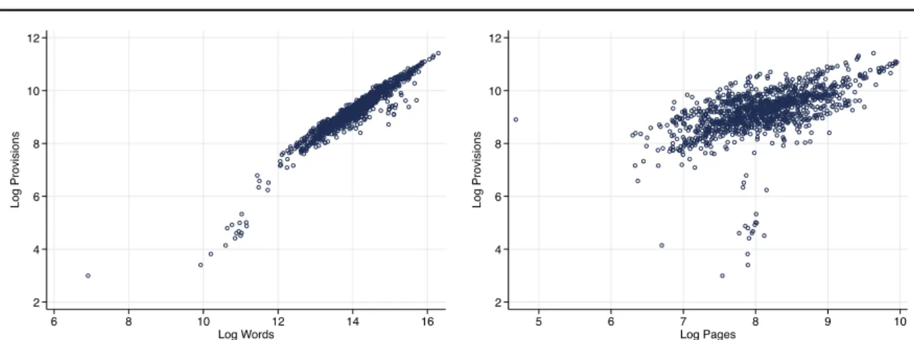
Our measure of legislative detail Wst is the number of legal provisions counted in the session laws for a state at biennium t. To assess proportional changes in detail, we use the log of the counts. The evolution of this measure, by year, is illustrated in FigureA.1. Counting provisions should provide a cleaner measure of the flow of legal requirements than would be obtained by a coarser measure, such as word counts or page counts. The latter type of measure would be noisier because they include a lot of non-legislative or otherwise less informative content. Vannoni et al. (2019) provide some validation against human annotations that our parser-based measure does a better job than simpler measures in identifying legally relevant statements. Appendix Figure A.3 shows that provision counts and word counts are correlated. In Appendix Table A.11we explore variations on our analysis using word counts or page counts.
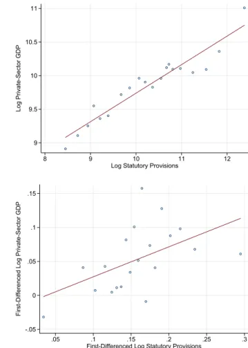
As shown above in Figure 1 and in in the binned scatterplots in Appendix Figure A.2, growth and detail are positively related, both across-states in the cross section and within-state over time. While growth in the economy and growth in laws tend to co-occur, they could do so for many non-causal reasons. Our empirical strategy is designed to address these confounders.
4.2 Allocating Laws to Topics
An essential ingredient in our analysis is to assign statutes to topics. To learn and assign topics, we apply the Latent Dirichlet Allocation (LDA) model described in Blei et al. (2003). This algorithm, by now well known in the literature on text data in political economy (Grimmer and Stewart, 2013, Hansen et al., 2018), assumes that every document is a distribution over topics, which in turn is a distribution over words and phrases. A document is generated by drawing topic shares, and then the words of the document are drawn from those topics.
We trained LDA on our corpus at the statute level using the Mallet wrapper from the Python gensim package. The main tunable hyperparameter in LDA is the number of topicsK. Starting withK = 6 topics, we increased the number by multiples of 6 (12, 18, ..., etc) to find the topic count that maximized the topic coherence score. This score was maximized at K = 42. We also inspected the topics subjectively, and we agreed that the specification with K = 18 topics was a good balance for a relatively small
number of intuitive, coherent topics. After producing our main empirical results for all topic countsK ∈ {6,12, ...,48}, we found that the instrument constructed withK = 18 topics (more details below) generates the most consistent estimate across specifications with different sets of predetermined covariates. Therefore, we have two preferred LDA models: 18 topics and 42 topics. For our main results, however, the topic number choice is not important. In Appendix TableA.10we show consistent results for all LDA models produced (K ∈ {6,12, ...,48}).
The baseline specification for the main text uses the LDA model withK = 18 topics.
The list of 18 topics is reported in Table 2, sorted by most to least frequent in the state session laws corpus. The model produces clearly interpretable topics for vehicle regulation, licensing, courts, project funding, childcare services, trusts and estates, employment law, taxes, land regulation, retirement regulation, etc. These are the types of legal policy areas that one would expect to arise in the business of U.S. state government.
The 42-topic LDA model is mainly used to flesh out our results by policy type. These more granular topics were more easy than the 18-topic model to divide into broader policy areas: economic regulation, fiscal policy, social regulation, and procedural. To make this assignment to policy groups, all three of the co-authors annotated the topics and we assigned the majority annotation, with some discussion under disagreement.
The list of topics, with broader category assignments, is reported in Appendix Table A.3. Appendix FigureA.6shows the legislation shares across these four categories over time.
Beyond these word lists, we further interpret the topics by producing lists of sen- tences that are most distinctive of each topic. Lists of these sentences are provided in Appendix B.3. Overall they are quite intuitive and show that meaningful policy categories are being recovered by LDA.
Using the trained models, we assign to every statute a distribution over topics based on the words and phrases in that statute. For each state-biennium, the number of provisions by topic is computed by the sum of provisions in that state-biennium’s statutes, weighted by the topic share of each statute. Formally, let Lst be the set of laws in states timet. Each statutei∈Lst has a provision countwi and a distribution over topics~v 3vik,∀k ∈ {1, ..., K}, wherevik ≥0 andPkvik= 1. Then define legislative
Table2:ListofTopics,18-TopicSpecification LabelFrequencyMostAssociatedWords Courts0.0724courtjudgmentattorneycaseappealcivilpetitionsherifftrialcircuit_court district_courtsuch_personcomplaintcounselbroughtcircuitwarrantpaid Pensions0.0653paidbenefitratepaymentequaldeathagecreditpaytotallifepensionpremium calendar_yearlossaccountcaseper_centeventmembershipexcessmaximum LocalProjects0.0645developmentlocalprojectbudgetgovernmentcostgrantresearchcenter local_governmentdatatransfergovernoris_the_intentdevelopurbanreviewbiennium Procurement0.0621directorcontractworkreviewcivillaborcontractorattorney_generalbureaufinal performauditreceiptstatusexemptpanelgovernmentfirmbidprepared Elections0.0612districttownpetitioncharterspecialballotmayorvotertownshipprecinctcast referendumcensuselectorcasetown_councilsaid_districtsuch_district Banking0.0604loantrustbankagentpartnershipinstitutionforeignstockmortgagedepositsurplus interestmergercredit_unionpartnercasecreditgiftbranchtransact Licensing0.0593licensefeedealersalefoodsoldholdersellvalidfishagentdistributormilkliquor productsuch_licenselivestockgamecardretailmisdemeanorfine RealEstate0.0576realinterestsaleownercontractclaimlienpaymenttransferinstrumentsellerholder issuerdebtorclaimantbuyerpaybrokersettlementreceiptmoney Bonds0.0574interestbondpaymentcommonwealthcostsalepaidpayprojectpowerthereonsold debtpledgelocal_laweventhereofpropersaid_boardrealportselltherefrom Expenditures0.0569fundaccountmoneypaidspecialpaytilepaymenttransferfor_the_fiscal_yearexcess trust_fundso_much_thereofdepositstate_general_fundauditortie Bureaucracy0.0551governorcouncilgovernmentchieffireappointpersonnelcompactconflictperform shall_consistinvalidparishsuccessorvolunteermembershipheadtravel Healthcare0.0546healthcaretreatmenthealth_carephysicianhomehumanpatientmentalmental_health drugsocialconditionpublic_healthmedicaiddentalclientreviewinstitution ChildCustody0.0535childcourtminorchildrenparentageprobationcrimevictimparoleguardianadult petitionplacementyouthcasesociallegalchild_supportobligorhome Taxes0.0522taxpaidgrosscreditreturnnetrateexemptassessorcaserefundequalsaletotal calendar_yearpaymentfuelportionsoldpriceretailzonepaysuch_tax Land&Energy0.0512landwaterownercontrolsiteairsolidgastenantoilparkairportforestcoalplant environmentpreventundergroundpowersoilportionlandlordcondition Education0.0474schoolschool_districtstate_boarddistrictstudentinstitutionhigherteacherspecialaid pupilchildrenschool_yeartuitionhigh_schoolschool_board Traffic10.0423motorhighwaydriverownertrafficplatetestvesselaccidentweightspecialsecttrailer railroadstate_highwaystrickenfeetfinealcoholaircraftcarrier Traffic20.0267streetroadfeetislandriverruntractteamgreathighwaytownshipcenter_linepark centercornerlakebeachmore_or_lesssanhonorcreekhigh_school Notes.Thistableshowsthe18topics,alongwiththeirfrequencyandthemostassociatedkeywords.Asitcanbeseen,thedistributionisratherdispersedandnotopic ispredominant.ThemostfrequenttopicsacrossstatesandyearsareCourts,PensionandLocalProjects,whereastheleastfrequentareEducation,Traffic1andTraffic 2.
flows for topic k in state s during t as
Wstk = X
i∈Lst
vikwi.
This process results in a dataset with the number of provisions by topic for the legisla- tion of a state in a biennium.
4.3 Measuring Contingency in Legal Language
We measure contingency using a simple lexicon-based approach. We consulted several lists developed by linguists to indicate contingency. We then searched for examples in the statutes to check that these words almost always indicated contingency . After this inspection process, we settled on a relatively short list of words that were distinctive of contingent clauses. Formally, a provision is contingent if one of the following words (or phrases) appears in the same sentence: {if,in case,where, could,unless, should,would, as long as, so long as,provided that, otherwise, supposing}.
LetWstC be the number of contingent provisions in the statutes from statesin yeart.
LetWstN =Wst−WstC be the number of non-contingent provisions. Following the same procedure as in Subsection4.2, we also compute topic-specific counts of contingent and non-contingent provisions by state-biennium.
Summary statistics are reported in AppendixB.4. About 20.86% percent of clauses are contingent. Appendix Figure A.7 shows the time series for share of contingencies by the four policy categories. Economic-regulation clauses have consistently had the highest degree of contingency, which could reflect that policy specificity is most im- portant for that category. An interpretation of this in line with Battigalli and Maggi (2002) is that economic regulation topics are the most important, given they deserve the specification of state-contingent actions. The contingency share of social-regulation clauses has increased over time
5 Empirical Approach
5.1 Linear Regression Specification
Our dataset is at the state-biennium level, for each state s and biennium t. The main research objective is to test whether legislative detail Wst increases or decreases
economic growth Yst. More formally, let Wst equal the number of legal provisions enacted, and ∆ logYst equal the log change in real per capita GDP, in s during t. We assume a linear model
∆ logYst =αs+αt+αs·t+ρlogWst+Xst0 β+εst (1) where αs includes state fixed effects, αt includes time (biennium) fixed effects, and αs ·t includes state-specific time trends. When estimated by ordinary least squares (OLS), this is a standard two-way fixed effects model. Xst includes a set of additional covariates, for example pre-period state characteristics interacted with the time fixed effects, for use in robustness specifications.
Under strong identification assumptions, OLS estimates forρwould procure a causal effect of legislative detail on growth. The key assumption is that there are no unobserved factors (time-varying at the state level) correlated with both logWst and ∆ logYst. This assumption is unrealistic, given that there could be unobserved shocks (e.g., the rise of a new industry) that affect both economic output and legislative output.
Thus, we consider the OLS estimates for ρ as descriptive. As shown in the binned scatterplots in Appendix Figure A.2, growth and detail are positively related, both across-states in the cross section and within-state over time. While growth in the economy and growth in laws tend to co-occur, they could do so for many non-causal reasons. Our empirical strategy is designed to address these confounders.
5.2 Shift-Share Instrument for Legislative Detail
Given the likelihood of confounders in the baseline OLS model (1), we take an instru- mental variables approach to obtain causal estimates. We use a shift-share instrument constructed from the LDA topic shares (described in Section 4.2 above), to be fully enumerated here. In the spirit of the theoretical model from Section 2, our shock to detail is driven by a reduction in costs of legislating across topics. The cost reduction comes from national trends in legislating, combined with differences in pre-existing detail across topics in each state.
The shift-share instrumental-variables design is often attributed to Bartik (1991, 1994) but was popularized by Blanchard and Katz (1992). The original application of the approach was meant to address the endogeneity between employment growth and economic growth; that is, more economically prosperous regions tend to attract more
labor. To address this problem, one can instrument local employment growth with the interaction between pre-treatment local employment shares by sector and national employment growth rates by sector. The Bartik approach therefore isolates changes in employment growth due to these labor demand shocks (rather than due to local supply side responses).
While the use in economic growth and employment is still the classic example, more recent applications include migration effects on labor markets Card (2001)(Basso and Peri, 2015), imports and economic growth Autor et al. (2013)(Autor et al., 2016b), market size and drug innovation (Acemoglu and Linn, 2004), small business lending and economic growth (Greenstone et al., 2020), effects of democracy on growth (Acemoglu et al., 2019), and effects of the China shock on nationalism (Colantone and Stanig, 2018) and populism Autor et al. (2016a). In tandem with this diversity of applications, a recent and active literature in econometrics has produced useful results and guidance on how to use these estimators (Goldsmith-Pinkham et al., 2020, Jaeger et al., 2018, Borusyak and Jaravel, 2017, Adao et al., 2019).
To link our setting to those in more traditional shift-share designs, let’s conceive the flow of legislative provisions as analogous to the flow of workers or flow of migrants.
Analogous to economic sectors (which supply workers) and origin countries (which supply migrants), we have legal policy topics (which supply legislative text). The instrument consists of a “share” factor and a “shift” factor, to be described in turn. As above,Wst represents the total number of legislative statements in state s at biennium t, whileWstk represent the number of statements on topic k in s att.
The local “shares” are a state’s pre-period stock of legislative detail on each topic, analogous to pre-period employment shares across sectors, or pre-period immigrant population shares across origin countries. Formally, we construct the pre-treatment legislative topic shares as the average of topic shares over the decade prior to our analysis (1955-1964), represented as period zero: WWs0k
s0.6
The global “shifter” in our case is nationwide growth in topic-specific detail, anal- ogous to nationwide growth in employment in a particular sector, or growth in immi- gration from a particular origin country. Formally, this is the leave-one-out average log change in legislation to topick in other states,
P
r6=s∆ logWrtk
49 , where r indexes the other
6We include all topics in constructing the instrument, as recommended by Borusyak and Jaravel (2017), relative to a situation where only a subset of shares is used for the instrument (as in Autor et al., 2016b). Moreover, the use of pre-treatment shares is advisable in situations where shocks are serially correlated and shares are affected by lagged shocks.
49 states. Borusyak and Jaravel (2017) note that the assumptions for identification are relaxed with the leave-one-out specification for the shifter.
Now we combine the “shifters” and the “shares.” The instrument for legislative detail is the weighted sum, by topic, of the leave-one-out average legislative flow on that topic in other states, multiplied by this state’s pre-treatment topic share:
Zst =
K
X
k=1
Ws0k Ws0
| {z }
shares
X
r6=s
∆ logWrtk 49
| {z }
shifts
. (2)
To assist interpretability of the first-stage and reduced-form estimates,Zst is standard- ized to mean zero and variance one. The first stage equation for legislative detail is
logWst =αs+αt+αs·t+ψZst+Xst0 β+ηst (3) whereZst is given by (2). The other items are the same as Equation (1). Reduced form estimates are produced by
∆ logYst =αs+αt+αs·t+ψZst+Xst0 β+st. (4)
5.3 Instrument Validity
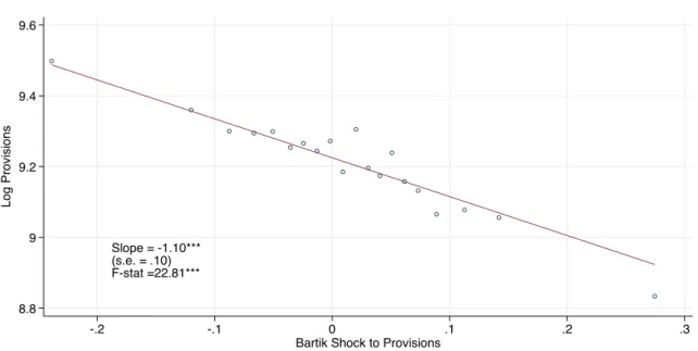
Figure3 illustrates the first-stage relationship. The first stage statistics are consistent with instrument relevance. The estimate ofψ is statistically significant (p=.003). The Kleibergen-Paap first-stage F-statistic in the baseline specification is 22.8.
The first-stage relation between legislative flow and the instrument is negative. The interpretation of our instrument is somewhat different from the standard shift-share instrument for economic shocks. Our interpretation is that when a state had initially low detail on a topic, then it is more likely to increase detail in response to national trends on that topic. This is somewhat intuitive, given that the state can then borrow legislative language at relatively low cost. Consistent with this interpretation, the
“shift” term of the instrument is positively correlated with the endogenous regressor logWst, while the “shares” term is negatively correlated (Appendix Figure A.8).
There are two approaches to identification in shift-share designs. In the first ap- proach, one assumes that the pre-period shares are conditionally exogenous (Goldsmith- Pinkham et al., 2020, Jaeger et al., 2018). In this view, the exclusion restriction hinges
Figure 3: First Stage: Impact of Shift-Share Legislative Shock on Legislative Detail
Slope = -1.10***
(s.e. = .10) F-stat =22.81***
8.8 9 9.2 9.4 9.6
Log Provisions
-.2 -.1 0 .1 .2 .3
Bartik Shock to Provisions
Notes. Binned scatterplot for the first-stage relationship (Equation3) between the shift-share instrument (horizontal axis) and the log number of provisions (vertical axis). State and year fixed effects absorbed.
on the fact that the shares (normally, sectoral composition, but in our case, topic shares) are as good as randomly assigned conditional on the fixed effects and controls (see Borusyak and Jaravel, 2017). In our case, this assumption could be formally stated as
E{Ws0k
Ws0 ·st|~αst, Xst}= 0,∀k (5) where~αstgives the vector of fixed effects. Equation (5) is a relatively strong requirement in most empirical contexts. In our case, this would mean that pre-period legislative topic shares are uncorrelated with subsequent trends in economic growth during the treatment period. This is difficult to justify, since the period legislation could be drafted in preparation for future growth trends. For example, the proportion of legislation on taxes or employment regulation in the 1950s could be correlated with growing more or less quickly in the 1960s or 1970s.
A second approach to identification, taken by Borusyak and Jaravel (2017) and Adao et al. (2019), relies on weaker assumptions. In these frameworks, the exclusion restriction follows from the conditional exogeneity of the current-period shifters, rather than from the pre-treatment shares. No assumption is needed with respect to the pre-treatment shares, and instead this approach assumes that the global shocks are
uncorrelated with the exposure-weighted average of potential outcomes. In the case of Autor et al. (2016b), for example, the identification assumption is that average unobserved determinants of economic growth across states must be unrelated to flows of Chinese imports. With panel data (as in our context), the assumption can be further relaxed. Formally, we have
E{X
r6=s
∆ logWrtk
49 ·st|~αst, Xst}= 0,∀k (6) where the terms are as above. With the inclusion of state and time fixed effects, shocks are allowed to be correlated with exposure-weighted averages of state and time-invariant unobservables, or linearly varying within state given the inclusion of state-time trends (Borusyak and Jaravel, 2017).
In line with Borusyak and Jaravel (2017) and Adao et al. (2019), we take a number of steps to assess the validity of Zst as an instrument for logWst (see Appendix C).
First, to check that the relevance of the shift-share instrument is driven by a majority of topics, we regress the increase in provisions related to a topic in a state on the increase in the total provisions related to that topic in other states and the increase in all legal provisions in that state, for every topic (including state and year fixed effects and clustering standard errors by state). We find that topic growth is statistically significant in the great majority of topics, as shown in Appendix Figure A.9. Second, we use the test for weak instruments, robust to heteroscedasticity, serial correlation, and clustering, proposed by Olea and Pflueger (2013). A rule of thumb for 2SLS is to reject the null hypothesis of a weak instrument when the effective F is greater than 23.1. In our data, the effective F statistic equals 132.794 and we reject the weak instrument null at 5 percent significance. Third, Appendix TableA.4reports the following placebo test:
we regress economic growth on future values of the legislative-growth instruments. The estimates are not statistically significant. Fourth, we run a balance test by regressing the instrument on some potential confounders. Appendix TableA.6 shows the instrument is not correlated with current or lagged values for relevant state characteristics.
Independently, we also show that we can pass the checks proposed by Goldsmith- Pinkham et al. (2020) and Jaeger et al. (2018) in the alternative framework that assumes exogeneity of pre-treatment shares. Appendix Table A.5shows that the pre-treatment topic shares are uncorrelated with pre-treatment state characteristics. Appendix Figure A.10 shows that pre-treatment topic shares are uncorrelated with subsequent growth