arXiv:1210.7948v3 [nlin.CD] 12 Feb 2013
Transport moments and Andreev billiards with tunnel barriers
Jack Kuipers and Klaus Richter
Institut f¨ur Theoretische Physik, Universit¨at Regensburg, D-93040 Regensburg, Germany
E-mail: jack.kuipers@ur.de
Abstract. Open chaotic systems are expected to possess universal transport statistics and recently there have been many advances in understanding and obtaining expressions for their transport moments. However when tunnel barriers are added, which represents the situation in more general experimental physical systems much less is known about the behaviour of the moments. By incorporating tunnel barriers in the recursive semiclassical diagrammatic approach we obtain the moment generating function of the transmission eigenvalues at leading and subleading order. For reflection quantities quantum mechanical tunneling phases play an essential role and we introduce new structures to deal with them. This allows us to obtain the moment generating function of the reflection eigenvalues and the Wigner delay times at leading order. Our semiclassical results are in complementary regimes to the leading order results derived from random matrix theory expanding the range of theoretically known moments. As a further application we derive to leading order the density of states of Andreev billiards coupled to a superconductor through tunnel barriers.
PACS numbers: 03.65.Sq, 05.45.Mt, 72.70.+m, 73.23.-b, 74.40.-n, 74.45.+c
1. Introduction
Quantum systems that are chaotic in the classical limit exhibit universal behaviour, for example for the transport through quantum dots [1, 2]. For open systems, the transport properties are encoded in the scattering matrix connecting the incoming and outgoing wavefunctions in the leads. If we imagine a chaotic cavity attached to two scattering leads carrying N1 and N2 channels respectively, with a total of N =N1+N2, then the scattering matrix separates into four blocks
S(E) =
r t′
t r′
. (1)
Of particular interest are the transmission eigenvalues and their moments Tr t†tn
given in terms of the transmission subblock of the scattering matrix. The transmission eigenvalues relate to electronic transport through the cavity, like the conductance which is proportional to their first moment [3, 4, 5] and the power of the shot noise which is related to their second.
To obtain a handle on the transport moments, one can employ the semiclassical approximation for the elements of the scattering matrix [6, 7]
Soi(E)≈ rµ
N X
γ(i→o)
Aγ(E)e~iSγ(E), (2) in terms of all the classical scattering trajectories γ that connect the corresponding channels. They contribute with their stability amplitude Aγ and a phase involving their actionSγ whileµis the escape rate of the corresponding classical system.
The first moment of the transmission eigenvalues then follows from a sum over pairs of trajectories which start in the same channel in one lead and end in the same channel in the other
Tr t†t
≈ µ N
N1
X
i=1 N2
X
o=1
X
γ(i→o) γ′(i→o)
AγA∗γ′e~i(Sγ−Sγ′). (3)
This fluctuates as the energy is varied and as we are particularly interested in the statistics of the transmission eigenvalues, we average over a range of energies. The averaging over the phase difference picks out pairs of trajectories with highly similar actions and indeed when the trajectories are identical (γ = γ′), one recovers the contribution N1N2/N [8, 9] which is the leading order term of an expansion inN−1 of the full result. The next order term was discovered to follow from trajectories that come close to themselves in an ‘encounter’ as they travel through the cavity [10]. A partner trajectory can then be found which is nearly identical, but which traverses the encounter differently. Together these pairs provide the weak localisation correction
−N1N2/N2 for systems with time reversal symmetry. Higher order corrections came from more complicated pairs of trajectories which are nearly identical in long stretches called ‘links’ while differing in small encounter regions and which could be summed to give the complete result for the first moment [11].
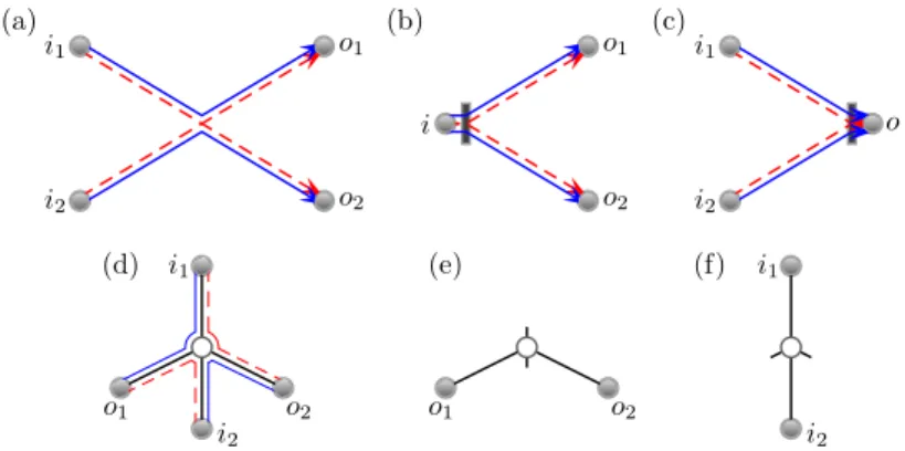
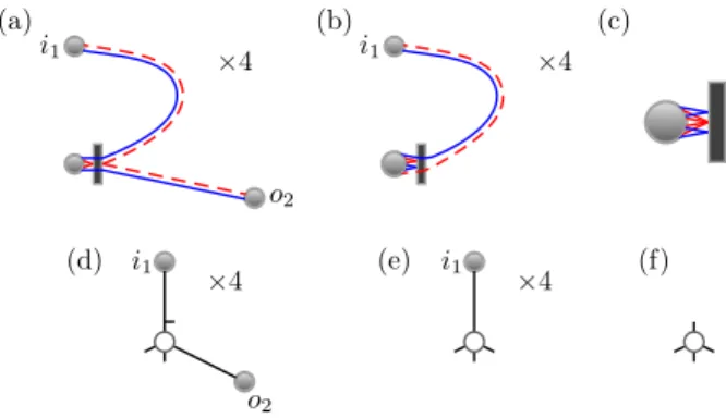
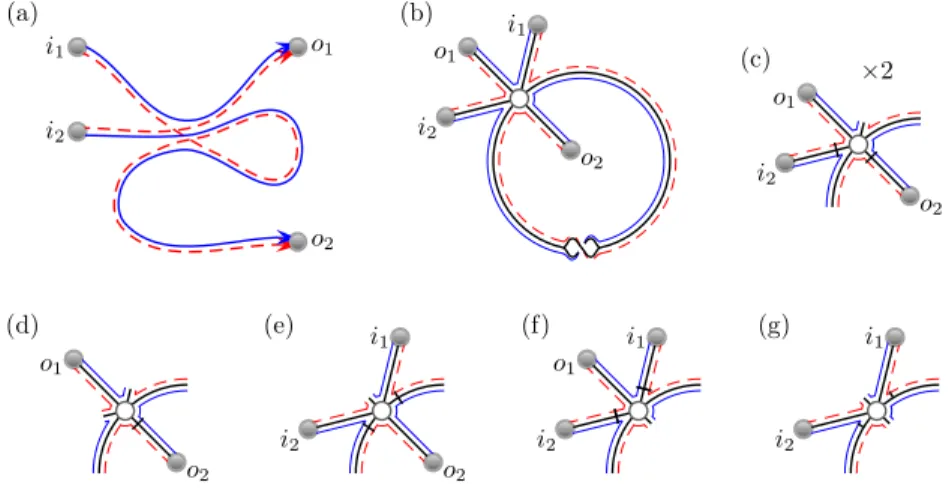
The semiclassical treatment of the first two moments and other correlations functions [11, 12, 13] led to diagrammatic rules where the contribution of any diagram could be read off from its structure. In particular, each link provides a factor of N−1, each encounter a factor of−N and each channel in the first or second lead a factor of N1 or N2. The main leading order diagram for the second moment of the transmission eigenvalues, which is pictured in figure 1(a) then provides a contribution of−N12N22/N3. From this diagram it is further possible to shift the encounter to the left until it enters the incoming lead as in figure 1(b). We note that this picture of encounters moving into leads actually derives from the semiclassical treatment of Ehrenfest time effects [14, 15, 16] where the remnant of the encounter provides an Ehrenfest time dependent factor which ensures the unitarity of the transport.
However, when the Ehrenfest time is small compared to the dwell time (the typical time that trajectories spend inside the cavity), the semiclassical contribution is as if the encounter is removed entirely and the channels in the lead coincide. The configuration in figure 1(b) then has i1 = i2 and provides a contribution of N1N22/N2. Likewise, the corresponding case of moving the encounter into the outgoing lead in figure 1(c) provides the contribution N12N2/N2. These three cases are the only possibilities at leading order, giving a total ofN ξ(1−ξ) withξ=N1N2/N2.
With the diagrammatic rules, the problem of calculating the moments reduces to that of finding all the possible diagrams, which was performed for the first two moments [11, 12, 13] through the connection to correlated periodic orbits which
(a)i1
i2
o1
o2
(b)
i
o1
o2
(c)i1
i2
o
(d)
o1
i1
i2
o2
(e)
o1 o2
(f) i1
i2
Figure 1. The trajectory quadruplet which meets at a central encounter in (a) contributes to the leading order term of the second moment. The quadruplet can be redrawn as the tree in (d) where the paths around the trees recreate the trajectories in (a). By moving the encounter to the incoming lead, with i1=i2, we obtain the possible trajectory configuration in (b), here shown with the trajectories tunneling through the barrier. Removing the paths on the left of the encounter can be represented by leaving stubs in the tree diagram as in (e).
Moving the encounter to the outgoing lead provides the structure in (c) or the tree diagram in (f).
contribute to spectral statistics of closed systems [17, 18, 19]. For higher moments instead, the leading order diagrams can be represented as trees [20]. For example, the trajectories in figure 1(a) become the tree in figure 1(d) while moving encounters into the leads corresponds to removing alternating links around the encounter node as in figures 1(e) and (f). Since trees can be generated recursively by cutting them at nodes into sets of smaller trees, all the moments of the transmission eigenvalues [20]
and the moments of the delay times [21] could be obtained at leading order in inverse channel number. This approach could also be adapted to include energy dependence and obtain the leading order behaviour of the density of states of Andreev billiards [22, 23]. Graphical recursions could then be utilised to obtain all moments of these various quantities at the next few orders in inverse channel number [24].
Exploring the combinatorial interpretation of the semiclassical diagrams, it was recently shown [25, 26, 27] that they always combine to give exactly the same results as those derived from random matrix theory (RMT) where the scattering matrix is modelled as having random elements and belonging to one of the circular ensembles [28]. In fact the semiclassical diagrams can be related to factorisations of permutations, and one combinatorial interpretation for systems without time reversal symmetry (corresponding to the unitary ensemble) was derived from the periodic orbits of closed systems [25, 27], while the other intepretation for all three classical symmetry classes reduces to primitive factorisations [26].
This equivalence between semiclassics and RMT for transport was originally put forward in the late 80’s [29, 30] and RMT was first used to calculate the conductance and its variance [31, 32] with a diagrammatic approach later providing several leading and subleading order results [33]. However, RMT also provides the probability distribution of the transmission eigenvalues [28] and their moments are given by integrals related to the Selberg integral. This connection more recently allowed the shot noise power [34] and then various fourth moments to be calculated [35] and brought a lot of interest to the evaluation of these integrals and the corresponding
transport moments. Various techniques were developed to obtain all the moments of the transmission eigenvalues [36, 37, 38, 39] and of the conductance and shot noise [37, 40, 41, 42, 43] as well as of the Wigner delay times and time delay [38, 43].
Interestingly, the different techniques tend to lead to different expressions for the moments which are not so obviously related to each other even though they must be equivalent. Similarly, the RMT and semiclassical moments must agree [25, 26]
but the resulting formulae are different enough to obscure the equivalence. However, asymptotic analyses [44] of the particular expressions for the moments obtained in [38]
have managed to recover the semiclassically calculated moment generating functions at the first few orders in inverse channel number [24].
The above discussion was for the particular case where the leads couple perfectly to the cavity, but for the more general and important case when this coupling becomes imperfect much less is known. Imperfect coupling often occurs in physical experiments in systems from microwave billiards to quantum dots and to make the theoretical treatment above of wider practical use we need to expand the framework to include the coupling. For this we add a thin potential wall or tunnel barrier at the end of the leads so that any incoming (or outgoing) particle is separated into transmitted and reflected parts, which was originally treated semiclassically in [45]. Here we show how this can be incorporated into the current graphical semiclassical framework [24].
On the RMT side the probability distribution of the transmission eigenvalues is currently unknown, with the state of the art being a cavity with one perfect and one imperfect lead [46]. The moments are likewise generally unknown apart from at leading order when the leads are identical [33]. For the delay times, the probability distribution is known [47] but the moments have yet to be evaluated. In general only the weak localisation correction to the conductance and the universal conductance fluctuations [33] along with the subleading contribution to the shot noise power [48]
have been derived diagrammatically. But these have also be obtained semiclassically by considering the diagrams explicitly [45, 49, 50] a process we now show how to perform implicitly.
Our paper is organised as follows: In section 2 we explain how tunnel barriers lead to modifications in the number of semiclassical diagrams and on the level of their individual contributions. In sections 3 and 4 we derive, to leading order, the moments of the transmission and reflection eigenvalues. Section 5 is devoted to the moments of the Wigner delay times while in section 6 we consider Andreev billiards with tunnel coupled superconducting leads as an important application. Finally in Appendix A we work out the first subleading order terms for the transmission eigenvalues.
2. Semiclassics with tunnel barriers
Introducing tunnel barriers leads to two main changes in the semiclassical diagrammatic treatment of transport. The first is that the contributions of the individual parts of the diagrams changes. The tunnel barriers can be treated probabilistically in the semiclassical limit so that trajectories have a certain probability to pass through each time they hit the barriers in the leads [45]. In general this probability pi can be different for each channel i. For an l-encounter involving l trajectory stretches of lengthtwhich are close together, if the encounter hits channel iin the leads, the joint survival probability of all the stretches is (1−pi)l. Over time,
(a)i1
i2
o1
o2
(b) i1
i2
o1
o2
(c)
i1
i2
o1
o2
×2
(d)
o1
i1
o2
(e)
o1
i2
o2
(f)
o1
i1
i2
i1
i2
o2
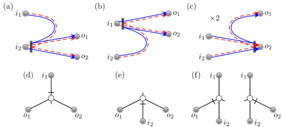
Figure 2. With tunnel barriers, trajectory stretches can additionally be reflected at the tunnel barriers. When the encounter from figure 1(a) now moves into the lead, one trajectory stretch can tunnel through while the other is reflected as in (a)–(c). In the tree representation there are four possibilities of removing one link (represented as a stub) and reflecting the other (represented by the perpendicular bar) as in diagrams (d)–(f).
the survival probability of the encounter is e−µltwith an escape rate of µl= µ
N
N
X
i=1
1−(1−pi)l, (4)
whereµis the escape rate of the same system without tunnel barriers in the lead. The diagrammatic rules for the contributions of semiclassical diagrams then become [45]:
• Each link provides the factory= PN
i=1pi
−1
• Eachl-encounter the factor−PN
i=11−(1−pi)l
• Each channel sum provides the factorPN1
i=1pji(1−pi)k or PN
i=N1+1pji(1−pi)k wherej counts the number of trajectory pairs passing through the same channel andkthe number of pairs reflected.
For example for the moments of the transmission eigenvalues, a diagonal pair starting in a channel in the incoming lead and travelling together to a channel in the outgoing lead give the leading order term of the first moment
Tr t†t
= PN1
i=1piPN i=N1+1pi
PN i=1pi
+O(1). (5)
With the same tunneling probability p in each channel, this simplifies topN ξ with ξ=N1N2/N2while the standard second moment diagram of figure 1(a) provides
− 1−(1−p)2
Np4N12N22
p4N4 =p(p−2)N ξ2. (6)
Moving the encounter fully into the leads as in figures 1(b) and (c) gives an additional p4N1N22
p2N2 +p4N12N2
p2N2 =p2N ξ. (7)
The second main change with tunnel barriers is that many additional diagrams become possible [45, 49]. Encounters can now partially enter the leads as trajectories
can be reflected back into the cavity and are no longer forced to leave the system.
Staying with the simpler example of the moments of the transmission eigenvalues, from the diagram in figure 1(a), we could move the encounter into either lead, let one trajectory pair stretch pass through the tunnel barrier and one be reflected as in figures 2(a)–(c). From the channel sum of the encounter touching the lead, we obtain a factor ofp(1−p)N1orp(1−p)N2 and an additional contribution of
2p(1−p)N1p3N1N22
p3N3 + 2p(1−p)N2p3N12N2
p3N3 = 4p(1−p)N ξ2, (8) where the factor 2 comes from the two possibilities of which trajectory to let pass through the barrier. The total result for the leading order term of the second moment of the transmission eigenvalues becomes
DTr t†t2E
=pN ξ(p+ 2ξ−3pξ) +O(1). (9) Our aim now is to systematically generate these additional possible diagrams, with their semiclassical contributions, for higher moments.
3. Moments of the transmission eigenvalues
As the moments of the transmission eigenvalues involve trajectories starting in one lead and ending in the other, the possibilities for moving encounters partially into the leads are somewhat limited. They can therefore be treated relatively easily by extending the treatment without tunnel barriers and here we mainly highlight the changes needed to incorporate them. At leading order in inverse channel number, the underlying semiclassical diagrams can be redrawn as trees [20] as going from the top lines in figure 1 and figure 2 to the bottom lines. This framework has been further developed [21, 22] and detailed in [23]. Graphical recursions can be used to go beyond leading order and we build on that formalism here using generating functions as defined in [24]. In particular we will obtain an expansion for the moment generating function
T(s) =
∞
X
n=1
snD Tr
t†tnE
=N T0+T1+. . . (10)
3.1. Tree recursions
To generate the leading order semiclassical diagrams, we start from the related tree diagrams where the encounters become vertices of even degree (≥4), the links become edges and the incoming and outgoing channels become leaves or vertices of degree 1.
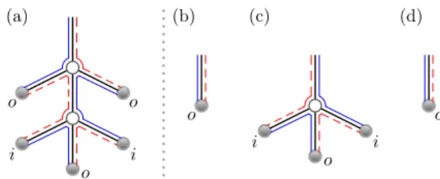
The boundary walk of the tree allows us to recover how the semiclassical trajectories are arranged. For example, the trajectories in figure 1(a) become the boundary walk of the tree in figure 1(d) and vice versa. This also means that the incoming and outgoing channels must alternate around the tree itself. To generate the trees recursively we start by not rooting them in any channel so that these intermediate trees have an odd number of leaves and therefore come in two types. One type has an excess of outgoing channels so that, if it had a root, the root would be an incoming channel and we say that this type of tree starts from an incoming direction. For example, the tree in figure 3(a) is of this type. The other type has an excess of incoming channels and starts from an outgoing direction as in figure 3(c).
We then letφand ˆφbe generating functions which count all trees (including their semiclassical contributions) starting inside the system from an incoming or outgoing
(a)
o o
i
o i
(b)
o
(c)
i
o i
(d)
o
Figure 3. For the tree recursions we start with unrooted trees which come in two types, those with an excess of outgoing channels as in (a) and (b) which belong toφand those with an excess of incoming channels as in (c) which belong to ˆφ.
By combining the top of the three trees in (b), (c) and (d) into a new encounter and adding a new link, we can create the tree in (a).
direction respectively and not rooted in any channel. The functionφincludes the trees in figures 3(a) and (b) as well as that in figure 1(d) with the channeli1 at the top removed. As the nth moment involves 2nsemiclassical trajectories with n incoming andnoutgoing channels, by including a factorrwith each channel we can track which moment each tree diagram contributes to. The variablerthen becomes the generating variable so that later the coefficient ofr2n will give thenth moment.
We can generate trees recursively since the trees start with a link which connects to an encounter of arbitrary sizel, while alternating below it arelfurther trees of the same type as the starting tree andl−1 trees of the opposite type. An example for l= 2 can be seen in figure 3(a). Similarly, bringing trees together in this way allows us to create all larger trees. Trees can be brought together only if they all start inside the system, which is why we have this restriction onφ and ˆφ.
Without tunnel barriers, forφwe could further remove all thel trees ofφtype below the encounter and move this encounter into the outgoing lead, as in figure 1(f).
We include the contribution of such diagrams (with the top channel removed again) in φ, but since the start point of φis supposed to be inside the system, the diagram in figure 1(e) is not included. Such cases will be accounted for later.
With tunnel barriers the new possibilities for the encounter are illustrated for the second moment in figure 2. In general, touching the outgoing lead involves removing anyk of thel trees and allowing the otherl−k to be reflected back into the cavity, as in figure 2(f). The case k = 0 just means that the entire encounter is reflected at the tunnel barrier and is already included in the semiclassical contribution of the encounter. The encounter could also move to the incoming lead with the first link from the starting point to the encounter reflected and k of the l−1 trees of type φˆ removed to tunnel straight into the lead instead. This possibility is illustrated in figure 2(d), while a diagram like that in figure 2(e) is not included inφ. Again the casek= 0 is already included elsewhere and we obtain the recursion relation
φ=yr
N
X
i=N1+1
pi−y
∞
X
l=2 N
X
i=1
1−(1−pi)l φlφˆl−1
+yX
l=2 N
X
i=N1+1
φˆl−1
l
X
k=1
l k
φl−k(1−pi)l−kpkirk
+yX
l=2 N1
X
i=1
φl
l−1
X
k=1
l−1 k
φˆl−1−k(1−pi)l−kpkirk. (11) The first line starts with the contribution of the smallest tree which is just a link that tunnels through into the outgoing lead as in figure 3(b). In the first line we then add all the trees whose top encounter does not move into the lead. The remaining two lines count the possibilities that the encounter moves into the outgoing or incoming lead andkof the stretches of the encounter tunnel straight through the lead (with the remaining stretches being reflected back into the cavity). Since the powers ofrcount the order of the diagram, a factorris included with each tree which is removed along with a corresponding factor ofpto record that those links have tunnelled through the barrier.
In the recursion relation we can perform the sums overk. Since the (1−p)l in the top line of (11) corresponds to thek= 0 terms of both sums, we can simplify to φ
N
X
i=1
pi=r
N
X
i=N1+1
pi−N
∞
X
l=2
φlφˆl−1+X
l=2 N
X
i=N1+1
φˆl−1(rpi+φ(1−pi))l
+X
l=2 N1
X
i=1
φl(1−pi)
rpi+ ˆφ(1−pi)l−1
, (12)
where we further divided both sides byy. Neatly, the first two terms can be rearranged into thel= 1 terms of the three sums overl, so that the recursion reduces to
N φ 1−φφˆ =
N
X
i=N1+1
rpi+φ(1−pi) 1−rpiφˆ−φφ(1ˆ −pi)+
N1
X
i=1
φ(1−pi)
1−rpiφ−φφ(1ˆ −pi). (13) For ˆφwe likewise have
Nφˆ 1−φφˆ =
N1
X
i=1
rpi+ ˆφ(1−pi) 1−rpiφ−φφ(1ˆ −pi)+
N
X
i=N1+1
φ(1ˆ −pi)
1−rpiφˆ−φφ(1ˆ −pi). (14) 3.2. Leading order moments
To obtain the leading order diagrams, we now root the top ofφin an incoming channel.
This also allows us to remove the top link and tunnel straight into an encounter in the incoming lead, so we can now add diagrams like figure 1(e) and figure 2(e). Of the remainingl−1 alternating ˆφtrees emanating from the encounter, anykcan also move straight into the lead. The generating functionT0, which counts all the leading order diagrams with their contributions and divided byN, is then given by
N T0=
N1
X
i=1
rpiφ+
N1
X
i=1
pir
∞
X
l=2
φl
l−1
X
k=0
l−1 k
φˆl−1−k(1−pi)l−1−kpkirk, (15)
Performing the sums gives N T0=
N1
X
i=1
rpiφ
1−rpiφ−φφ(1ˆ −pi). (16)
3.3. Fixed tunneling probabilities in each lead
With the formulae in (13), (14) and (16) we have a formal generating function for the leading order terms of all moments and we can expandφ, ˆφand thenT0in powers ofr.
However, with the sums over the different tunneling probabilities in each channel, it is difficult to manipulate the expressions further. To proceed we can make the simplifying assumption that the channels in each lead have the same tunneling probability of p1
for the incoming lead andp2 for the outgoing lead. Equations (13) and (14) lead to quartic equations forφand ˆφwhich in turn lead to the following quartic equation for T0:
(s−1) s2p21p22+ 2sp1p2(2−p1−p2) + (p1−p2)2 T04 +2s(s−1)p1p2(sp1p2+ 2−p1−p2)T03
+s
s(s−1)p21p22+p21(p2−1)ζ1+p22(p1−1)ζ2
+ξ 2sp1p2(2−p1−p2) +s(2s−1)p21p22+ (p1−p2)2 T02 +s2p21p22ξ(2s−1)T0+s3p21p22ξ2= 0, (17) whereζ1=N1/N,ζ2 =N2/N and r2=sis the generating variable for the moments since thenth moment involves trees with 2nleaves. ExpandingT0 in powers of swe need to choose the correct value for the first moment, which isp1p2ξ/(p1ζ1+p2ζ2) from (5).
3.4. One perfect lead
Equation (17) allows us for example to consider the situation where only one of the leads has a tunnel barrier by setting p1 or p2 to 1, as in the recently considered situation where the probability distribution of the reflection eigenvalues was obtained from RMT for systems without time reversal symmetry [46] although with different tunneling probabilities in the channels in the remaining lead. With equal probabilities instead andp2= 1, we actually obtain a cubic equation semiclassically
(s−1) (1 +p1(s−1))T03+s(s−1)p1(1 +ζ2)T02
+s(ξ+p1ξ(s−1) +ζ2(sp1−1))T0+s2p1ξζ2= 0, (18) which can also be obtained from (17) through usingξ =ζ1ζ2 and ζ1 = 1−ζ2. The generating function in (18) should then match the leading order moments found by integrating the corresponding transmission probability distribution to that in [46].
3.5. Equal tunneling probabilities
To proceed further we instead set all of the tunneling probabilities equal top=p1= p2. The quartic equation forφnow has the expansion
φ=ζ2r+ξ(p+ζ2(1−2p))r3+
+ξ p2+pζ2(1−2p) +pξ(3−5p) + 2ζ2ξ[1−5p(1−p)]
r5. . . (19) while for ˆφwe swapζ2 andζ1. The second term in (19) corresponds to the sum of the diagrams in figures 1(d) and (f) and figures 2(d) and (f). The quartic forT0reduces to
(s−1) sp2+ 4(1−p)
T04+ 2(s−1) sp2+ 2(1−p) T03 +
s(s−1)p2+p−1 +sξ 4(1−p) + (2s−1)p2 T02
+s(2s−1)p2ξT0+s2p2ξ2= 0, (20)
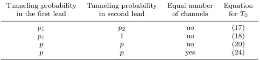
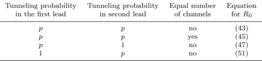
Table 1.Leading order generating functions for the moments of the transmission eigenvalues for different restrictions on the tunneling probability and number of channels in each lead.
Tunneling probability Tunneling probability Equal number Equation in the first lead in second lead of channels forT0
p1 p2 no (17)
p1 1 no (18)
p p no (20)
p p yes (24)
and again for the expansion in powers ofswe need to pick the correct value ofpξ for the first moment (since we dividedT0byN). The first few terms in the expansion are
T0=pξs+pξ(p+ 2ξ−3pξ)s2
+pξ p2+ 2p(3−4p)ξ+ (6−21p+ 17p2)ξ2
s3+. . . (21) with the second term corresponding to the second moment calculated explicitly in section 2.
3.6. Equal leads
As a further simplification, we can also have an equal number of channels in each lead so thatζ1=ζ2= 1/2. Due to the symmetry we haveφ= ˆφ, so (12) reduces to
2φ
1−φ2 = rp+ 2φ(1−p)
1−rpφ−φ2(1−p), rφ2−2φ+r= 0, (22) whereφis actually given by the same quadratic as when there are no tunnel barriers in the leads. The moment generating function then satisfies the quadratic equation
4(s−1) sp2+ 4(1−p)
T02+ 4(s−1)sp2T0+s2p2= 0, (23) which is also a factor of (20) whenζ1=ζ2= 1/2 orξ= 1/4. The moment generating function can then be given explicitly as
T0= sp p(1−s) + (p−2)√ 1−s
2(s−1) (sp2+ 4(1−p)) , (24)
where we chose the solution of (23) which matches the first momentp/4.
3.7. Summary of different results
We summarize the restrictions for the results in the different cases above and detail which generating function is appropriate for which situation in Table 1.
3.8. Comparison with RMT
The RMT result for the leading order probability distribution of the transmission eigenvalues was calculated in [33]. However, a final result could be obtained if they assumed the two leads were identical. The channels could have different individual tunneling probabilities though, as long as the probabilities are matched in the other lead. The result [33] was
P(Z) =
N1
X
i=1
pi(2−pi) π(p2i −4piZ+ 4Z)p
Z(1−Z). (25)
Semiclassically instead it is simple to have different sized leads, but with a constant tunneling probability in each. To compare the different results we can look at the common results for the simplest case of identical leads with a single tunneling probability. From the moment generating function in (24), including the 0th moment as 1, we can perform the Hilbert transformation to get the probability density 1 +T0=
Z 1
0
P(Z) N
1
1−sZdZ, P(Z)
N = p(2−p)
2π(p2−4pZ+ 4Z)p
Z(1−Z), (26) which is exactly (25) with identical tunneling probabilities. That the distribution in (25) for identical leads is a sum over the channels means that the moment generating function would likewise be a sum over terms like in (24) again with different pi. Semiclassically, with identical leads we have φ = ˆφ through symmetry, but this result still cannot easily be seen from (13) and (16). Instead we have access to the complementary regime of different leads with equal tunneling probabilities.
We can proceed to higher orders in the inverse number of channels (see [10]) by similarly modifying the approach [24] without tunnel barriers. For example, we present the calculation ofT1in Appendix A. However, the more interesting case occurs when we consider reflection quantities.
4. Moments of the reflection eigenvalues
When we consider the moments of the reflection eigenvalues, or their generating function
R(s) =
∞
X
n=1
snD Tr
r†rnE
=N R0+R1+. . . (27) we now have a semiclassical approximation where the trajectories all start and end in the same lead. With tunnel barriers, this allows even more diagrammatic possibilities when moving encounters into the lead, and we may also have trajectories that never enter the system and are reflected instead directly at the tunnel barrier [45, 49]. For example for the second moment, along with the diagrams in figures 1 and 2, the diagrams in figure 4 are also now possible.
Along with the additional possibilities, the tunneling phases now become particularly important [45]. Looking in detail at the tunnel barrier drawn in figure 4(a), where the incoming channeli2is identical to the outgoing channelo1, both solid trajectories tunnel through while both dashed, complex conjugated, trajectories are reflected, one on each side of the barrier. If ρis the reflection amplitude of the barrier andτthe transmission amplitude then the four trajectories of the encounter at the barrier give the factor (τ ρ∗)2which in the semiclassical limit is equal to−p(1−p) with an additional minus sign arising from the quantum mechanical tunneling [45].
With equal tunneling probabilities in every channel, the diagrams in figures 4(a) or (d) then give a total semiclassical contribution of
−4p(1−p)N1
p2N12
p2N2 =−4p(1−p)N ζ13. (28) In figures 4(b) or (e), the tunneling and reflecting trajectories at the tunnel barrier pair a trajectory stretch with a complex conjugated one giving the standard factor ofp(1−p) while in figures 4(c) or (f) none of the trajectories ever enter the system.
Combined they give
4p(1−p)N ζ12+ (1−p)2N ζ1, (29)
(a)i1
o2
×4
(b)i1
×4 (c)
(d) i1 ×4
o2
(e) i1 ×4 (f)
Figure 4. For reflection quantities incoming and outgoing channels can coincide so that with tunnel barriers new possibilities arise for encounter stretches to tunnel into the lead. Allowing the stretch to channel o2 from figure 2(a) to also tunnel into the lead so that channels o1 = i2 give the possible diagram in (a). In the graphical representation in (d) this corresponds to removing adjacent links around the encounter node, which can be performed in 4 ways. We can remove an additional link as in (b) and (e), ifo2=o1=i2where now a pair of trajectories are directly reflected at the tunnel barrier, and finally have the situation in (c) and (f) where none of the trajectories ever enter the system.
while the diagrams in figures 1 and 2 provide the contribution
p(p−2)N ζ14+ 2p2N ζ13+ 4p(1−p)N ζ14, (30) since now all the channels are in the first lead. We can then, using ζ1(1−ζ1) =ξ, write the leading order term of the second moment of the reflection eigenvalues as
DTr r†r2E
=N ζ1+pN ξ(p−2 + 2ξ−3pξ) +O(1). (31) Through the unitarity condition, we have
r†r+t†t=IN1, Tr r†r2
=N1−2 Tr t†t
+ Tr t†t2
, (32) which is satisfied by the leading order second moments in (9) and (31) since the leading order first moment of the transmission eigenvalues from (5) ispN ξ.
4.1. Auxiliary trees
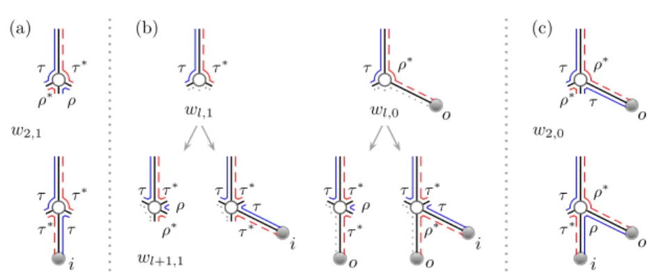
For the moments of the reflection eigenvalues, we first let f and ˆf be generating functions which count all trees including their semiclassical contributions which start inside the system from an incoming or outgoing direction respectively (without being rooted in a channel). Due to the symmetry, we actually havef = ˆf but we will treat them separately for now. The f trees, which now include diagrams like figures 4(a) and (b) with the channel i1 removed, initially start from a link connecting to an l- encounter which is followed bylsubtrees of typef andl−1 trees of type ˆf. In general, and as illustrated in figure 4, we can now allow any of the links around an encounter node to tunnel straight into the lead and be removed in the graphical representation.
Counting the possibilities recursively would be straightforward, but for the quantum mechanical tunneling phases which actually depend on how many adjacent links are removed together. To keep track of these phases we introduce auxiliary generating functionswl,αand ˆwl,α which count the contributions below the encounter (and not the top link off) and where the encounter is in a particular channel in the
(a)
τ ρ∗ ρ
τ∗
w2,1
i τ τ∗ τ
τ∗
wl,1 τ τ∗ (b)
wl+1,1
τ ρ∗
ρ τ∗
i τ
τ∗ τ τ∗
wl,0 o τ ρ∗
o τ
τ∗ ρ τ∗
i o τ
ρ∗ τ τ∗
(c)
o τ
ρ∗ τ ρ∗
w2,0
i o τ
τ∗ ρ ρ∗
Figure 5. For the auxiliary generating functions w where the first link after the encounter node tunnels directly into the lead, we need to track exactly which trajectories tunnel through or are reflected at the barrier. Forwl,1 the last link tunnels so that, depending on whether the middle link tunnels or is reflected, there are two possible configurations inw2,1 as shown in (a). For wl,0 the last link is reflected so that again there are two configurations inw2,0 shown in (c).
Starting from all the configurations in wl,1 andwl,0 we can add an additional two links on the right of the encounter. If the last tunnels into the lead, the two possibilities for the other generate the configurations inwl+1,1as depicted in (b) while if the last link is reflected we obtainwl+1,0 and the recursions in (35).
lead with tunneling probabilityp. The subscriptα= 1 represents that the last of the subtrees tunnels straight into the lead and is removed from the diagram and α= 0 represents that it is reflected. Inw we ensure that the first subtree tunnels into the lead while in ˆwwe ensure it is reflected. The smallest encounter isl= 2 for which the central tree can either tunnel or be reflected so, as in figures 5(a) and (c), we have w2,1=τ ρ∗ρτ∗r3+ (τ τ∗)2r2f ,ˆ w2,0= (τ ρ∗)2r2f+τ τ∗ρρ∗rff ,ˆ (33) and
ˆ
w2,1= (ρτ∗)2r2f+ρρ∗τ τ∗rff ,ˆ wˆ2,0=ρτ∗τ ρ∗rf2+ (ρρ∗)2f2f ,ˆ (34) where for simplicity we have included an encounter entirely reflected at the lead in ˆw2,0
which needs to be remembered later. With the symmetry we also havew∗l,0= ˆwl,1and we can simplify by settingτ τ∗=p,ρρ∗= (1−p) and (τ ρ∗)2= (ρτ∗)2=−p(1−p).
Since we know the behaviour of the subtrees at the edges, we can recursively generatewl+1,afromwl,aby adding two more subtrees on the right and allowing both possibilities for the first. Tracking the trajectories as in figures 5(b) we obtain
wl+1,1=wl,1
hρρ∗r2+τ τ∗rfˆi +wl,0
τ∗ρτ∗
ρ∗ r2+τ τ∗rfˆ
, wl+1,0=wl,0
hτ τ∗rf+ρρ∗ffˆi +wl,1
ρ∗τ ρ∗
τ∗ rf+ρρ∗ffˆ
, (35) where the terms with fractions involve replacing a reflecting trajectory by a transmitting one or vice versa, and have the valuesτ∗ρτ∗/ρ∗=−pandρ∗τ ρ∗/τ∗ = (p−1). Because this recursion does not depend on whether the first subtree tunnels or is reflected, we have the same equations for ˆw. We wish to sum over encounters of all sizes, so if we set wα =P∞
l=2wl,α, and likewise for ˆw we obtain the following coupled equations
w1−p(1−p)r3−p2r2fˆ=w1
h(1−p)r2+prfˆi
+w0prh fˆ−ri
,
w0−p(1−p)rf( ˆf−r) =w0
hprf+ (1−p)ffˆi
+w1(1−p)fh fˆ−ri
. (36)
We obtain a similar equation for ˆwand the solutions, withf = ˆf, are w1= pr2[r(1−p−f2)−pf]
1−(1−p)r2−2prf−(1−p−r2)f2, w0= ˆw1= prf(p−1)(r−f)
1−(1−p)r2−2prf−(1−p−r2)f2, ˆ
w0= f2(1−p)[f(1−p−r2) +pr]
1−(1−p)r2−2prf−(1−p−r2)f2.
(37) 4.2. Tree recursions
To obtain the generating functionf we simply add a link to these contributions and sum over all channels in the lead
f y =r
N1
X
i=1
pi−
∞
X
l=2 N
X
i=1
f2l−1+
∞
X
l=2 N
X
i=N1+1
(1−pi)lf2l−1+
N1
X
i=1
(w1+ 2w0+ ˆw0), (38) where the sum over the (1−pi)l terms in the first lead are already included in ˆw0. With equal tunneling probabilities in all the channels, this is
f
1−f2 =f(1−p)[1−ζ1f2(1−p)]
1−f2(1−p) +ζ1(rp+w1+ 2w0+ ˆw0), (39) which leads to a quartic forf whose expansion is
f =ζ1r+ξ(1−p−ζ1(1−2p))r3+ (40) +ξ (1−p)2−ζ1(1−p)(1−2p)−ξ(1−p)(2−5p) + 2ζ1ξ[1−5p(1−p)]
r5. . . The second term now corresponds to the sum of the diagrams in figures 1(d) and (f) and figures 2(d) and (f) along with two new possibilities like the diagram in figure 4(d) and one diagram like figure 4(e).
4.3. Leading order moments
To move from the generating function f to the leading order moment generating function for the reflection eigenvaluesR0 we need to add a channel to the top of the diagrams inf and also allow the top link inf to tunnel straight into the lead. Since we know whether both the outside subtrees of w and ˆw tunnel or are reflected we can simply replace their top lead by a tunneling one and replace the corresponding transmitting and reflecting eigenvalues of the trajectories
N R0=
N1
X
i=1
rpif+
N1
X
i=1
r ρρ∗
τ τ∗w1+ρτ∗
τ ρ∗w0+ρτ∗
τ ρ∗wˆ1+τ τ∗ ρρ∗wˆ0
+
N1
X
i=1
r2(1−pi), (41) where the last term is the contribution to the first moment from a trajectory pair that never enters the system. We haveρτ∗/(τ ρ∗) =−1 so that in total we obtain
N R0=
N1
X
i=1
rζ1[r(1−pi−f2) +pif]
1−(1−pi)r2−2pirf−(1−pi−r2)f2. (42)
With equal tunneling probabilities, we again obtain a quartic forR0 which can be simplified to
4(s−1)(1−p) +sp2
R˜40+ ˜R30+sξR˜20
+sp2R˜03 +
(s+p−1)(1−s+sp) +sp2ξR˜02+s(1 +s)p2ξR˜0+s2p2ξ2= 0, (43) where ˜R0= (1−s)R0−ζ1sremoves theζdependence. The expansion provides R0=ζ1(s+s2+s3)−pξs+pξ(p−2 + 2ξ−3pξ)s2
−pξ p2−3p+ 3−(6−15p+ 8p2)ξ+ (6−21p+ 17p2)ξ2
s3+. . . (44) The coefficient ofs2 is the same as (31) and unitarity can be checked against (21).
With equal leadsζ1= 1/2, we end up with the same quadratic rf2−2f+r= 0 that we had for the transmission, while the moment generating function is
R0=s(2−p) (2−p)(1−s) +p√ 1−s
2(s−1) (4(s−1)(1−p) +sp2) . (45) Transforming to the probability distribution of the reflection eigenvalues, we have the same density as in (26) but withZ replaced by 1−Z which is the same mapping as between the transmission and reflection eigenvalues.
4.4. One perfect lead
Since the start and end channels are all in the same lead, is it straightforward to make the other lead transparent. Keepingpi=pin the first lead and settingpi = 1 in the second means that we remove the sum over the channels in the second lead in (38) and set 1/y=N(pζ1+ζ2). This changes (39) to
f
1−f2 =ζ1f(1−p) +ζ1(rp+w1+ 2w0+ ˆw0), (46) while (42) remains the same. This leads to a cubic forf and R0, where again using R˜0= (1−s)R0−ζ1sleads to the simpler form
(s+p−1) ˜R30+sp(1 +ζ2) ˜R20
+s[(1−s+sp)ζ2+ (s+p−1)ξ] ˜R0+s2pζ2ξ= 0. (47) Of course we could instead allow the first lead to be transparent and setpi = 1 there andpi=pin the second lead. In this case the encounters can no longer partially enter the lead so the number of possible diagrams is drastically reduced to just those where the encounter enters the lead fully. We actually then have almost exactly the same recursions as when there are no tunnel barriers in either lead, but just with the minor corrections to the survival probabilities of the encounters and links. As in [24]
we obtain
f
N y =rζ1−
∞
X
l=2
f2l−1+rζ1
∞
X
l=2
rl−1fl−1+ζ2
∞
X
l=2
(1−p)lf2l−1, (48) where the last term is due to the change in the survival probability of the encounters while the links provide 1/(N y) =ζ1+pζ2. Simplifying we get
f
1−f2 = rζ1
1−rf +(1−ζ1)(1−p)f
1−(1−p)f2 , (49)
Table 2. Leading order generating functions for the moments of the reflection eigenvalues for different restrictions on the tunneling probability and number of channels in each lead.
Tunneling probability Tunneling probability Equal number Equation in the first lead in second lead of channels forR0
p p no (43)
p p yes (45)
p 1 no (47)
1 p no (51)
where the last term is the correction due to the tunnel barrier. The moment generating function is still given by
R0= rζ1f
1−rf, (50)
which leads directly to the cubic
(s−1)(s+p−1)R30+s[ζ1(3s+ 2p−3)−p]R20
+sζ1[ζ1(3s+p−1)−p]R0+s2ζ13= 0. (51) Shifting the generating function as before, ˜R0= (1−s)R0−ζ1s, we then obtain exactly (47) but withζ2 replaced byζ1, which leaves ξunchanged. Swapping ζ1 and ζ2 just means we are considering the moments of the reflection eigenvalues of the second lead
R′(s) =
∞
X
n=1
snTrh r′†r′in
=N R′0+R′1+. . . (52) while the unitarity conditionr′r′†+tt†=IN2 ensures that
R(s)− N1s
1−s =R′(s)− N2s
1−s, (53)
so this much simpler treatment provides the same generating function (47) as the full auxiliary tree combinatorics when one lead is transparent. This leading order generating function should also arise as the first term of an asymptotic expansion of the recently derived RMT probability distribution [46] when the remaining tunneling probabilities are set equal.
4.5. Summary of different results
A summary of the different restrictions considered above and the resulting moment generating functions is given in Table 2.
5. Moments of the Wigner delay times
The tree recursions for the moments of the reflection eigenvalues can easily be modified to obtain energy dependent generating functions like
C(ǫ, n) = 1 N Tr
S†
E−ǫµ~ 2
+S
E+ǫµ~ 2
n
, (54)
which are related to other physical observables like the density of states of Andreev billiards and the moments of the Wigner delay times. The generating functionG(s) =
P∞
n=1snC(ǫ, n) can be obtained by simply considering the reflection eigenvalues with a single lead ζ1= 1 and including the energy difference. This changes the encounter and link contributions to
−N(1−(1−p)l−la), y−1=N(p−a), (55) respectively witha= iǫ. The tree generating function becomes
f
1−f2 =f(1−p) + af
[1−f2]2 +rp+w1+ 2w0+ ˆw0, (56) whilewand ˆwremain unchanged. The terms can be combined and simplified to
f(1−f2−a)
[1−f2]2 = pr+ (1−p−r2)f
1−(1−p)r2−2prf−(1−p−r2)f2. (57) The leading order generating functionG0 is still given by (42) withζ1= 1 so that we obtain a quartic equation forf andG0.
We show how to use the energy dependence to obtain the leading order contribution to the density of states of Andreev billiards next in section 6 and concentrate here on the moments of the Wigner delay times. The delay times are the eigenvalues of the Wigner-Smith matrix [51, 52]
Q= ~
iS†(E)dS(E)
dE , (58)
and are a measure of the time spent inside the scattering cavity. Their moments can be obtained [21, 24, 53] through the correlation functions
D(ǫ, n) = 1 N Tr
S†
E−ǫµ~ 2
S
E+ǫµ~ 2
−I n
, (59)
by differentiating
Tr [Q]n= 1 (iµ)nn!
dn
dǫnD(ǫ, n)
ǫ=0. (60) If we denote the moment generating function by
M(s) =
∞
X
n=1
µnsnhTr [Q]ni, (61)
then we can obtain an expansion for the leading order lower moments by expanding (59) binomially and simply substituting the correlation functionsC(ǫ, n)
M0(s) =s+2 ps2+ 6
p2s3+2(p+ 10)
p3 s4+10(2p+ 7)
p4 s5+. . . (62)
5.1. Tree recursions
However to obtain the full moment generating function we need to account for the identity matrix in the brackets in (59) that creates the difference from (54). As was the case without tunnel barriers [21, 24], this matrix can be thought of as coming from diagonal trajectory pairs which just travel directly from the incoming to outgoing channels with no energy difference. With tunnel barriers, such diagonal pairs can be formed whenever an encounter goes into the lead and an ˆf subtree remains, as long as the other trajectories either side end in the lead so that we have stubs either side.
The subtree contribution already includes a diagonal pair and to subtract the identity matrix we just subtract the contribution of a diagonal pair with no energy difference
(a= 0). For every ˆf subtree surrounded by two stubs we then replace its contribution by ˆf −r/p. This breaks the symmetry between f and ˆf and we look at their two generating functions separately.
The auxiliary tree recursions forf, make it easy to see when a ˆf subtree is added with a stub either side. Modifying the recursions appropriately we find
w1−p2r2( ˆf −r) =pr( ˆf −r)(w1+w0), w0−p(1−p)rf( ˆf−r) =w0
hprfˆ+ (1−p)ffˆi
+w1(1−p)f( ˆf−r), (63) and similar equations for ˆw. This leads to the equation forf
f(1−ffˆ−a)
[1−ffˆ]2 = pr+ (1−p−pr2)f
1 +pr2−pr(f + ˆf)−(1−p−pr2)ffˆ−pr3f. (64) For ˆf however, because we add two new subtrees on the right in the auxiliary tree recursions, it is not so straightforward to see when a ˆf subtree is surrounded by two stubs. Instead we can simply add either a ˆf subtree or a stub to either side of the auxiliary trees forf. Doing so we find
fˆ(1−ffˆ−a)
[1−ffˆ]2 = pr(1 +r2) + (1−p−pr2) ˆf
1 +pr2−pr(f + ˆf)−(1−p−pr2)ffˆ−pr3f, (65) which, by multiplying (64) by ˆfand (65) byf, leads to the simple relation ˆf = (1+r2)f and a quartic equation forf or ˆf.
5.2. Leading order moments To obtain the generating function
L(s) =
∞
X
n=1
snD(ǫ, n) (66)
we then either rootfin an incoming channel or tunnel straight into the auxiliary trees to obtain
L0
r =pf−w1−w0−wˆ1+ p
(1−p)wˆ0−pr, (67)
where we included the correction−rw1/pfrom the diagonal pair above the auxiliary w1trees which have stubs on either side. The last term stems from a pair of trajectories that never enter the system. Here thewterms correspond to the auxiliary trees from the recursions forf as in (63) so that finally we obtain
L0= pr(f−r−2r2f+rffˆ)
1 +pr2−pr(f+ ˆf)−(1−p−pr2)ffˆ−pr3f, (68) and the quartic
p2(1 +s)L40+ 2aps(1 +s)(2−p)L30 +s
(ap−a+p)(a−p) +ap(ap−2p+ 4)s+a2p2s2 L20
+a2p2s2(1 + 2s)L0+a2p2s3= 0. (69) For thenth moment of the delay times we then differentiatentimes (and divide by n!) which can be achieved by simply transforming s → s/a. Setting the energy differenceato 0 then provides the generating function
pM03+ (4s−2ps−p)M02+ps2M0+ps2= 0. (70)
![arXiv:1210.7948v1 [nlin.CD] 30 Oct 2012](data:image/gif;base64,R0lGODlhAQABAIAAAP///wAAACH5BAEAAAAALAAAAAABAAEAAAICRAEAOw==)