–
Documentation of the database
Lukas Asp¨ ock, Michael Vorl¨ ander
RWTH Aachen, Institute of Technical Acoustics, Kopernikusstr. 5, D-52074 Aachen, Germany
{las; mvo}@akustik.rwth-aachen.de
Fabian Brinkmann, David Ackermann, Stefan Weinzierl TU Berlin, Audio Communication Group,
Einsteinufer 17c, D-10587 Berlin, Germany
{fabian.brinkmann; david.ackermann; stefan.weinzierl}@tu-berlin.de
September 1, 2020
Contents
1 Introduction 1
2 Content of the database 1
2.1 Scene descriptions . . . 2
2.1.1 Geometry . . . 2
2.1.2 Pictures . . . 2
2.1.3 Impulse responses . . . 2
2.2 Source and receiver descriptions. . . 3
2.3 Surface descriptions . . . 4
2.4 Additional data . . . 5
3 Acquisition of the database 5 3.1 Geometry . . . 5
3.2 Surface descriptions . . . 7
3.2.1 Absorption coefficients . . . 7
3.2.2 Scattering coefficients . . . 9
3.3 Source and receiver descriptions. . . 9
3.3.1 Source Directivities. . . 9
3.3.2 Receiver Directivies . . . 10
3.4 Impulse Responses . . . 11
3.4.1 Omnidirectional Receivers . . . . 11
3.4.2 Binaural Receiver . . . 11
BRAS: Reference scenes 15 RS1: Simple reflection (infinite plate) . . . . 16
RS2: Simple reflection and diffraction (finite plate) . . . 17
RS3: Multiple reflection (finite plate). . . 18
RS4: Simple reflection (reflector array) . . . . 19
RS5: Simple diffraction (infinite edge) . . . . 20
RS6: Diffraction (finite body) . . . 21
RS7: Multiple diffraction (seat dip effect) . . 22
Appendix: Complex rooms 23 CR1: Coupled rooms (laboratory & reverber- ation chamber) . . . 24
CR2: Small room (seminar room). . . 25
CR3: Medium room (chamber music hall) . . 26
CR4: Large room (auditorium) . . . 27
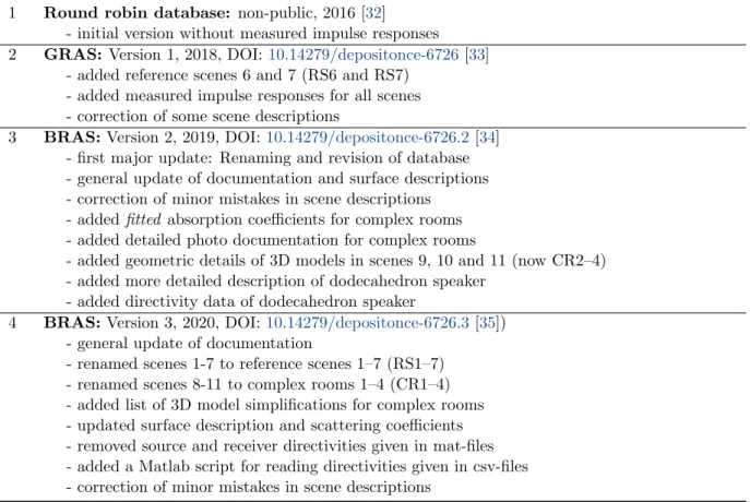
Version History 28
1 Introduction
The Benchmark for Room Acoustical Simulation (BRAS) contains reference scenes (RS) that are in- tended for the evaluation of acoustic simulation soft- ware by a comparison of measured and simulated im- pulse responses. The informal appendix of the BRAS contains complex rooms (CR) of different shape and size. Due to an increased measurement uncertainty the CRs cannot serve as a direct reference but may be used to compare the results from different simulations based on indentical input data. This document describes the data structure and format along with the acquisition of the data, while the concept of the database is detailed in an accompanying publication.
This documentation is structured as follows. The content and structure of the database is described in Section2. This is the most important sections for users of the database. The acquisition of the database is detailed in Section 3. Although this information is not required to use the database, it will help to in- terpret differences between simulations and measure- ments. Appendix A and B introduce the scenes one by one including useful information for running simu- lations such as the temperature and humidity at the time the measurements were conducted. Appendix C summarizes the history of the database.
2 Content of the database
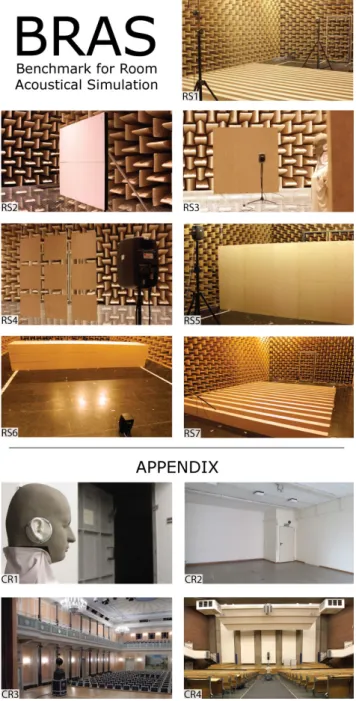
An overview of the BRAS scenes is given in Fig. 1.
The data are organized in different folders that hold scene specific and unspecific content:
1 Scene descriptions: Contains the descriptions of the scenes by means of 3D SketchUp models, pictures, and in some cases a list of details that are omitted in the models.
2 Source and receiver descriptions: Contains the directivities of the sources and receiver that were used for the creation of the BRAS along with some additional information.
3 Surface descriptions: Contains third octave absorption and scattering values and pictures of all surfaces specified in the 3D models.
4 Additional data: Contains data for comparing simulations and measurements.
The database is separated into multiple zip-files. Un- der UNIX based operating systems, the files can be extracted into their original folder structure using the terminal command unzip \*.zip after changing the working directory to the folder that contains the zip files. In Windows the default unzipping tool can be used. In this case, confirm that the files are merged into already existing folders.
Figure 1: Scenes of the BRAS and its appendix. Num- bers refer to Table2.
2.1 Scene descriptions
The folder 1 Scene descriptions contains one sub- folder for each scene including the scene specific data.
2.1.1 Geometry
The subfolder Geometry contains 3D models of the scene saved as SketchUp files and screenshots to gain a quick overview. All files are named according to the scheme sceneNo IRtype, e.g. CR3 RIRdefines the geometry of the medium room for simulating single- channel room impulse responses, whereasCR3 BRIRde- fines the same room with source and receiver positions for simulating two-channel binaural room impulse re-
sponses. In some cases, a scene is divided into sub- scenes, which is noted by sceneNo IRtype subScene, e.g. RS1 RIR Diffusor.
Each SketchUp file contains a 3D model of the scene and the names, positions, and orientations of the sources and receivers. Textures are assigned to the sur- faces of the 3D models to specify their material, e.g., mat RockFonSonarG (cf. Section 2.3). To view the texture of a surface in SketchUp, use theSample Point option of thePaint Bucket Tool. If the object belongs to a group or a component, double click it in the edit mode before using thePaint Bucket Tool.
Source and receiver positions are marked with 3D icons and text labels that specify the position of the reference points (cf. Section 3.3 and Table 4). The labes are namedLSno typefor the sources (loudspeak- ers), and MPno type for the receivers (microphones).
For example LS1 Genelec8020c gives the position of the scene’s first source, in this case a Genelec 8020c speaker. Directivities according to the labels are lo- cated in the corresponding folders (cf. Section 2.2).
The correct position and orientation is always given in the label – the positions of the 3D icons might show slight deviations.
Positions are specified with respect to the global co- ordinate system of the scene whereϕ[◦] gives the orien- tation in the horizontal plane (x/y plane,ϕ= 0 point- ing in positive x-direction,ϕ= 90 pointing in positive y-direction), and ϑ [◦] specifies the elevation (ϑ = 90 pointing in positive z-direction, ϑ = −90 pointing in negative z-direction).
Not all details of the complex rooms could be cap- tured and a list of model simplifications is provided in these cases. Despite this, the models exhibit a high de- gree of detail and might have to be further simplified for use with geometrical acoustics algorithms. In addi- tion, a model showing the setup of the QSC-K8 speaker is contained in the database for scenesCR2– CR4.
2.1.2 Pictures
The subfolderPicturescontains panorama and detail photographs of the scenes including a scale.
2.1.3 Impulse responses
The measured room impulse responses (RIRs) and bin- aural room impulse responses (BRIRs) are contained in the subfolders RIRs andBRIRs. They are provided as SOFA files [1] and wav-files with a sampling rate of 44.1 kHz. The SOFA files contain all IRs of one scene and hold additional meta data, while one wav file is given for each IR. In case of the binaural impulse responses, the first wav-file channel holds the left ear data.
The files are named sceneNo type addInfo.type, e.g.,RS1 RIRs Rigid.sofaholds all IRs for theRigid sub-scene of scene 1, whereas the IR for a specific loudspeaker-microphone combination of the same scene
is given in RS1 RIR Rigid LS1 MP3.wav. For scenes CR1 - CR4, RIRs were measured for 4 different ori- entations of the Genelec 8020c. This is denoted by LSorientationas detailed inAppendix B.
Level Calibration
This section describes the level calibration of the mea- surements. The simulations should be calibrated ac- cordingly.
RIRs: To establish an absolute sound pressure level, the input chain was calibrated with a microphone cali- brator. The output chain was calibrated to a free field sound pressure of 80 dB at 1 kHz and a distance of 2 m in front of the loudspeaker, i.e., Φ=Θ= 0◦ (Fig- ure 3a). Consequently, the RIR unit is Pascal.
BRIRs: Because the BRIRs are intended for auraliza- tion and were thus normalized by a single, frequency independent gain factor per scene as detailed in Sec- tion3.4.2. Consequently, the BRIRs are unit-less.
SOFA files
The SOFA files can be read with various APIs and store the IRs in the field Data.IR. The dimensions of Data.IRare listed inTable 1and differ among scenes and IR types (RIR, BRIR). The additional meta data entries EmitterID and ReceiverID give the order of the IR and specify the source and receiver according to the labels of the 3D models (cf. Section. 2.1.1).
E.g., the IRs of loudspeaker 4 and microphone 2 of RS5 are stored in Data.IR[8,1,:]. For scenes RS1, RS3, RS5, and CR1, theListenerView, i.e., the head- above-torso orientation, is relative to the source, i.e.
ListenerView = 0 means that FABIAN is directly facing the source. For CR2 – CR4, the ListenerView is relative to loudspeaker 7 (the center speaker), i.e.
ListenerView= 0 means that FABIAN is facing loud- speaker 7, while loudspeaker 3 and 6 are to it’s left and right, respectively.
2.2 Source and receiver descriptions
The folder 2 Source and receiver descriptions contains directivities of all transducers in correspond- ing subfolders, e.g.,ITA dodecahedron.
Directivities by means of impulse responses and third octave band spectra are stored in comma-separated value (CSV) files. The file readDirectivityData.m can be used for reading the data in Matlab. The direc- tivities are provided on an equal-angle spherical sam- pling grid with an angular resolution of 1◦×1◦ in az- imuth and elevation, with a total of 64,442 sampling points. Each line in the CSV-files holds the data for one sampling point of the grid as specified inFigure 2(a, b).
Note that different coordinate conventions are used for loudspeaker directivities (Figure 3a), and head-related impulse responses (HRIRs, Figure 3b). The coordi- nate system of the directivities is independent of the
1 P000T000,3.1549356,-5.1039181,...
2 P000T001,2.4440977,-6.2950617,...
.. .
64441 P359T179,-1.2831306,-0.8082714,...
64442 P000T180,-1.2037028,-0.7688371,...
(a) Impulse response data format.
1 f in Hz, 20, 25, ...
2 P000T000,-73.9423324 + 41.6702700i,...
3 P000T001,-74.4630423 + 41.5323030i,...
.. .
64442 P359T179,-21.5571372 + 37.5295540i,...
64443 P000T180,-22.5353947 + 37.6447504i,...
(b) 3rd octave spectrum data format.
Figure 2: Format of the directivity data in the front pole coordinate system (Fig.3a). Data in the top pole coordinate system are stored in analogy with angles being specified by A000E+00(Fig.3b).
coordinate system of the 3D models in the SketchUp files.
Source directivities (Genelec 8020c, QSC-K8, ITA dodecahedron)
The source directivities are stored in the front-pole coordinate system, where Φ [P] gives the orientation in the frontal plane (y/z plane, Φ = 0◦ pointing in positive z-direction, Φ◦ = 90 pointing in positive y-direction) and Θ [T] gives the orientation in the median plane (x/z plane, Θ◦ = 0 pointing in positive x-direction, Θ◦ = 90 pointing in positive z-direction).
IRs are provided at a sampling rate of 44.1 kHz, and third-octave band magnitude/phase spectra (MPS) from 20 Hz to 20 kHz:
LoudspeakerName_1x1_64442_IR_front_pole.csv LoudspeakerName_1x1_64442_MPS_front_pole.csv
Note that the on-axis impulse/frequency response is included in the files, i.e., the directivities were not nor- malized to frontal sound incidence. The on-axis re- sponses must be included in the simulation to match the measurements without further normalization.
Separate directivities were measured for the mid and high frequency unit of the ITA dodecahedral speaker, while the low-frequency unit is specified by a single frequency response, i.e. it should be modeled as omnidirectional. For detailed investigations, separate simulations for the three units can be considered.
The cross-over frequencies coincide with octave cut-off frequencies (cf. Section 3.3.1). The dimensions of the components are given in:
ITA_dodecahedron_model_description.skp ITA_dodecahedron_model_description.png.
# Type Data.IR Dimensions Meta data RS1 – RS7 RIR M×R×N M: Number of IRs M: EmitterID,
ReceiverID
R: 1 R: -
N: IR duration [samples] N: -
CR1 – CR4 RIR M×R×E×N M: Measurements M: MeasurementView (for each R,E)
R: Microphone pos. R: ReceiverID E: Loudspeaker pos. E: EmitterID N: IR duration [samples] N: -
RS1 – RS7 BRIR M×R×E×N M: Number of HATOs M: ListenerView CR1 – CR4 R: 2 (left, and right ear) R: ReceiverID
E: Loudspeaker pos. E: EmitterID N: IR duration [samples] N: -
Table 1: Data format of IRs stored in the fieldData.IRinside the SOFA files. The columnMeta dataspecifies the SOFA field that determines the IR order.
Front-Pole Orientation
Φ Θ
Φ Φ Φ Φ Φ Φ Φ Φ Φ Φ Φ Φ Φ Φ Φ Φ Φ Φ Φ Θ Θ Θ Θ Θ Θ Θ Θ Θ Θ Θ Θ Θ Θ Θ Θ Θ
P000T000 P000T180
P000T090
P090T090
P270T090
x (front) y z (up)
(a) Front pole coordinate convention.
Top-Pole Orientation
Azimuth Elevation
Azimuth Azimuth Azimuth Azimuth Azimuth Azimuth Azimuth Azimuth Azimuth Azimuth Azimuth ation ation
Azimuth Azimuth Azimuth Azimuth Azimuth Azimuth Azimuth Azimuth Azimuth Azimuth Azimuth Azimuth Azimuth Azimuth Azimuth Azimuth Azimuth Azimuth Azimuth Azimuth Azimuth Azimuth Azimuth Azimuth Azimuth Azimuth Azimuth Azimuth Azimuth Azimuth Azimuth Azimuth Azimuth Azimuth Azimuth Azimuth Azimuth Azimuth Azimuth Azimuth Azimuth Azimuth Azimuth Azimuth Elev
Elev Elev Elev Elev Elev Elev Elev Elev Elev Elev Elev Elev Elev Elev Elev Elev Elev Elev Elev Elev Elev Elev Elev Elev Elev Elev Elev Elev Elev Elev Elev Elev Elev Elev Elev Elev Elev Elev Elev Elev Elev Elev Elev Elev Elev Elev Elev Elev Elev Elevationationationationation Elevationationation Elev Elev Elev Elev Elev
Azimuth Azimuth Azimuth Azimuth Azimuth Azimuth Azimuth Azimuth Azimuth Azimuth Azimuth Azimuth Azimuth Azimuth Azimuth Azimuth Azimuth Azimuth Azimuth Azimuth Elevation Elevation Elevationation Elevation Elevationationationationationationationationationationationationationationationationationationationationationationationation Elev Elev Elev Elev Elev Elevationationationationationation Elevationationationation Elev Elev Elev Elev Elev Elev Elev Elev Elev Elev Elev Elev Elevationationationationation Elev Elevationationationationationationationationation Elev Elev Elev Elev Elev
Azimuth Azimuth Azimuth Azimuth Azimuth Azimuth Azimuth Azimuth Azimuth Azimuth Azimuth Azimuth Azimuth Azimuth
A000E+00
A000E-90 A000E+90
A090E+00
A270E+00
x (front) y z (up)
(b) Top pole coordinate convention.
Figure 3: Coordinate conventions of the directivity data.
Receiver directivities (FABIAN Head-related impulse responses – HRIRs)
The HRIRs are provided in the top pole coordinate system, where the azimuthϕ[A] gives the orientation in the horizontal plane (x/y plane, ϕ◦ = 0 pointing in positive x-direction, ϕ◦ = 90 pointing in positive y-direction) and the elevationϑ [E] gives the orienta- tion in the median plane (x/z plane, ϑ◦ = 0 pointing in positive x-direction, ϑ◦ = 90 pointing in positive z-direction). The HRIRs are provided as 256 sample IRs at a sampling rate of 44.1 kHz. Separate files are provided for the left (L) and right (R) ear, and different head-above-torso orientations (HATOs). A HATO of 10◦ denotes a head rotation of ten degree to the left, and a HATO of -10◦ denotes a head rotation of ten degree to the right:
HATO_10_1x1_64442_HRIR_L_top_pole.csv HATO_-10_1x1_64442_HRIR_L_top_pole.csv
3D surface meshes of FABIAN’s for HATO = 0◦ are provided for wave based BRIR simulations:
FABIAN_6k_HATO0.stl: Average edge lengths 2 mm, 10 mm, and 10 mm for the pinnae, head, and torso. Valid up to≈6 kHz.
FABIAN_22k_HATO0.stl: Average edge lengths 2 mm, 2 mm, and 10 mm for the pinnae, head, and torso. Valid up to≈22 kHz.
Meshes for HATOS between±50◦ with a resolution of 10◦ are contained in the FABIAN database [2].
2.3 Surface descriptions
The folder 3 Surface descriptions contains infor- mation about the materials contained in the scenes.
An overview of the materials is given in the file
MaterialOverview.pdf. Each material’s characteris- tic is defined in a csv file (see folder csv), a short documentation in a corresponding text file (see folder descr), a figure showing the absorption and scat- tering values (see folder plots), and an image of the corresponding surface (see folder img). The csv-files contain three lines, of which the first holds the frequency, the second the absorption coefficients, and the third the scattering coefficients. The csv folder contains two subfolders initial estimates, and fitted estimates. The absorption coefficients in the latter were fitted to the measured reverbera- tion times based on Eyring’s formula [3] and the initial estimates (cf. Section 3.2.1). Fitted values are only available for the complex rooms (CR1 - CR4), because the surface descriptions for the remaining scenes could be measured with high precision.
While the materials that were used in the refer- ence scenes (RS1 - RS7) have their individual documen- tation, only one documentation file for all materials inside the complex rooms (CR1 - CR4) is given, and named correspondingly. The scene descriptions, pro- vided in the *.skp files, indicate which material should be used for the surfaces of the scene (cf. Section2.1.1).
2.4 Additional data
The folder 4 Additional data contains material for comparing simulated and measured impulse responses.
Room acoustical parameters in third octaves were cal- culated using the ITAtoolbox [4] and saved as comma- separated values. A Matlab script for loading the im- pulse responses and calculating the parameters is also available. This is intended for a physical comparison of measured and simulated impulse responses. Moreover, a short excerpt of an anechoic string quartet recording and binaural auralizations of scenes CR2 – CR4 are in- cluded in the database. These files are intended for a perceptual comparison of measured and simulated im- pulse responses.
3 Acquisition of the database
A tabulated summary of the scenes contained in the BRAS and the equipment that was used to collect the data can be found in Tables2and3. All measurements and scene setups were supervised and processed by au- thors LA, FB, and DA. To assure consistency across the data of different scenes, a standardized protocol, identical equipment, as well as identical measurement and post-processing scripts were used that only differed with respect to the length of the sine sweeps and final impulse responses, which were both adjusted to the level of reverberation and background noise. All acous- tic measurements were conducted with a sampling rate of 44.1 kHz, and all impulse responses were obtained by swept sine measurements and spectral deconvolu- tion [5].
3.1 Geometry
Generating the scene geometry can be split in two parts: The acquisition of the room geometry, and po- sitioning the objects inside the room. The latter was done relative to a predefined reference point with the help of self leveling cross line lasers (Bosch Quigo, precision ±0.8 mm/m), a laser distance meter (Bosch DLE 50 Professional, precision±1.5 mm), and a laser angle measurer (geo-FENNEL EL 823, equipped with a Hama LP-21 laser pointer, precision±0.5◦). The ref- erence points for positioning the sources and receivers are listed in Table4. They are identical to the center of rotation during the directivity measurements (cf. Sec- tion3.3.1and3.3.2).
Reference scenes. In RS2–4, the objects had to be placed on the wire-woven floor of the fully ane- choic chamber. Because the floor’s inclination slightly changed due to the weight of the objects, the positions were iteratively adjusted with the help of a plump bob and a remote camera until the objects were perpendic- ular to the floor. Moreover, the weight of the objects was distributed to a larger area using stands (RS2 & 3), or objects were hung from the ceiling (RS4). In addi- tion to using laser distance meters, the precision of placing the objects within the scene was verified by estimating the direct sound arrival time from the ten times up-sampled measured impulse responses (IRs) by means of threshold based onset detection [6]. A com- parison of the acoustically estimated arrival times to the geometrical values given in the scene descriptions showed absolute differences of up to 2.3 cm (1.6 cm on average) for RS1 and 5–7, and 5.5 cm (3.4 cm on average) for RS2–4. Even for the smallest source-to- receiver distance of 3 m and the largest observed er- rors of 5.5 cm, this would cause magnitude errors of maximally 20 log10(3.055/3) = 0.16 dB between the intended and actual sound pressure level, and angu- lar displacements of maximally arctan(0.055/3) = 1◦ between the intended and actual source/receiver posi- tions under the assumption of a receiver in the far field of a point-like source. Considering the Genelec 8020c speaker with a woofer-to-tweeter distance of 11 cm, and 3 m source-to-receiver distance, the assumptions above appear to be valid.
Complex rooms. For scenes CR1–3, the room ge- ometry was acquired by manually measuring the po- sitions of corners and important points with a TOP- CON EM-30 laser distance meter (precision ±3 mm) mounted on a VariSphear scanning microphone ar- ray [7]. The laser distance meter could be rotated in azimuth and elevation using two computer controllable motors (Schunk PR070, minimum step width 0.001◦).
For CR2, all points could be scanned from a single posi- tion, while some points were blocked in the remaining scenes. In these cases, the rooms were scanned from different positions, and duplicate points were used to align the point clouds. Euclidean distances between duplicate points were smaller than 1.4 cm (7 mm on
# Name
Date
Loca-
tion RIR BRIR Meters
BRAS: Reference scenes RS1 simple reflection
(infinite plate)
Nov.
2015
RWTH Aachen
3/3
(S1, R1, C1, C2, C4) 1/1
(S1, R3, C3, C4) (M1, M2) RS2 simple reflection and
diffraction (finite plate)
Dec.
2015 TU Berlin
6/5
(S1, R1, C1, C2, C5) -/- (M1, M2, M3) RS3 multiple reflection
(parallel finite plates)
Dec.
2015 TU Berlin
1/1
(S1, R1, C1, C2, C5) 1/1
(S1, R3, C3, C4) (M1, M2) RS4 single reflection
(reflector array)
Dec.
2015 TU Berlin
6/6
(S1, R1, C1, C2, C5) -/- (M1, M2, M3) RS5 diffraction
(infinite wedge)
Nov.
2015
RWTH Aachen
4/4
(S1, R1, C1, C2, C4) 1/1
(S1, R3, C3, C4) (M1, M2) RS6 diffraction
(finite body)
Dec.
2016
RWTH Aachen
3/3
(S1, R1, C1, C2, C4) -/- (M1, M2) RS7 multiple diffraction
(seat dip effect)
Dec.
2016
RWTH Aachen
2/4
(S1, R1, C1, C2, C4) -/- (M1, M2) Appendix: Complex rooms
CR1 coupled rooms
(lab. & reverb. chamber) Nov.
2015
RWTH Aachen
2/2
(S1, S3, R2, C1, C2, C6) 2/2
(S1, R3, C3, C4) (M1, M2, M4) CR2 small room
(seminar room)
Nov.
2015
RWTH Aachen
2/5
(S1, S3, R2, C1, C2, C6) 5/1
(S2, R3, C3, C4) (M1, M2, M4) CR3 medium room
(chamber music hall)
Dec.
2015
Konz- erthaus, Berlin
3/5
(S1, S3, R2, C1, C2, C6) 5/1
(S2, R3, C3, C4) (M1, M2, M4) CR4 large room
(auditorium)
Dec.
2015 TU Berlin
2/5
(S1, S3, R2, C1, C2, C6) 5/1
(S2, R3, C3, C4) (M1, M2, M4)
Table 2: Overview of the scenes contained in the BRAS and its appendix. Columns RIR and BRIR give the number of source/receiver positions and the used hardware in parentheses (cf. Table3).
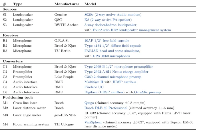
# Type Manufacturer Model
Sources
S1 Loudspeaker Genelec 8020c (2-way active studio monitor)
S2 Loudspeaker QSC K8 (2-way active PA speaker)
S3 Loudspeaker RWTH Aachen 3-way dodecahedron loudspeaker,
withFourAudio HD2 loudspeaker management system Receiver
R1 Microphone G.R.A.S. 40AF 1/2” free-field capsule R2 Microphone Bruel & Kjær Type 4134 1/2” diffuse-field capsule R3 Microphone TU Berlin FABIAN head and torso simulator,
withDPA 4060 microphones Converters
C1 Microphone Bruel & Kjær Type 2669-B 1/2” microphone preamplifier C2 Preamplifier Bruel & Kjær Type 2692-A-0I1 Nexus charge amplifier C3 Preamplifier Lake People C360 2-channel microphone preamp C4 Audio interface RME Multiface IIwithHDSP cardbus
C5 Audio Interface RME Fireface UC
C6 Audio Interfaces RME Digiface(HDSP cardbus) withOctaMic preamp Positioning tools
M1 Cross line laser Bosch Quigo(claimed accuracy±0.8 mm/m)
M2 Laser distance meter Bosch Bosch DLE 50 Professional(claimed accuracy±1.5 mm)
M3 Laser angle meter geo-FENNEL EL 832 (claimed accuracy±0.5◦, equipped with Hama LP-21 laser pointer)
M4 Room scanning system TH Cologne VariSphear(claimed accuracy±0.02◦, equipped with Topcon EM-30 laser distance meter)
Table 3: Hardware used for the acquisition of the BRAS. See Table2for a list of used hardware per scene.
Device Reference point
Genelec 8020c (loudspeaker)
Point on the front panel midway between the outmost position of the low/mid frequency driver and the tweeter
QSC-K8 (loudspeaker)
Point on the protective grid in front of the tweeter
Dodecahedron (loudspeaker)
Low-frequency unit: center of circular opening; Mid-frequency unit: center of sphere; High-frequency unit: center of sphere
B&K type 4134 G.R.A.S. 40AF (microphones)
Point on the center of the protective grid in front of the membrane FABIAN
(dummy head)
Interaural center, defined as the midpoint of the line that connects the entrances of the two ear channels
Table 4: Definition of the reference points that define the positions of the sources and receivers. The orienta- tion of the transducers is documented in the database separately for each scene.
average). A check for planarity of the major room sur- faces (walls, floor, ceiling) was done by fitting a plane through the points of each surface. Mean absolute de- viations in direction of the surface normal of 2.6 cm were corrected by moving the points on to the surface.
Maximum deviations of 6 cm and 8.5 cm occurred in two cases in the reverberation chamber (CR1) where the corner points were not clearly defined and for a wall that showed small irregularities. Since the rever- beration chamber only serves as the coupled volume for the main room of CR1, this outlier seems less rele- vant. In addition, the RMS Hausdorff distance between the non-planar and planar surfaces was calculated for the walls floor and ceiling using METRO [8], with an average across rooms of 7.8 mm and the largest differ- ence of 3.8 cm again found for the reverberation (CR1).
Afterwards, the 3D modeling software SketchUp was used to design the final room model based on the post- processed point clouds.
Due to the complexity of scene CR4, the initial room model was based on architectural drawings and vali- dated against a set of 15 manually measured distances between relevant points in the room (e.g. the height width and depth at different positions in the room).
Deviations between measured and initially modeled distances were smaller than 52 cm and 20 cm on av- erage, and the model was corrected according to the measurements by adjusting the position of the floor, ceiling and walls. In a final step, material names were assigned to each surface in the room models using SketchUp, and the positions and orientations of the sources/receivers were inserted.
The geometry acquisition aimed at obtaining a higher level of detail than the resolution of 50 cm typ- ically used for GA simulations [9, p. 176]. The mod-
els thus include structures that might have to be sim- plified depending on the need of the simulation algo- rithm. Nevertheless, not all details of the complex rooms (CR1–4) were captured, and the final models are accompanied by a list of model simplifications and pic- tures that show the omitted details (cf. Section2.1.1).
Not modeled were, for example, handrails and cable ducts with diameters of a couple of centimeters, stucco ornamentation, projections on walls with a depth of a couple of centimeters, and chandeliers.
The additional check of the positioning precision by means of onset detection could not be done for CR1–4, because i) the Genelec loudspeaker was not facing the receivers, and ii) the dodecahedron source consists of multiple drivers, which substantially widens the direct sound impulse and caused errors in the onset detection.
However, the positioning was done in analogy to scenes RS1 & 5–7 using lasers, and it is thus reasonable to assume that the positioning accuracy is comparable to that of scenes RS1 & 5–7.
3.2 Surface descriptions
As mentioned in the introduction, it is challenging to provide high precision boundary conditions for room acoustical simulations. For this purpose, absorption coefficients of the reference scenes RS1-7 were mea- sured in situ, whereas they were derived from a combi- nation of measurements and tabulated values of similar materials for the complex rooms CR1–4, where they can be considered as a best practice approximation.
In total, the database contains 28 surface materials, stored in 37 data files including absorption and scatter- ing coefficients in third octaves from 20 Hz to 20 kHz.
Multiple files are available for some materials providing data for different angles of incidence.
3.2.1 Absorption coefficients
Reference scenes. For RS1–7, three materi- als were used and described for different configura- tions. These include the floor tiles of the hemi ane- choic chamber, stone wool absorber tiles, and three medium density fiberboards (MDF) with a thickness of 12 mm (8.91 kg/m2) and 25 mm (15.53 kg/m2, and 18.56 kg/m2), which were used to build the reflecting and diffracting objects in RS1–7. An overview of all materials and the applied acquisition methods includ- ing the valid frequency ranges is shown in Table5.
Normal incidence absorption coefficients were mea- sured according to 10534-2 [10] using a circular impedance tube with a diameter of 2 inch. Transfer functions were determined for four microphone posi- tions with distances from the first to the second, third and fourth microphone of 17 mm, 110 mm and 510 mm, respectively. All transfer functions were measured by moving one probe microphone to the desired positions on the mid-axis of the circular tube. Crossover frequen- cies for the transfer functions between the first (H14)
Material
Absorption coefficient acquisition method (valid freq. range)
Scenes Medium
density fiberboard
ISO 10534-2, normal incidence (100 Hz to 4 kHz)
RS1–7
Stone wool absorber
ISO 10534-2, normal incidence (100 Hz to 4 kHz),
RS1–2
Stone wool absorber
Angle dependent in situ measurement (300 Hz to 15 kHz)
RS1–2
Wooden diffusor
Angle dependent in situ measurement, (500 Hz to 15 kHz)
RS1 Tiles of hemi
anechoic chamber
Estimated random incidence values (see text)
RS1, 5–7
Room surfaces (24 materials)
Estimated random incidence values (see text)
CR1–4
Table 5: Surface materials of the BRAS database in- dicating the applied absorption coefficient acquisition method and the scenes in which the corresponding ma- terials were used.
and the second microphone pair (H13), and between the second (H13) and the third microphone pair (H12), were defined at 900 Hz and 1200 Hz, respectively. The measurements are valid above 100 Hz due to the limited frequency range of the loudspeaker, and below 4 kHz due to the diameter of the tube [10].
Angle-dependent absorption coefficients of the stone wool absorber and the diffusor were determined using the setup and measurements of RS1. In the impulse response measurements of the rigid floor, the diffusor and the absorber, the reflection was isolated as de- scribed by Mommertz [11] for four φin – φout com- binations. This was done by a two-sided Hann win- dow (0.6 ms fade in, 1.8 ms fade out, cf. Fig. 4, top). The reflection factors were then obtained by spectral division, referencing the windowed impulse re- sponses of the absorber and diffusor to the rigid floor (cf. Fig.4, middle). The absorption coefficients were determined from the absolute value of the reflection factors, smoothed with a one-third octave sliding win- dow (cf. Fig.4, bottom). This was done for the sym- metric source/receiver setup (specular reflection) for the angles φin = φout = {30◦,45◦,60◦} based on the impulse responses of the omnidirectional receiver, and forφin = 45◦, φout = 32◦ based on the binaural data.
For other combinations of φin and φout, no measured data is provided, but can be processed from the pro- vided measured impulse responses of scene RS1. The lower frequency limit of this method differs for the two measured materials due to edge effects (cf. Table 5).
Above 15 kHz, minor differences of source, receiver, and probe positions affect the measured result. Miss-
10 15 20 25 30
t in ms 40
60 80 100
Amplitude in dB SPL
100 1k 10k 20k
f in Hz 90
100 110
Amplitude in dB SPL
100 1k 10k 20k
f in Hz 0.2
0.4 0.6 0.8 1
Absorption coeff.
Figure 4: Generation of the angle dependent absorp- tion coefficient for the example of the absorbing setup and anglesφin=φout = 30◦. Top: Windowed (black) and full length impulse response (gray) of the absorbing setup. Middle: Frequency responses of the absorbing (black) and rigid (gray) reflection calculated from the windowed impulse responses. Bottom: Unsmoothed (gray) and final (circles) absorption coefficients αob- tained after 3rd octave smoothing
ing values below and above the valid frequency ranges were linearly extrapolated or attributed from tabulated values of similar materials [9,12]. The absorption data of the stone wool absorber obtained in this way is con- sistent with other measurement results using ISO 354 and ISO 10534-2 for random-incidence and normal in- cidence, respectively, considering angle-dependent ef- fects such as an increase of absorption for an increasing angle of incidence.
The absorption of the tiles of the reflective floor of the hemi anechoic chamber (RS1, 5–7) can be described by an almost frequency independent absorption coeffi- cient with an average value of less than 0.02.
Complex rooms. For scenes CR1–4, several sur- faces were initially measured with a hand-held in situ device [13], consisting of a loudspeaker in a spherical enclosure and a combined sensor unit measuring sound pressure and particle velocity [14]. This method can deliver valid results for normal incidence if applied for porous absorbers in controlled scenarios, but faces sev- eral challenges otherwise. These include high uncer- tainties for reflective surfaces and repeated measure- ments as well as small and complex objects such as chairs. For these reasons the absorption data was de- rived from in-situ measurements whenever possible and attributed from material databases otherwise [9, 12]
(cf. Section 2.3). Less important materials and small
surfaces were disregarded, which lead to four, five, seven, and eight different materials for scenes CR1–4, respectively. Examples for left out surfaces are small doors far away from all source/receiver positions and stucco ornamentation. These sets of coefficients were termedinitial estimates.
To allow a comparison with the results of RR-I–III and the common practice of room acoustical simula- tion, a second set of fitted estimates is provided for the materials of CR1–4. These were fitted to the mea- sured reverberation times by multiplication with the ratio ¯α/¯α for each third octave band and scene, i.e., the same ratio was applied for all materials within a scene. ¯αdenotes the average absorption coefficient in CR1–4 calculated under the assumption of a diffuse sound field by solving the Eyring reverberation time for ¯α
TEyring= 0.161 V
−S ln(1−α) + 4mV¯ , (1) (V: room volume according to Appendix: Complex rooms; m: air attenuation [3]). The average absorp- tion coefficient of the initial estimates ¯αwas calculated using
α¯= 1 S
i
Siαi (2)
where the surface area S =
iSi occupied by each material was taken from the 3D room models.
3.2.2 Scattering coefficients
As GA based simulation algorithms commonly take into account non-specular reflections, the BRAS also includes random-incidence scattering coefficients for most materials. Although ISO 17497-1 [15] and ISO 17497-2 [16] describe standardized measurements of random-incidence scattering and directional diffu- sion, material samples in the required size could not be removed from the rooms. The scattering coefficients of the database were therefore estimated [17] based on the characteristic depth dchar [9] of the material in order to provide a transparent calculation model
s(f) = 0.5·
dchar
c/f , (3)
with c being the speed of sound andf the frequency.
As the scene geometries also contain large flat surfaces, the lower limit of s(f) was chosen as 0.05, the upper limit was set to 0.99. The structural depth of all mate- rials is listed in the corresponding material description files. The resulting scattering data for the 31 one-third octave center frequencies between 20 Hz and 20 kHz are provided for all materials, except for the wooden diffu- sor (RS1), as for this scenario, the modeling of scatter- ing effects of the diffusor is subject of the investigation.
4611.310.75308.5
Figure 5: Picture of the DSP driven 3-way dodecahe- dral speaker. Measures are given in cm. A detailed 3D model is contained in the database (cf. Section2.2.
3.3 Source and receiver descriptions
3.3.1 Source Directivities
The directivities of the Genelec 8020c, QSC K8, and the dodecahedral speaker were measured in the hemi- anechoic chamber at RWTH Aachen University on a 2×2 equi-angular top pole sampling grid (Fig. 3b, right) using exponential sweeps (16,384 samples≈0.4 s
@ 44.1 kHz sampling rate). The sweep length was suf- ficient to obtain a peak-to-tail SNR of approximately 80 dB (cf. Fig. 7). The dodecahedral speaker is a custom DSP driven 3-way system with a single low- frequency driver and mid/high-frequency units consist- ing of 12 speakers in spherical enclosures (cf. Fig.5).
The cross-over frequencies of 177 Hz and 1.42 kHz were chosen according to the upper cut-off frequency of the 125 Hz and 1 kHz octave bands. It was pre- ferred over commercially available 1-way systems be- cause the small high frequency drivers ensure smaller deviations from omnidirectionality than observed with conventional systems [18,19]
Due to mechanical restrictions, two different systems were used for rotating the transducers: The Genelec 8020c and the dodecahedral speaker were placed on a turntable that controlled the azimuth at a height of 2 m above the ground. The elevation was controlled
100 1k 10k 20k f in Hz
-5 0 5 0 5
Amplitude in dB
fc/kHz G/dB Q 0.811.09
1.713.18 4.987.01 15.1
-1.64.0 -1.02.6 -1.6-1.9 -5.8
10.0 2.2 1.8 2.5 3.2 7.1 2.8
Figure 6: Equalized on-axis magnitude response of the QSC-K8 speaker (black), equalization (gray), and equalizer settings (center frequency, gain, quality).
Q = fc/|f2−f1|, where f1, and f2 are the two fre- quencies with a magnitude of G/2 dB (midpoint dB gain definition of the bandwidth according to Bristow- Johnson (1994) [20].)
by an arm that was equipped with a G.R.A.S. 40AF half inch free-field microphone at a distance of 2 m from the speaker. To maintain a sufficient time de- lay between the direct sound and the floor reflection, the lower hemisphere of the loudspeaker directivities was measured after flipping them about the reference points (cf. Tab.4). For both hemispheres, an overlap- ping region of 4◦ below the equator was measured for validation. Differences in one-third octave bands be- tween repeated measurements were below 1 dB, except for some directions behind the Genelec 8020c with low emitted energy. Overall, mean absolute differences of 0.5 dB (SD 0.6 dB) were observed in the overlapping region for third octaves above 1 kHz. In case of the dodecahedral speaker, separate directivities were mea- sured for the mid-frequency and high-frequency unit, in both cases for the full physical setup of the 3-way system (cf. Fig. 5), each referenced to the center of the corresponding unit. The low-frequency unit was modeled omnidirectional because the wavelength at the upper cut-off frequency (1.94 m; 177 Hz) is more than four times larger than the enclosure (0.46 m high). The QSC K8 was rotated using the ELF loudspeaker mea- surement system (Four Audio) with the microphone placed flush with the floor of the hemi-anechoic cham- ber at a distance of 8 m. All equalizer settings of the speakers were disabled for reproducibility. Parametric equalizers were used, both in the directivity measure- ment and in the measurement of the BRIRs, to com- pensate the free-field on-axis frequency response of the QSC-K8 speaker within a tolerance of±3.5 dB to pro- vide an uncolored on-axis frequency response during auralization (cf. Fig.6and Section3.4.2).
The measurement distances were chosen in agree- ment with the far field criteriarlandrf l2/c[21, p. 102], where r is the measurement distance, l the acoustically effective source dimension (tweeter-to- woofer distances of 0.11 m and 0.3 m for the Genelec 8020c and QSC-K8, diameters of 0.3 m and 8.5 cm for the Dodecahedron mid and high frequency units),
f the upper frequency limit (16 kHz for the Gen- elec 8020c, QSC-K8, and Dodecahedron high frequency unit; 1.42 kHz for the Dodecahedron mid frequency unit), andc the speed of sound (343 m/s).
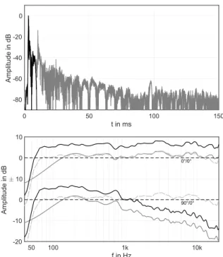
In post-processing, the common propagation delay was removed and a subsonic high-pass filter was ap- plied (4th order Butterworth -3 dB @ 30 Hz). Due to the different mechanical measurement setups and tem- poral behaviours, IRs were truncated to 9.5 ms (Gen- elec), 13.6 ms (dodecahedron), and 80 ms (QSC) to discard reflections by applying a 2 ms Hann window fade in/out (cf. Fig7). In case of the Genelec speaker, the truncation distorted the magnitude response be- low 200 Hz. To account for this, the magnitude spec- trum of a single on-axis measurement – done in the fully anechoic chamber at TU Berlin – was fitted to the truncated IRs by applying a linear fade between 200 Hz and 300 Hz in the frequency domain (gray lines in Fig.7). The phase response did not suffer from the truncation and was thus left unchanged, i.e., was taken from the truncated IRs. The substitution of only the magnitude response is similar to the combination of near-field and far-field loudspeaker measurements [22].
As a consequence, the final Genelec directivity is om- nidirectional below 200 Hz . Since the originally mea- sured data (before windowing) showed deviations from omnidirectionality of less than 1 dB below 200 Hz, this was neglected.
In a final step, separate spherical harmonics inter- polations (Eq. (3.26) and (3.31) in [23]) of the mag- nitude and unwrapped phase spectra with a spherical harmonics order of 20 were used to increase the spa- tial resolution and to harmonize the sampling grids, which differed across the systems used for the direc- tivity measurements. Differences before and after the interpolation were smaller than 0.4 dB below 10 kHz, and never exceeded 1 dB. The final data are available as impulse responses and complex one-third octave spec- tra on a 1◦×1◦ equal angle front pole sampling grid (cf. Fig.3a).
3.3.2 Receiver Directivies
Two types of receivers were used during the acqui- sition of the database. Impulse responses with om- nidirectional receivers were measured either with dif- fuse field or free field compensated half inch cap- sules, Br¨uel&Kjær type 4134 and G.R.A.S. 40AF, re- spectively, both using Br¨uel&Kjær 2669-B microphone preamplifiers. They are supposed to be modeled as omnidirectional receivers in the simulation.
The binaural impulse responses were measured with the FABIAN head and torso simulator, with acoustically measured head-related impulse responses (HRIRs) taken from the open access FABIAN database [24, 2]. It contains HRIRs for 11 different head-above-torso orientations (HATOs), i.e., head rotations to the left and right in steps of 10◦ covering the typical range of motion of ±50◦ [25]. To ensure
0 50 100 150 t in ms
-80 -60 -40 -20 0
Amplitude in dB
50 100 1k 10k
f in Hz -20
-10 0 10 0 10
Amplitude in dB
0°/0°
90°/0°
Figure 7: Processing of the Genelec 8020c directivity data. Top: Impulse response for the frontal direc- tion (0◦/0◦) before (gray) and after windowing (black).
Bottom: Final frequency responses after spherical har- monics processing (black) in front (0◦/0◦) and to the side (90◦/0◦). The measured directivity after window- ing (gray) and the single on-axis measurement that was used below 200 Hz (dashed) are given for validation.
Data are 12th octave smoothed to improve the visibil- ity.
that head movements can be auralized without per- ceivable degradation, HATOs with a resolution of 2◦ (threshold from [26]) were interpolated ([27], original phase, frequency domain, torso interpolation) using AKtools for Matlab [28]:
AKhrirInterpolation(A, E, HATO,
’measured sh’).
3.4 Impulse Responses
3.4.1 Omnidirectional Receivers
Impulse responses were measured using exponential sweeps (262,144 samples ≈ 6 s @ 44.1 kHz sampling rate) and averaged across four repeated measurements to increase the SNR. A high frequency amplitude re- duction that can occur when averaging room impulse responses was not observed [29], with deviations be- tween reverberation times (T20@ 4 kHz and 8 kHz) of averaged and single impulse responses always smaller than 1.4% and 0.4% on average. The microphones were always oriented towards the current sound source posi- tion, corresponding to the 0◦direction as defined by the manufacturers. The input measurement chain was cal- ibrated using a B&K Type 4231 sound calibrator, and
the input channels of the interfaces were calibrated us- ing a voltage calibrator. The input-to-output latency was removed according to a loopback measurement.
To cut the impulse responses to the length defined in the scene description, the last 1024 samples were faded out using a one-sided Hann window. Details about the hardware used for each scene and the final impulse re- sponse lengths can be found in Table3, Appendix A, andAppendix B.
Reference scenes. RS1–7 were measured with a G.R.A.S. 40AF free field compensated microphone cap- sule and the Genelec 8020c.
Complex rooms. CR1–4 were measured with a diffuse field compensated B&K 4134 capsule, the Gen- elec 8020c, and the dodecahedral speaker. For CR2–4, source and receiver positions and characteristics were chosen according to the requirements of ISO-3382-1 [30]. The measured IRs using the omnidirectional do- decahedron source thus allow the processing of most of the room acoustical parameters. A Matlab script for calculating C80, D50, EDT or T20 (among other pa- rameters) using the ita roomacoustics method of the ITA-Toolbox [4] is part of the BRAS.
3.4.2 Binaural Receiver
BRIRs were measured with the FABIAN head and torso simulator [31], the Genelec 8020c, and the QSC- K8 using swept sines and spectral deconvolution. The sweep length and level was adjusted to obtain SNRs of about 90 dB for a source in front of FABIAN, except at RS5, where a reduced SNR of 70 dB is due to the energy loss caused by the blocked direct sound path.
FABIAN is equipped with DPA 4060 miniature elec- tret condenser microphones located at the blocked ear channel entrances, and a computer controllable neck joint (Amtec Robotics PW-070, precision±0.02◦) that was used to obtain BRIRs for head orientations of±44◦ in steps of 2◦ to cover a typical range of motion, and allow for an artifact free dynamic auralization of head rotations [25,26].
In post-processing, the smallest common propaga- tion delay was removed from all BRIRs to minimize the latency in auralizations. This was done separately for each scene to assure that propagation delay differences between loudspeaker positions and HATOs remained as they were. A band pass filter was applied to suppress noise (4th order Butterworth, -3 dB @ 50 Hz/20 kHz). The on-axis magnitude response of FABIAN’s DPA microphones was removed to provide an uncolored on-axis frequency response for auralization by applying minimum phase inverse filters with a length of 128 samples. Afterwards the impulse responses were truncated at the position where the noise floor became visible and squared sine fades were applied to avoid discontinuities at the start and beginning. In a last step, the BRIRs were normalized using a single gain factor per scene, thus maintaining interaural level differences and relative level differences
between BRIRs for different speakers and HATOs.
To obtain the gain factor, the BRIR measured with the speaker closest to FABIAN (with neutral head orientation) was averaged between 300 Hz and 1 kHz and across the left and right ear using AKtools [28]:
[∼,∼,gain] = AKnormalize(brir l r, ’abs’,
’mean’, ’mean’, 1, [300 1000]);
For the audio content provided in the database (ane- choic string quartet, see Section 2.4) the bandwidth is sufficient, with C2 being the lowest playable note on a Cello with a fundamental frequency of 65 Hz. For other stimuli, the 50 Hz limit could indeed be a restriction.
In these cases, the the same band-pass filter should be applied to the simulation.
Reference scenes. In RS1, 3, and 5 BRIRs were measured for selected positions of the Genelec 8020c.
Complex rooms. BRIRs were measured for se- lected positions of the Genelec 8020c in CR1. In CR2–
4 a single receiver position was used and the QSC-K8 speaker was set up at five different positions to mimic a string quartet with a singer. For this purpose, the speakers were arranged in a hemi-circle with a radius of 1.5 m at positions of ±90◦ (1st violin, cello) and
±30◦(2nd violin, viola), and tweeter heights of 103 cm (violins, viola) and 81 cm (cello). To realize the tilt- ing and tweeter heights, the speakers were placed on a chair on top of a box (flight case filled with a layer of porous absorbers). A 3D model of the setup includ- ing the box, chair and loudspeaker is contained in the database (cf. Section 2.1.1). The speaker that mim- icked the singer was placed on a stand in the center of the semi-circle with a tweeter height of 1.5 m. Except for the center, the speakers were rotated and tilted un- til the tweeter pointed towards FABIAN’s head (the position and orientation of the speaker was identical for all measured head orientations). BRIRs for the five source positions were measured one after another to avoid reflections from other speakers. Parametric equalizers were used to provide an uncolored on-axis frequency response of the QSC-K8 for auralization as described in section 3.3.1.
Acknowledgements
We would like to thank Thomas Maintz, Rob Opdam, Philipp Eschbach, Ingo Witew, Johannes Klein, and the workshop of the Institute of Technical Acoustics at RWTH Aachen University; Hannes Helmholtz, and Omid Kokabi from the Audio Communication Group at TU Berlin for assistance during the compilation of the BRAS database, and Oliver Strauch for measuring the directivity of the QSC-K8.
References
[1] AES Standards Comittee, AES69-2015: AES standard for file exchange - Spatial acoustic data file format. Audio Engineering Society, Inc., 2015.
[2] F. Brinkmann, A. Lindau, S. Weinzierl, G. Geissler, S. van de Par, M. M¨uller-Trapet, R. Opdam, and M. Vorl¨ander, “The FABIAN head-related transfer function data base,” DOI:
10.14279/depositonce-5718.3, Feb. 2017.
[3] H. Kuttruff,Room acoustics, 5th ed. Oxford, UK:
Spon Press, 2009.
[4] M. Berzborn, R. Bomhardt, J. Klein, J.-G.
Richter, and M. Vorl¨ander, “The ITA-Toolbox:
An open source MATLAB toolbox for acous- tic measurements and signal processing,” in Fortschritte der Akustik – DAGA 2017, Kiel, Ger- many, Mar. 2017, pp. 222–225.
[5] S. M¨uller and P. Massarani, “Transfer function measurement with sweeps. directors cut includ- ing previously unreleased material and some cor- rections,” J. Audio Eng. Soc. (Original release), vol. 49, no. 6, pp. 443–471, Jun. 2001.
[6] A. Andreopoulou and B. F. G. Katz, “Identifi- cation of perceptually relevant methods of inter- aural time difference estimation,”J. Acoust. Soc.
Am., vol. 142, no. 2, pp. 588–598, Aug. 2017.
[7] B. Bernsch¨utz, “A spherical far field HRIR/HRTF compilation of the Neumann KU 100,” in AIA- DAGA 2013, International Conference on Acous- tics, Merano, Italy, Mar. 2013, pp. 592–595.
[8] P. Cignoni, C. Rocchini, and R. Scopigno, “Metro:
Measuring error on simplified surfaces,”Computer Graphics Forum, vol. 17, no. 2, pp. 167–174, 1998.
[9] M. Vorl¨ander, Auralization. Fundamentals of acoustics, modelling, simulation, algorithms and acoustic virtual reality, 1st ed. Berlin, Heidel- berg, Germany: Springer, 2008.
[10] ISO 10534-2, Determination of sound absorption coefficient and impedance in impedance tubes – Part 2: Transfer-function method. Geneva, Switzerland: International Organization for Stan- dards, Nov. 1998.
[11] E. Mommertz, “Angle-dependent in-situ measure- ments of reflection coefficients using a subtraction technique,”Applied Acoustics, vol. 46, no. 3, pp.
251 – 263, 1995, building Acoustics.
[12] Physikalisch-Technische Bundesanstalt (PTB),
“Tabularized absortion and scattering values,”
https://www.ptb.de/cms/fileadmin/internet/
fachabteilungen/abteilung 1/1.6 schall/1.63/
abstab wf.zip(last checked Mar. 2019), 2012.
[13] M. M¨uller-Trapet, P. Dietrich, M. Aretz, J. van Gemmeren, and M. Vorl¨ander, “On the in situ impedance measurement with pu-probes — Simu- lation of the measurement setup,”J. Acoust. Soc.
Am., vol. 134, no. 2, pp. 1082–1089, Aug. 2013.
[14] E. Tijs, “Study and development of an in situ acoustic absorption measurement method,” Ph.D.
dissertation, University of Twente, Enschede, The Netherlands, Apr. 2013.
[15] ISO 17497-1, Sound-scattering properties of sur- faces. Part 1: Measurement of the random- incidence scattering coefficient in a reverberation room. Geneva, Switzerland: International Orga- nization for Standards, May 2004.
[16] ISO 17497-2, Sound-scattering properties of sur- faces. Part 2: Measurement of the directional dif- fusion coefficient in a free field. Geneva, Switzer- land: International Organization for Standards, May 2012.
[17] B. N. J. Postma and B. F. G. Katz, “Creation and calibration method of acoustical models for historic virtual reality auralizations,” Virtual Re- ality, vol. 19, pp. 161–180, Sep. 2015.
[18] G. Behler and M. Vorl¨ander, “An active loudspeaker point source for the measurement of high quality wide band room impulse responses,”
in Proceedings of the Institute of Acoustics – Auditorium Acoustics 2018, vol. 40, no. 3.
Hamburg, Germany: Instiute of Acoustics, 2018, pp. 435–446. [Online]. Available: https:
//www.dega-akustik.de/fileadmin/dega-akustik.
de/DEGA/aktuelles/IOA AA Program.pdf [19] T. W. Leishman, S. Rollins, and H. M. Smith,
“An experimental evaluation of regular polyhe- dron loudspeakers as omnidirectional sources of sound,”J. Acoust. Soc. Am., vol. 120, no. 3, pp.
1411–1422, Sep. 2006.
[20] R. Bristow-Johnson, “The equivalence of various methods of computing biquad coefficients for au- dio parametric equalizers,” in 97th AES Conven- tion, Preprint, San Francisco, USA, Nov. 1994.
[21] M. M¨oser, Engineering acoustics: An Introduc- tion to noise control, 2nd ed. Berlin Heidelberg:
Springer, 2009.
[22] D. B. Keele Jr., “Low-frequency loudspeaker as- sessment by nearfield sound-pressure measure- ment,”J. Audio Eng. Soc., vol. 22, no. 3, pp. 154–
162, Apr. 1974.
[23] B. Rafaely, Fundamentals of spherical array pro- cessing, 1st ed. Berlin, Heidelberg, Germany:
Springer, 2015.
[24] F. Brinkmann, A. Lindau, S. Weinzierl, S. v. d. Par, M. M¨uller-Trapet, R. Opdam, and M. Vorl¨ander, “A high resolution and full- spherical head-related transfer function database for different head-above-torso orientations,” J.
Audio Eng. Soc, vol. 65, no. 10, pp. 841–848, Oct.
2017.
[25] W. R. Thurlow, J. W. Mangels, and P. S. Runge,
“Head movements during sound localization,” J.
Acoust. Soc. Am., vol. 42, no. 2, pp. 489–493, 1967.
[26] A. Lindau and S. Weinzierl, “On the spatial res- olution of virtual acoustic environments for head movements on horizontal, vertical and lateral di- rection,” inEAA Symposium on Auralization, Es- poo, Finland, Jun. 2009.
[27] F. Brinkmann, R. Roden, A. Lindau, and S. Weinzierl, “Audibility and interpolation of head-above-torso orientation in binaural technol- ogy,”IEEE J. Sel. Topics Signal Process., vol. 9, no. 5, pp. 931–942, Aug. 2015.
[28] F. Brinkmann and S. Weinzierl, “AKtools – An open software toolbox for signal acquisition, pro- cessing, and inspection in acoustics,” in 142nd AES Convention, Convention e-Brief 309, Berlin, Germany, May 2017.
[29] B. N. J. Postma and B. F. G. Katz, “Correction method for averaging slowly time-variant room impulse response measurements,” J. Acoust. Soc.
Am., vol. 140, no. 1, pp. EL38–EL43, 2016.
[30] ISO 3382-1,Measurement of room acoustic param- eters – Part 1: Performance spaces. Geneva, Switzerland: International Organization for Stan- dards, 2009.
[31] A. Lindau, T. Hohn, and S. Weinzierl, “Binaural resynthesis for comparative studies of acoustical environments,” in 122th AES Convention, Con- vention Paper 7032, Vienna, Austria, May 2007.
[32] F. Brinkmann, M. Dinakaran, R. Pelzer, P. Grosche, D. Voss, and S. Weinzierl, “A cross- evaluated database of measured and simulated HRTFs including 3D head meshes, anthropomet- ric features, and headphone impulse responses,”
J. Audio Eng. Soc. (Engineering Report), vol. 67, no. 9, pp. 705–718, Sep. 2019.
[33] L. Asp¨ock, F. Brinkmann, D. Ackerman, S. Weinzierl, and M. Vorl¨ander, “GRAS – Ground Truth for Room Acoustical Simulation,” DOI:
10.14279/depositonce-6726, Mar. 2018.
[34] ——, “BRAS – Benchmark for Room Acoustical Simulation,” DOI: 10.14279/depositonce-6726.2, May 2019.
[35] ——, “BRAS – Benchmark for Room Acoustical Simulation,” DOI: 10.14279/depositonce-6726.3, Apr. 2020.
BRAS: Reference scenes
RS1: Simple reflection (infinite plate)
Short description: Simple reflection on three different (infinite) surfaces: Hard floor of hemi anechoic chamber, RockFon absorber and medium density fiber- board (MDF) diffusor. Monaural impulse responses for three loud- speaker positions and angles (30◦,45◦, 60◦) and three microphone positions. Binaural impulse responses for one loudspeaker position and one receiver position.
Room: Hemi anechoic chamber RWTH Aachen (V = 296 m3,flow= 100 Hz)
Temperature: 20.3◦C Humidity: 41.5 % Sampling rate: 44100 Hz
Scene geometry: RS1 RIR Floor.skp RS1 RIR Absorber.skp RS1 RIR Diffusor.skp RS1 BRIR Floor.skp RS1 BRIR Absorber.skp RS1 BRIR Diffusor.skp
Output IRs: 29 RIRs; 3 BRIR sets (11,025 samples duration)
Comment(s): For a more detailed description of the reflecting objects, see *.skp files in the folderAdditionalSceneDescription.