Probabilistic Programming: Applications of Martingales beyond Reachability

Author:

Thomas Haas

Advisor:

Prof. Dr. rer. nat. Roland Meyer

Institute of Theoretical Computer Science

Institute of Theoretical Computer Science Technische Universität Braunschweig

Germany

October 16, 2019

neural networks, randomized incremental constructions are found in the area of compu- tational geometry and Markov decision processes are a frequently used model in control theory. These stochastic aspects are also found in probabilistic programming, an extension of classical programming. Along with programming comes the natural arising problem of verification of programs, that is, the problem of deciding certain properties about pro- grams. Stochastic systems are much harder to verify and deciding qualitative properties such as safety and liveness requires more care. Unlike their deterministic counterpart, stochastic systems can also be analyzed in a quantitative manner by finding or approx- imating the probability that the system has certain properties. This thesis aims to give an overview over so called martingale-based methods which can be used to verify qualita- tive properties such as almost sure termination, but also to compute quantitative bounds like reachability probabilities. The models under consideration are probabilistic programs with nondeterminism. We look at the theory of martingale-based verification from two viewpoints, the probabilistic viewpoint via martingale theory and the order-theoretic view- point via fixed-point theory. We show the strong similarity between both viewpoints by redeveloping various martingale-based methods in both frameworks. These include mar- tingales for deciding almost sure reachability, but also martingales for bounding reacha- bility and recurrence probabilities. Lastly, we explain the idea of template-based synthesis to automatically find various martingales for program verification by using optimization techniques. Linear and polynomial templates are considered and experiments are done for the former. The results show that while linear template synthesis is a sound technique, it tends to give trivial or very bad approximations of probability bounds in many cases.

In contrast, for establishing the quantitative property of positive almost sure termination,

even linear templates can be useful.

declare that I have not submitted this thesis at any other institution in order to obtain a degree.

Date Signature

1 Introduction 1

2 Background 5

2.1 Probability Theory . . . . 5

2.1.1 Measurability . . . . 7

2.1.2 Martingale Theory . . . . 16

2.2 Order Theory . . . 22

3 Martingale-based Program Verification 25 3.1 Probabilistic programming . . . . 25

3.1.1 Programming Languages APP and PPP . . . . 25

3.1.2 Semantics of probabilistic programs . . . . 27

3.2 Application of Martingales . . . . 31

3.2.1 Additive Ranking Supermartingales . . . . 37

3.2.2 Ranking Supermartingales for Higher Order Moments . . . 46

3.2.3 Nonnegative Repulsing Supermartingales . . . . 51

3.2.4 Nonnegative Repulsing δ -Supermartingales . . . . 57

3.2.5 γ-scaled Submartingales . . . . 59

3.2.6 Martingales for Recurrence . . . 64

4 Template-based Synthesis 71 4.1 Linear Templates . . . . 71

4.2 Polynomial Templates . . . . 78

4.3 Experiments . . . . 81

5 Related Work 85

6 Conclusion 87

7 Future Work 89

3.3 Example: Probabilistic invariants . . . . 56

3.4 Example: Upper recurrence incompleteness . . . 66

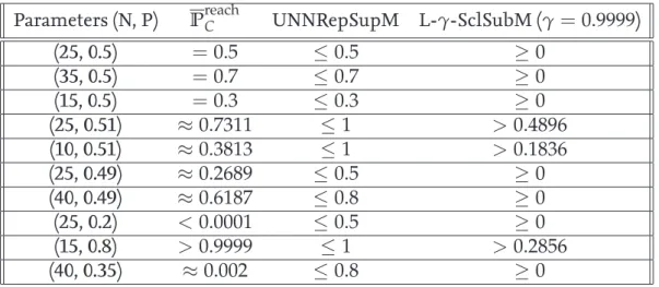
4.1 1d Random Walk . . . 82

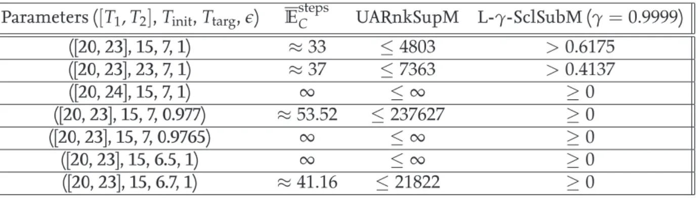
4.2 Refrigerator cooling system . . . . 83

List of Tables 4.1 Probability bounds for 1d-Random Walk . . . 82

4.2 Expected cooling time . . . 84

to describe them, but the most well-known and powerful ones include Turing machines and standard computer programs written in a programming language such as C, Java or Haskell. These systems are sequential, that is, they start from some starting state and then evolve through repeated transitions to successor states. The state space may be described as a set S and the evolution as a sequence of states S

, the runs of the system. An often asked question is whether the runs of a given program exhibit a certain property such as guaranteed termination, safety or liveliness. This decision of program properties is known as verification. Termination, however, is known to be an undecidable property since com- puter programs are known to be theoretically as powerful as Turing machines for which the so called Halting problem is undecidable. So instead of looking at arbitrary, unrestricted systems, more practical approaches have been adopted. One is to restrict the system, such as the memory size of a program or the allowed actions of the system. While these restric- tions can make many problems solvable, real life software may or may not adhere to any of the restricted models.

Another approach to deal with these kind of problems is to forgo the need to find an exact solution but to settle with incomplete but sound methods such as system behavior approximations. A common technique used to prove termination in term-rewriting sys- tems is by finding a well-ordering on the terms which decreases as rewriting rules are ap- plied. If such an ordering exists, then only finitely many rewrites can be performed before the system eventually can not perform any more rewrites[1, 2]. For deterministic programs, termination can be shown by finding so called ranking functions[3]. A ranking function can be seen as a kind of potential which decreases as the system evolves and guarantees that the system terminates as soon the potential goes below a certain threshold. In this sense, it induces a well-ordering on the state space of the system. A ranking function f roughly satisfies two properties:

1. f ( s ) ≥ ^f ( s

) + 1 for all transitions s → ^s

^,

2. f ( s ) ≤ b = ⇒ s is terminating state (where b is some threshold value)

Intuitively, the function assigns to each state the distance towards the terminating state and since it decreases over time (over transitions), it witnesses the fact that the system gets closer to termination as time progresses. A similar idea is used in systems modeled by ordinary differential equations (ODEs) where stability can be shown using so called Lya- punov functions [4, 5]. In either case, a system may be stable or may be terminating but a ranking function to witness it might not exist or might not be computable. Hence, finding a ranking function is generally a sound but incomplete method.

Another type of system where this approach is adopted are stochastic systems such as

probabilistic rewriting systems[6, 7] and probabilistic programs. A probabilistic program,

in contrast to usual deterministic programs, can also model stochastic behavior by e.g.

sampling from distributions or branching in a probabilistic manner. Thus, probabilis- tic programs exhibit strictly more behavior than their deterministic counterpart, making problems such as sure termination even harder to handle. Concretely, the notion of ter- mination is replaced by the notion of almost sure termination, asking whether the system terminates with probability 1.

Ranking functions as described before are insufficient to witness almost sure termina- tion. The problem is that many stochastic systems, even when terminating almost surely, occasionally move away from the terminating state caused by their stochastic behavior.

So instead of a function which witnesses the systems guaranteed evolution towards ter- mination along all transitions, a function which witnesses an expected evolution towards termination is more appropriate. For this purpose, so called probabilistic ranking func- tions (also sometimes called Lyapunov-style ranking functions) are used[8, 9, 10, 8, 11, 12].

Intuitively, they model the expected distance (expected number of steps/transitions) to the terminating state instead of the real distance.

1. f ( s ) ≥ E

( f ( s

) | s → s

) + 1 for all states s,

2. f ( s ) ≤ b = ⇒ s is terminating state (where b is some threshold value)

These probabilistic ranking functions turn out to have supermartingale behavior, which is a special kind of behavior of stochastic processes whose expected value is non-increasing over time. This allows the analysis via martingale theory and makes so called martin- gale concentration inequalities like AzumaHoeffding’s inequality applicable, giving certain bounds on the systems stochastic evolution.

Instead of looking at the termination problem in a qualitative, boolean way, the notion of termination probabilities becomes also available. Obviously, determining the exact prob- abilities encompasses the Halting problem for deterministic systems, making it generally undecidable. However, the problem of computing probabilities as real values allows a natu- ral relaxation, namely, approximation instead of exact computation. Probabilistic ranking functions are not directly applicable in this quantitative setting, but it turns out that the underlying notion of supermartingales (and also submartingales) is able to be extended to witness probability bounds. Difference-bounded repulsing supermartingales are a vari- ation of supermartingale processes that are capable of overapproximating the termina- tion or reachability probability, that is, they give quantitative bounds instead of qualitative assertions[12, 13]. These make use Azuma-Hoeffding’s inequality to derive their bounds.

The goal of this thesis is to give a solid understanding on how martingale-based methods can be used to tackle problems such as deciding (almost sure) termination of probabilistic programs, or finding bounds on the termination probability. Furthermore, they can also be used in a variety of other problems such as reachability, bounded reachability and tail reachability. We consider various different notions of martingales for different purposes such as

Additive ranking supermartingales for almost sure reachability[12, 13]

Higher order ranking supermartingales for bounding tail probabilities[14]

Nonnegative repulsing supermartingales for overapproximation of reachability prob- abilities [11, 13]

Nonnegative repulsing δ-supermartingales for overapproximation of bounded reach- ability probabilities[11]

γ-Scaled submartingles for underapproximation of reachability probabilities[11, 15]

A combination of super- and submartingale for recurrence probabilities

We develop the necessary theory from two different viewpoints, namely, once from the viewpoint of probabilistic martingale theory and once from the viewpoint of fixed point theory. From the former one, we derive soundness and completeness results by using the well-known Optional Stopping Theorem for martingales. We remark that we do not use any martingale concentration inequalities at all and solely rely on the Optional Stopping The- orem. From the fixed point theoretic point of view we derive the same results in a purely fixed point theoretic manner and establish the connection between martingales and fixed points. The extensive use of fixed point theory in this probabilistic martingale setting has recently been made by Takisaka et al.[11] and Kura et al.[14]. We build upon their work and extend it by providing the link between the commonly used pure martingale theoretic ap- proaches and their new fixed point theoretic approaches. Our notation is in the remainder of this work is heavily influenced by Takisaka’s and Kura’s work.

Our setting is probabilistic programs with nondeterminism; an extension of probabilistic programs with nondeterministic assignments and branchings. In the presence of nonde- terminism, the goal is to analyze the program under angelic and demonic behavior, i.e. to give probability bounds for the worst case and best case behaviors.

Martingale methods are applicable to infinite state systems such as those induced by probabilistic programs and in some cases even when non-deterministic behavior is present.

Remarkably, martingales are effective in the sense that they can be computed - under some restrictions - automatically using template-based optimization[12, 13, 11, 14]. We give a sim- ple description on how linear and polynomial templates can be used to compute martin- gales automatically via linear programming (LP) or semi-definite programming (SDP) and apply the linear template method experimentally.

Remark. For ease of presentation, the word martingale is often used to include the notions of supermartingales and submartingales although they are technically no martingales in the formal sense. In fact, none of the presented methods in this thesis use a strict martin- gale but always one of its relaxations.

The thesis is structured as follows:

1. Chapter 2 revises the basic theories of probability, measurability and martingales in Section 2.1. Section 2.2 revises order theory with a focus on lattices and fixed points.

2. Chapter 3 presents the main theory of this thesis showing how martingale-based

methods can be used in program verification. Section 3.1 introduces probabilistic

programs (with nondeterminism) syntactically and gives their semantics in terms

of probabilistic control flow graphs (pCFGs) and Markov decision processes (MDPs).

Section 3.2 introduces different concrete super- and submartingales which have been used to verify programs. Each type of martingale has its own dedicated subsection.

3. Chapter 4 explains how different martingales can be automatically synthesized using

template based optimization. Section 4.1 shows that martingale constraints for lin-

ear templates can be reduced to a linear programming problem. Section 4.2 shows

that polynomial template synthesis also works by using semidefinite programming

instead. Lastly, Section 4.3 demonstrates linear template-based synthesis by applying

it to various programs.

explicit focus on their specialized theories of martingales, measurability and fixed points.

Both of these theories are fundamental, and hence, crucial to the understanding of the re- mainder of this thesis. If the reader is familiar with these topics he may directly skip to Chapter 3 and come back to this chapter when necessary.

2.1 Probability Theory

This section revises the basics of probabilistic theory needed to understand the main con- tent of this paper. A special focus lies on measure theory and martingale theory which both are presented in their own subsections.

Definition 2.1.1 (Probability space). A probability space is a triple ( _Ω, F , µ ) consisting of 1. a set Ω called the sample space,

2. a family F ⊆ P ( _Ω ) of subsets of Ω forming a σ -Algebra, 3. a probability measure µ : F → [ 0, 1 ] .

The elements of F ^{are called} measurable sets, measurable events or simply just events. A set E which is not contained in F ^{is called} non-measurable. A σ-Algebra, in short, is a family of subsets which contains the whole space Ω and is closed under countable unions, countable intersections and complements. The probability measure µ simply assigns to each event the probability that that event occurs. It does so in a reasonable manner, given by the following axioms:

µ ( _Ω ) = 1, µ ( ^∪

i∈N

E

) = _∑

i∈N

µ ( E

) for countable collections of disjoint events E

.

The second property of µ is also called σ-additivity or countable additivity. It is easy to see that µ is monotone, i.e. µ ( A ) ≤ µ ( B ) for A ⊆ B. The reason why one restricts to a subset F ⊆ P ( _Ω ) of measurable events is discussed in Subsection 2.1.1 in more detail.

Broadly speaking, it is by no means easy to assign probabilities to arbitrary subsets of Ω because of rather complicated, pathological subsets (e.g. the Vitali sets in R). The definition of σ -Algebra and measurability is also discussed there.

Definition 2.1.2 (Random variable). A random variable X : Ω → Y is a measurable func- tion

between the probability space ( _Ω, F , µ ) and the measurable space ( Y, Σ ) .

1Measurability is defined in the following subsection

In most cases the target measurable space is ( _R, B ( _R )) or ( _R, B ( _R )) where B ^denotes the Borel σ-Algebra and R = _R ∪ {± ∞ } the extended reals, then X is called a (extended) real-valued random variable. The probability measure µ on ( _Ω, F ) defines a push-forward measure µ

: Σ → [ 0, 1 ] on ( Y, Σ ) by assigning to each S ∈ Σ the probability

µ

( S ) : = Pr ( X ∈ ^S ) = _µ ( { ω ∈ Ω | ^X ( _ω ) ∈ ^S } ) = _µ ( X

( S )) . For real-valued random variables the concept of integration is definable.

Definition 2.1.3 (Integration). Let X : Ω → [ 0, ∞ ] be a nonnegative, real-valued random variable. Then the integral of X with respect to a measure µ can be defined as

∫

Ω

Xdµ =

∫

Ω

X ( ω ) µ ( dω ) : = sup { ∑

i

inf { ^X ( _ω ) | ω ∈ ^A

} µ ( A

) | { ^A

} is a finite partition of Ω } ^. X is said to be integrable if ∫

Ω

Xdµ < _∞ holds.

This definition may be extended to real-valued random variables X : Ω → R by splitting X into its positive and negative parts and integrating them separately:

∫

Ω

Xdµ : =

∫

Ω

X

dµ − ^∫

Ω

X

dµ,

where X

: = max { 0, X } and X

: = max { 0, − X } . This integral is only defined if either of the right-hand side integrals takes a finite value. X is then said to be integrable if | X | ^: = X

+ X

is integrable, that is, both integrals are finite.

Using the push-forward measure µ

of a random variable X : Ω → R one may alterna- tively integrate over R instead of Ω via the identity

∫

Ω

Xdµ =

∫

R

xdµ

=

∫

R

xµ

( dx ) .

An important theorem related to integration is the so called Monotone Convergence Theo- rem which shows the exchangability of taking the monotone limit and integration.

Theorem 2.1.1 (Monotone Convergence Theorem). [16, Theorem 2.146] Let { ^X

}

be a monotonically increasing sequence of nonnegative random variables that converges point-wise to a random variable X. Then the limit operation and the integration operation commute:

n

lim

∫

X

dµ =

∫

n

lim

X

dµ =

∫ Xdµ.

Definition 2.1.4 (Moments). The k-th moment of a real-valued random variable X is given by

E ( X

) : =

∫

Ω

X

dµ.

The first moment E ( X ) is also called the expectation of X. The second moment of the random variable ( X − E ( X )) is also known as the variance of X.

In Section 3.1 the notion of probabilistic programs over real-valued variables is introduced.

The objects of interest are the possible runs of the system, that is, the sample space is the set of all sequences of program configurations. A typical quantity to analyze is the expected termination time. The termination time may be given by a random variable T which assigns to each run the time it takes to enter a terminating state or ∞ if it does not terminate, then the problem of deciding positive

almost sure termination is reduced to computing E ( T ) .

2.1.1 Measurability

Many results about measurability in this section apply to general measurable spaces and are not unique to probability spaces. Accordingly, most results about measurability are stated with respect to arbitrary measurable spaces.

The goal of measure theory is to measure objects (subsets) and assign them some kind of real value indicating mass, size or probability. Consider for example the 2d-plane R

. A reasonable measure in this setting is the measure of area. For many geometric objects like rectangles, disks or arbitrary polygons, elementary formulas are known which give the area of such objects. An immediately arising question is how one measures more complex ob- jects or even arbitrary subsets of for example R

. Measure theory tries to give an answer to this question. It turns out that assigning lengths, areas or volumes to arbitrary subsets of R

is not easy at all. Indeed, the well known Vitali sets discovered by Giuseppe Vitali give an example of subsets of R which cannot be assigned a geometric length in a consis- tent manner. Hence, the Vitali sets are said to be non-measurable. Another example is the Banach-Tarski paradox which shows that a ball can be decomposed into multiple parts and then reassembled into two balls of the same size as the original, effectively doubling the original ball. This decomposition is non-trivial and needs the Axiom of Choice (so do the Vitali sets). The Banach-Tarski paradox shows that the parts obtained in the decomposition are in a sense so complexly or oddly shaped that the concept of geometric size fails to apply.

In both cases, it was assumed that a reasonable geometric measure shall be invariant under translation and rotation. This shows that under these simple geometric conditions we are forced to somehow restrict the objects to be measured. These kind of problems also arise when trying to assign a probability to events instead of a geometric size to geometric object.

To circumvent such problems, instead of trying to measure arbitrary subsets, one restricts to a family of so called measurable subsets which are given in the form of a σ-Algebra.

Definition 2.1.5 (σ-Algebra). A σ-Algebra Σ of a set X is a family of subsets which contains the whole set X ∈ Σ,

is closed under countable unions: ^∪

A

∈ Σ for A

∈ Σ, and is closed under complementation: A ∈ Σ = ⇒ ( X \ A ) ∈ Σ.

2Positive a.s. termination means finite termination time, while (standard) a.s. termination refers to the probability of termination to be1. The former implies the latter, but not vice versa.

The empty set ∅ = X \ ^X ∈ Σ is also contained in Σ and by De Morgan’s laws, Σ is also closed under countable intersections.

Intuitively, one expects that if some finite set of objects are measurable then surely their union, intersection and complement can be measured as well. By applying limit proce- dures, this concept of measurability can then be extended to countable unions and inter- sections as well. This intuition leads to the idea to actually construct a σ-Algebra from a set of simple measurable objects. Assume that there is a family of subsets for which it is easy to define some kind of measure, e.g. consider the real line R and its open intervals ( a, b ) . It is straightforward to assign a size to intervals ( a, b ) , namely the length b − a. Starting from these open intervals, one can construct a σ-Algebra by finding the closure with respect to countable unions and complements. This specific σ -Algebra which is generated from the open intervals is the so called Borel σ-Algebra. It will be formally introduced later in this section. Although defining this generated σ-Algebra is straightforward, extending the mea- sure on the simple intervals to the whole σ -Algebra is not. Some more assumptions on the measure and the generating set are needed to make it work as expected.

Borel σ-Algebras are the most important σ-Algebras in measure theory, and the most commonly analyzed σ -Algebras are either the Borel σ -Algebras themselves or some larger σ-Algebra containing it. Before further going into this specific σ-Algebra, we first formalize the previously mentioned idea of constructing σ-Algebras.

Definition 2.1.6 (Generated σ -Algebra). Let A be a family of subsets of a ground set X.

Define σ ( A ) to be the smallest σ-Algebra containing A . It is formally given by σ ( A ) = ^∩

A⊆Σ

Σ

where the intersection ranges over all possible σ-Algebras Σ containing A . This intersec- tion is well defined, because the family of σ -Algebras is closed under arbitrary intersections and it is nonempty because it contains a largest element P ( X ) which always contains A ^. Remark. A pre-measure defined on a family of subsets can in generally not be extended to a measure on its generated σ -Algebra. The generating set has to satisfy some extra properties in order for this to work. Carathéodory’s extension theorem[17] states that if the generating set forms a ring, then the pre-measure on this ring can be extended to a measure on the generated σ -Algebra. If the pre-measure is σ -additive, then this extension is unique.

Now we are ready to define the object of interest, namely measurable spaces.

Definition 2.1.7 (Measurable space). A measurable space is a tuple ( X, Σ ) where X is a set,

and Σ is a σ -Algebra over X.

The elements of Σ are said to be measurable.

As the name suggests, a measurable space can be measured by additionally defining a

function µ, the so called measure, which assigns a nonnegative value to each measurable set

S ∈ Σ. Depending on the context, this value can then be interpreted as a size, mass or even probability. Generally, there are many ways to choose µ but once a choice has been fixed, one has a measure space.

Definition 2.1.8 (Measure space). A measure space is a tuple ( X, Σ, µ ) where the tuple ( X, Σ ) is a measurable space,

the measure µ : Σ → [ 0, ∞ ] is a σ-additive function satisfying µ ( _∅ ) = 0. σ-additivity of µ means that for any countable collection E

∈ Σ of disjoint sets, the equality µ ( ^∪

E

) = _∑

_µ ( E

) is satisfied.

µ is called finite if µ ( X ) < _{∞. It is σ-finite} if X is the countable union of measurable sets with each having finite measure.

If we denote the Borel σ-Algebra of R by B ( _R ) , then ( _R, B ( _R ) , µ ) is the typical measure space associated with R, where µ is the unique measure that assigns to an open interval ( a, b ) its length b − a. This measure is σ -finite since R is the countable union of the inter- vals I

= ( − ^{n, n} ) (n ∈ N), each of which has a finite measure µ ( I

) = 2n < _{∞. Another} more simple example is a discrete set S with the counting measure µ = # on the power set P ( S ) of S. The counting measure simply assigns to each set the number of elements in that set or ∞ if the set is infinite. Again, # is σ-finite if S is countable infinite and even finite if S is finite.

A probability space as defined before is nothing but a special kind of measure space, namely one, where the measure is a probability measure and assigns mass 1 to the whole space. In particular, probability spaces are finite measure spaces and every finite measure space (except the trivial constant 0 measure space) is equivalent to a probability space by simply normalizing the measure, that is, by setting µ

( A ) = _µ ( A ) _/µ ( X ) . Even σ-finite measure spaces can be transformed to probability spaces by making use of a countable partition into finite measure sets. For example, consider throwing a six-sided dice. A pos- sible measure space is ( X, P ( X ) , # ) where X = { 1, 2, 3, 4, 5, 6 } ^{and #} is the counting mea- sure. Since # ( X ) = 6, this space is no probability space but it is possible to construct the following probability space ( X, P ( X ) , µ ) where µ ( A ) = # ( A ) /# ( X ) = # ( A ) /6. In this space every possible outcome has equal probability of 1/6. Note that the original finite measure space and the derived probability space differ only in the associated measure. It is quite common to have different measures on the same ground set and σ -Algebra, especially when dealing with probability spaces. This gives reason to the notion of measurable spaces ( X, Σ ) where no specific measure is fixed. Also note that the question whether a particu- lar set A is measurable is independent of the actual measure and solely depends on the σ-Algebra. Hence, it is enough to consider measurable spaces instead of measure spaces to decide measurability in many cases. The focus of this subsection lies on the aspect of measurability therefore it is mostly concerned with measurable spaces.

The definition of Borel sets and Borel σ-Algebras heavily rely on the idea of openness

and closedness of sets. While both of these concepts are familiar in the setting of euclidean

spaces R

, for more complex or even more simple spaces like discrete ones, these concepts

might be obscure. First, let us define openness in a more general setting.

Definition 2.1.9 (Topological space). A tuple ( X, τ ) is called a topological space if X is a set and τ is a family of subsets of X satisfying:

∅ ∈ τ and X ∈ τ,

τ is closed under arbitrary unions, τ is closed under finite intersections.

τ is then called an open topology on X and its elements are called open sets.

An alternative definition requires closure under finite unions and arbitrary intersections, in which case it is referred to as closed topology and its elements are closed sets. Both defini- tions are in a sense equivalent and both induce the same Borel structure. Because of this, every mentioning of topologies in the following sections implicitly refers to open topolo- gies as defined above unless otherwise specified. Analoguous to the euclidean case, a set is said to be closed iff its complement is open, i.e. element of the topology. The ground set X is always open and closed (clopen), so is the empty set. Generally, for every open topology one can construct a closed topology by complementing each set in the open topology.

The standard example of a topological space (with open topology) is again the real num- ber line R together with its open sets as the topology τ. In the reals, a subset A ⊆ R is considered open if and only if for every point a ∈ A there exists an interval I ( a, r ) = { x ∈ R | | ^x − ^a | < r } centered at a with a radius r > 0 which is fully contained in A. These intervals themselves are open and are also called open neighborhoods of a. It is easy to check that these usual open sets of R indeed satisfy the necessary properties of an open topology.

Interestingly, it is enough to start from the open intervals of R and then find the smallest topology which contains all open intervals to get the open topology τ of R. Here it makes sense to speak of the smallest topology because the family of topologies is closed under arbitrary intersections, hence one can intersect all topologies which contain the open in- tervals and get a smallest topology w.r.t. set inclusion. In this case we say that the open intervals generate τ . In general euclidean spaces R

, the standard topology is generated by the open balls B ( a, r ) = { ^x ∈ R

| ^d ( x, a ) < r } ^{where d} is the usual euclidean distance.

This topology is naturally defined on R

by its metric d. Indeed, for any metric space, i.e. a space equipped with a distance function, there is always a naturally corresponding topology generated via the distance function.

A discrete set S can be endowed with its power set P ( S ) to form a topological space. In this case, every subset of S is considered open, in particular, all singletons { s } ⊆ S are open. This topology is called the discrete topology. In contrast there also exists the indiscrete or trivial topology which only contains the whole set and the empty set.

Definition 2.1.10 (Continuous function). Let ( X, τ ) and ( Y, τ

) be two topological spaces.

A function f : X → Y is called continuous if for every open set B ∈ τ

in Y the preimage f

( B ) is open in X, that is, f

( B ) ∈ τ , or equivalently if f

( _τ

) ⊆ τ holds.

Remark. For the real number line R with its usual topology, a function f on R is topologi-

cally continuous iff it is continuous in the usual sense. In other words, the above definition

is a generalization of the known notion of continuity of real functions.

Topological spaces themselves are a big research topic in mathematics, however, we are mainly interested in σ-Algebras and measurability. Having this in mind, we are now ready to formally define the notion of Borel sets and the Borel σ -Algebra which are fundamental to measure theory.

Definition 2.1.11 (Borel σ-Algebra). Let ( X, τ ) be a topological space. Let B ( X, τ ) be the smallest σ-Algebra which contains the topology τ. This σ-Algebra is called the Borel σ- Algebra of X and if the topology is clear from context, we simply write B ( X ) instead. Its elements are called Borel sets. Formally,

B ( X, τ ) = _σ ( _τ ) is simply the σ -Algebra generated by τ .

Sometimes we say that a Borel σ-Algebra is generated by some family of open sets A , like the open balls in R

. This means that A generates a topology τ = _τ ( A ) and from that topology we generate B ( X ) = _σ ( _τ ) which is generally different from the σ-Algebra σ ( A ) generated by A directly. The reason is that topologies are closed under arbitrary unions while σ -Algebras are only closed under countable unions. In cases where uncount- able unions of a generating set A can be different from countable unions, we have σ ( A ) 6 = σ ( _τ ( A )) . Consider for example all singleton sets of R as a generating set. Every subset of R can be expressed as an uncountable union of all its elements, hence the generated topology is P ( _R ) . On the other hand, the generated σ-Algebra has only countable unions and hence only consists of all countable subsets of R and its complements (co-countable sets). However, in many practical cases such as euclidean spaces with the open topology σ ( A ) and σ ( _τ ( A )) do indeed coincide.

Since σ-Algebras are closed under complements, starting from a closed topology (e.g.

the one generated by the closed intervals on R ) yields the same Borel σ -Algebra, making differentiation between closed and open topologies unnecessary in this setting. Generally, the Borel σ-Algebra contains all open and closed sets, meaning all closed and open sets are measurable with respect to that σ -Algebra.

Definition 2.1.12 (Measurable function). Let ( X, Σ ) and ( Y, Σ

) be two measurable spaces. A function f : X → Y is said to be measurable if the preimage f

( B ) of every measurable set B ⊆ ^{Y in Y} is measurable in X. Formally, f

( B ) ∈ Σ holds for all B ∈ Σ

, or equivalently

f

( _Σ

) ⊆ Σ.

Measurable functions, just like continuous functions, are closed under composition. Of- tentimes the topology of a given set X is implied or clear by context. In those cases, the associated Borel σ -Algebra B ( X ) is implied as well and is not specifically mentioned. We then call a function f : X → ^Y Borel measurable, if f is a measurable function from ( X, B ( X )) to ( Y, B ( Y )) . The set of all Borel measurable functions from X to Y is denoted by B ( X, Y ) .

By the definition of measurability of a function f one needs to check that all preimages

f

( A ) of measurable A ⊆ Y are also measurable in X. As those sets A can generally be of

complicated shape, this task can be difficult. However, it actually suffices to consider only

the preimages of a generating set of the σ-Algebra in the codomain. The following lemma

makes this precise.

Lemma 2.1.2. Let ( X, Σ ) and ( Y, Σ

) be two measurable spaces and let Σ

= _σ ( A ) be generated by some family of sets A . A function f : X → Y is measurable iff f

( A ) is measurable in X for all A in A , or equivalently, iff f

( A ) ⊆ Σ .

Proof. The implication from left to right is immediate. First observe that measurability of f is equivalent to the inclusion f

( _Σ

) ⊆ Σ and that the statement we need to show is equivalent to f

( A ) ⊆ Σ. Since A ⊆ Σ

we see that f

( A ) ⊆ ^f

( _Σ

) ⊆ Σ holds.

For the other direction, note that inverse images preserve arbitrary unions, intersections and complements. Because of this, we see that the equality f

( _σ ( A )) = _σ ( f

( A )) holds.

Now it follows that f

( Σ

) = f

( σ ( A )) = σ ( f

( A )) ⊆ σ ( Σ ) = Σ, where the inclusion holds because of the premise and the last equality holds because Σ is already a σ-Algebra and thus the smallest one containing itself.

Corollary 2.1.2.1. Let f : X → ^Y be a continuous function between two topological spaces, then f is Borel measurable.

Proof. The Borel σ -Algebra B ( Y ) of Y is generated by the open sets of Y’s topology. From the previous lemma it suffices to show that the f -preimages of these open sets are mea- surable in X. Since f is continuous, the preimages of open sets in Y are open in X. By definition of B ( X ) all open sets are measurable.

Remark. The Borel σ-Algebra on X is actually the smallest σ-Algebra which makes all con- tinuous functions f : X → X measurable. Notice that the identity function id : X → X is continuous. Therefore all open subsets A = id

( A ) must be measurable but B ( X ) is precisely the smallest σ-Algebra that makes all open sets measurable.

It is often desirable to have larger σ-Algebras to make more functions measurable and hence allow better analysis of the measure spaces involved. But as mentioned in the in- troductory example, choosing too large σ-Algebras such as the power set P may introduce problems in finding actual measures on the measurable space. Therefore, one approaches the problem from the other side and starts with a smaller family of sets which is easily mea- sured, such as the open balls, and then constructs a σ-Algebra accordingly. This approach has given us the Borel σ-Algebra so far. However, it is possible to extend this σ-Algebra even further in natural ways.

One such way is the so called completion of measure spaces. The idea is to add null sets, i.e. sets which have measure 0, to the family of measurable sets. Unlike before, this con- struction explicitly relies on the given measure.

Definition 2.1.13 (Complete measure space). A measure space ( X, Σ, µ ) is said to be complete if every subset N ⊆ A of a null set A ∈ Σ , i.e. a set satisfying µ ( A ) = 0, is measurable:

N ⊆ A ∈ Σ and µ ( A ) = 0 = ⇒ N ∈ Σ.

Given an incomplete measure space ( X, Σ, µ ) one can construct its completion ( X, Σ

, µ

) in the following way:

1. Find N = { N ⊆ X | ∃ A ∈ Σ : N ⊆ A ∧ µ ( A ) = 0 } ^,

2. define Σ

= _σ ( _Σ ∪ N ) ,

3. let µ

( A ) = inf { µ ( B ) | ^A ⊆ ^B ∈ Σ } ^.

µ

is called the outer measure and in case µ is σ-finite, this µ

is the unique extension of µ to Σ

[17].

Going back to the example of R and its Borel σ -Algebra generated by the open intervals, the standard measure can be defined as the unique measure that satisfies µ (( a, b )) = b − a. This measure space, however, is not complete. It can be shown that the Cantor set C has measure zero so all of its subsets should be included in a complete measure space.

A counting argument shows that B ( _R ) has cardinality of the continuum and so does the Cantor set C. Therefore the power set P ( C ) is strictly larger than the continuum. That means there must exist sets in P ( C ) which are not contained in B ( _R ) , however, all those sets are subsets of a null set and hence B ( _R ) is not complete with respect to µ. Interestingly, this also shows that the completion B ( _R )

is strictly larger than B ( X ) in cardinality The associated measure µ

can be identified as the Lebesgue measure known from integration theory.

The obvious disadvantage of completion is the explicit dependency on the measure µ.

In Section 3.2 we are interested in analyzing runtime behavior of stochastic systems, in particular, of probabilistic programs. In that case we define a measure on the set of runs (i.e.

sequences of program configurations) but this measure will depend on the initial state of the system. Because we also consider nondeterministic behavior, the probability measure will also be dependent on the way in which nondeterminism gets resolved. Through this dependencies, it is not possible to fix any completion of the associated σ-Algebra a priori.

Rather, we want to measure runs independent of the concrete completion, i.e. we want to have sets which are measurable with respect to every possible completion. Obviously, the σ-Algebra of the original, uncompleted measure space satisfies this condition but there actually exists a larger σ -Algebra satisfying it.

Definition 2.1.14 (Universal completion). Let ( X, Σ ) be a measurable space. The universal completion Σ

is defined by

Σ

= ^∩

µ

Σ

where µ ranges over all σ -finite measures on Σ . A set A ∈ Σ

is said to be universally measurable.

If Σ = B ( X ) is a Borel σ-Algebra, then we write U ( X ) as the universal completion of B ( X ) , i.e U ( X ) = B ( X )

. It is not immediately clear that the universal completion is larger than the Borel σ -Algebra, but it can be shown that it indeed is in many cases. Specifically, for the real numbers R the Borel σ-Algebra B ( _R ) is strictly contained in its universal com- pletion U ( _R ) [18, Appendix B.3]. Similarly to Borel measurable functions, we say a function f : X → Y is universally measurable if f is measurable from ( X, U ( X )) to ( Y, U ( Y )) . The set of all universally functions from X to Y is denoted by U ( X, Y ) . The following lemma gives a characterization of universal measurability.

Lemma 2.1.3. [18, Proposition 7.44, Corollary 7.44.1] A function f : X → Y is universally measur- able iff f is measurable from ( X, U ( X )) to ( Y, B ( X )) .

To determine universal measurability, it suffices to look at preimages of Borel sets.

Corollary 2.1.3.1. Every Borel measurable function f : X → ^Y is universally measurable.

For the analysis of systems, one needs to analyze sequences of states or configurations, i.e. if S denotes the state space then one is interested in the set of finite runs S

or infinite runs S

. It is possible to construct appropriate measurable spaces for either of those cases if a measurable space for S is known. This is done by defining a product operation on σ-Algebras such that one can construct a σ-Algebra for e.g. X × Y from ones on X and Y.

Definition 2.1.15 (Product measurable space). Let I be an index set and ( X

, Σ

) a family of measurable spaces indexed by i ∈ I. The product space ( X, Σ ) is defined such that

X : = ∏

i∈I

X

Σ is the smallest σ -Algebra such that all the projections π

: X → X

are measurable.

For countable products, the second condition that all the projections are measurable can be stated in a different manner. The σ-Algebra Σ can equivalently be expressed as the σ-Algebra generated by the rectangles

{ A

× A

× · · · × A

× · · · | A

∈ Σ

} .

To see this, let A = A

× A

× . . . be a rectangle. Since A

is measurable in X

and the projection π

is a measurable function, the preimage π

( A

) = X

× · · · × ^X

× A

× ^X

× ^{. . .} is measurable in the product space X. Now A = ^∩

_π

( A

) is the countable intersection of measurable sets and hence measurable itself.

Conversely, if all rectangles are measurable then in particular also the rectangle X

×

· · · × ^X

× ^A

× ^X

× · · · = _π

( A

) , hence π

is a measurable function for all n ∈ N.

For uncountable products, a rectangle can no longer be expressed as a countable inter- section so the first part of the proof fails. In fact, the product σ-Algebra is then smaller than the σ-Algebra generated by the rectangles.

Yet another way to construct the product σ -Algebra for countable products is by consid- ering cylinder sets of the form C

( A

, A

, . . . , A

) = A

× ^A

× · · · × ^A

× ∏

X

where all the A

are measurable in X

. These cylinder sets generate the cylindrical σ-Algebra which coincides with the product σ -Algebra for countable products. This is easy to see, since ev- ery cylinder is a rectangle and every rectangle can be expressed as a countable intersection of cylinder sets.

Cylinder sets are a natural way to represent runtime behavior of infinite state systems.

Consider again a system with some countable state space S which runs indefinitely. A

run or execution of the system then corresponds to an element in S

. A cylinder set

C

= A

× ^A

× · · · × ^A

× ∏

S distinguishes runs solely on the finite prefixes of

length n and thus containment of a run can be verified after finitely many steps. Many

interesting sets such as the set of terminating runs can be expressed in terms of cylinder

sets as well. A particularly useful property however, is the fact that a (cylinder) measure on

the cylinder sets can be extended to a measure on the infinite runs S

. For probabilistic

systems, defining a probability on the cylinders then naturally gives rise to a probability

measure on the set of infinite runs (e.g. via Kolmogorov’s Extension Theorem[17, Theorem

7.7.1]). We make use of this in the main part of this thesis where we define a measure exactly

on the cylinder sets and extend it to all infinite runs.

2.1.2 Martingale Theory

A martingale in probabilistic theory is a special kind of stochastic process, that is, a se- quence of random variables for which the expected value at some time t + 1 equals the current value at time t given all previously observed values. In other words, if one stops the process at some point of time t and observes a current value of m

then the value m

in the next step is expected to stay at the current value on average. For example, consider a simple coin tossing game where the player bets one dollar on head every round. As- suming the player can play as long as he wants and is only forced to stop when he goes broke, this game constitutes a martingale. If at any point in time the player has a pos- itive amount m

of money, then after playing one more round his expected earning is E ( m

) = 0.5 ( m

+ 1 ) + 0.5 ( m

− 1 ) = m

. One can derive the result that the expected earnings over multiple rounds does not change either. In particular, if the player starts with an initial wealth m

, then the expected earnings after t more rounds stays at value m

. The player neither gains nor loses money on average no matter how long he decides to play the game.

Now consider the same game but with a different betting strategy. Instead of constantly betting a single dollar, the player doubles his bet every time he loses until he wins once.

The player’s idea is to make up all his losses in a single win. If he starts with an initial bet m

then after n losses in a row he will have lost Σ

m

2

= m

( 2

− 1 ) dollars, assuming he does not go broke in between rounds. If he wins on the ( n + 1 ) -th round he gains m

· ²

dollars back giving him a total earning of m

· 2

− m

( 2

− 1 ) = m

dollars. Since the probability to permanently lose goes towards 0, the player hopes to eventually win once and make a profit. This type of betting system, where the player tries to make up for all the losses by constantly increasing his bet, is also known as a martingale betting system. It is easy to see that this betting strategy is still a martingale since in every round the player either wins or loses the bet with probability 1/2 each, which averages out to a winning of zero dollars per round. In contrast to naive intuition, Martingale theory then predicts that for any initial bet m

and total wealth w, the player will not make any winnings on average despite his clever betting strategy. Only if the player has unbounded wealth, time and bets, his betting strategy can be considered a winning strategy.

Definition 2.1.16 (Simple martingale). A martingale is a stochastic random process { X

}

such that the conditional expectations exist and satisfy

E ( X

| ^X

= x

, X

= x

, . . . , X

= x

) = x

for all t ≥ ^{0. The X}

are real-valued random variables. The existence of the conditional expectation will be discussed later.

The equality above formalizes the previously given idea of a game where the expected

winnings do not change after playing one more round. A more general definition of mar-

tingales is given later in this section; in particular the meaning of conditional expectation is

explained then. Related to martingales are the two concepts of super- and submartingales

whose definitions are obtained by relaxing the equality on the conditional expectation.

Definition 2.1.17 (Super- and submartingales). A random process { ^X

}

is called a super- martingale if it satisfies

E ( X

| X

= x

, X

= x

, . . . , X

= x

) ≤ x

, and a submartingale if it satisfies

E ( X

| X

= x

, X

= x

, . . . , X

= x

) ≥ x

.

A martingale can then alternatively be defined to simultaneously be a supermartingale as well as a submartingale. While martingales describe, in a sense, a stable process, super- martingales describe a process whose value decreases over time. Consider for example a roulette game where the player constantly bets on the same color red and gets twice his bet on winning or loses it otherwise. If half of the roulette was red, this gambling process could be considered a martingale. However, casino roulettes also have a green field mak- ing strictly less than half of the roulette red. In expectation the player loses money every round while the casino makes money. The player process is thus a supermartingale and the casino process can be considered a submartingale.

The examples of martingales given so far were processes where a player repeatedly gam- bles until he either decides to stop playing or loses all his money. These points of time where the process is or gets stopped are called stopping times. Stopping times are crucial in the analysis of martingales as seen in the Optional Stopping Theorem. Informally, a stopping time is usually given by a stopping rule such as "play until you run out of money" or "play 100 rounds or until you doubled your money". However, these rules cannot be arbitrary and need to satisfy an essential property. The decision on whether to stop at a point t in time must be made solely from past and current information. For example, the rule "stop as soon as you reach the maximum winning you will ever earn" is not a stopping rule because it inquires infor- mation about the future of the process. To formally define these restrictions, the notions of adapted processes and filtrations are needed.

Remark. Some authors require a stopping rule to be finite almost surely, meaning that it will be satisfied after finite time with probability 1. We do not impose this restriction here.

Definition 2.1.18 (Filtered probability space). Let ( _Ω, F ^, µ ) be a probability space. A filtra- tion is an increasing sequence F = {F}

of sub-σ-Algebras of F . The tuple ( _Ω, F , F, µ ) is then called a filtered probability space.

The idea of a filtration is to restrict the accessible information for random processes at any given time in such a way that the available information increases over time. If a random process { ^X

}

at time t only depends on the information available in F

, that is, its value X

can be determined given the information in F

, then the process is said to be adapted to the filtration {F

}

.

Definition 2.1.19 (Adapted process). Let ( _Ω, F , F, µ ) be a filtered probability space where F = {F}

is a filtration. A stochastic process { X

}

is adapted to F iff:

∀ t ∈ N : X

is F

-measurable.