Deviations from Triangular Arbitrage Parity in Foreign Exchange and Bitcoin Markets

IHS Working Paper 17

July 2020

Deviations from Triangular Arbitrage Parity in Foreign Exchange and Bitcoin Markets

Julia Reynolds Leopold Sögner Martin Wagner

Author(s)

Julia Reynolds, Leopold Sögner, Martin Wagner Editor(s)

Robert M. Kunst Title

Deviations from Triangular Arbitrage Parity in Foreign Exchange and Bitcoin Markets

Institut für Höhere Studien - Institute for Advanced Studies (IHS) Josefstädter Straße 39, A-1080 Wien

T +43 1 59991-0 F +43 1 59991-555 www.ihs.ac.at ZVR: 066207973

License

„Deviations from Triangular Arbitrage Parity in Foreign Exchange and Bitcoin Markets“

by Julia Reynolds, Leopold Sögner, Martin Wagner is licensed under the Creative Commons: Attribution 4.0 License (http://creativecommons.org/licenses/by/4.0/) All contents are without guarantee. Any liability of the contributors of the IHS from the content of this work is excluded.

Deviations from Triangular Arbitrage Parity in Foreign Exchange and Bitcoin Markets

Julia Reynolds^∗ Leopold S¨ogner^† Martin Wagner^‡ This Version: July 2020

Abstract

This paper applies recently developed procedures to monitor and date so-called “financial market dis- locations”, defined as periods in which substantial deviations from arbitrage parities take place. In particular, we focus on deviations from the triangular arbitrage parity for exchange rate triplets from a cointegration perspective. Due to increasing attention on and importance of mispricing in the mar- ket for cryptocurrencies, we include the cryptocurrency Bitcoin in addition to fiat currencies. We do not find evidence for substantial deviations from the triangular arbitrage parity when only traditional fiat currencies are concerned, but document significant deviations from triangular arbitrage parities in the newer markets for Bitcoin. We confirm the importance of our results for portfolio strategies by showing that a currency portfolio that trades based on our detected break-points outperforms a simple buy-and-hold strategy.

Keywords: Triangular Arbitrage Parity, Foreign Exchange Markets, Cryptocurrencies, Cointegration, Monitoring

JEL Classification: G12, G15, C22, C32

∗Corresponding Author. Institute of Finance, Universit`a della Svizzera Italiana (Via Giuseppe Buffi 13, 6900 Lugano, Switzerland),julia.elizabeth.reynolds@usi.ch.

†Department of Economics and Finance, Institute for Advanced Studies (Josefst¨adter Straße 39, 1080 Vienna, Austria), Vienna Graduate School of Finance and NYU Abu Dhabi,soegner@ihs.ac.at.

‡

1 Introduction

Many empirical studies demonstrate that pricing identities following from no-arbitrage conditions – called arbitrage parities – often fail to hold exactly in real-world data. To explain such deviations, the limits to arbitrage literature considers restrictions or constraints on trading such that no profitably exploitable arbitrage opportunities exist (see, e.g., Shleifer and Vishny, 1997; Gromb and Vayanos, 2010).

Trading costs, illiquidity, and short-sale constraints are prominent examples of phenomena causing such market imperfections (see, e.g., Gagnon and Karolyi, 2010). In extreme cases, such as during periods of disaster or financial crisis, substantial arbitrage parity deviations can be observed for many asset types (see, e.g., Veronesi, 2004; Barro, 2006; Barro, 2009; Bollerslev and Todorov, 2011). Such periods of significant deviations from arbitrage parities are also referred to in the literature as “financial market dislocations”, defined more precisely by Pasquariello (2014) as “circumstances in which financial markets, operating under stressful conditions, cease to price assets correctly on an absolute and relative basis” (p. 1868).

Given the omnipresence of deviations from arbitrage parities even under normal market conditions, the empirical literature has turned to asking whether and under which circumstances these deviations are large enough to represent market dislocations (see, e.g., Matvos and Seru, 2014; Fleckenstein et al., 2014; Pasquariello, 2014). The typical empirical method for calculating arbitrage parity deviations is to calculate them directly from prices and then check whether prevailing market conditions allow for arbitrage profits. However, this method requires the availability of quotation-level data, along with exact transaction costs, often for multiple markets – data that is notoriously difficult to obtain. One part of the literature, such as Akram et al. (2008), Ito et al. (2012) and Foucault et al. (2016), use high-frequency data to investigate deviations from the law of one price and the existence of arbitrage profits. Our methodology is based on the simple idea that, under normal circumstances, prices should share similar stochastic trends, i.e., should be (co)integrated, and observed arbitrage parity deviations, i.e., deviations from the equilibrium, should be stationary. In particular we consider deviations from the triangular arbitrage parity, which specifies a parity relationship between a triplet of currencies such that agents cannot profit from an instantaneous transaction between these currencies. From an econometric perspective, we consider a stochastic version of (the log-form of) the triangular arbitrage parity, with integrated exchange rate series and, in case of cointegration, a stationary error term. Clearly, in this case, the parameter values of the cointegrating relationship are fully specified by the no-arbitrage parity

relationship.

Our empirical methodology is able to detect both changes in the time series properties of the error terms (e.g., a transition from stationary to I(1) or explosive, typically considered to describe so-called “bubbles”) and changes in the parameters. That is to say, our analysis tests whether market forces result in significant deviations from a stochastic version of the triangular parity with stationary innovations and/or parameters consistent with the exact parity. Our method for detecting financial market dislocations therefore effectively monitors structural breaks in the joint properties of time series.

Specifically, we apply the monitoring tools of Wagner and Wied (2015) and Wagner and Wied (2017).

The monitoring procedure uses an expanding window detector to monitor residuals from a cointegrating regression for either a break from a cointegrating to a spurious regression, or a break in the parameters of the cointegration regression. The so-called detection time, i.e., the time point where the monitoring procedure signals a break-point by becoming significant for the first time is, of course, the natural estimate of a potential break-point. By examining historical circumstances around the break-point dates, we are able to explore the variables and/or events that may have caused the financial market dislocation. In addition, we use bid-ask spreads to proxy no-arbitrage bounds, effectively limits within which the cost of an arbitrage trade is larger than its profit, to identify whether triangular arbitrage parity deviations can be explained by spread-implied transaction costs.

While deviations from the triangular arbitrage parity have been shown to occur in the market for fiat currencies (see, e.g., Lyons and Moore, 2009; Kozhan and Tham, 2012), they are usually rather rare. On the other hand, there is increasing media attention towards the potential for arbitrage in the market forcryptocurrencies (see, e.g., Osipovich and Jeong, 2018). We include Bitcoin, the most well- known and liquid cryptocurrency, in our analysis in addition to traditional fiat currencies. Arbitrage opportunities in the market for Bitcoin have also been examined by Dong and Dong (2014), who document persistent deviations of Bitcoin exchange rates from those implied by fiat currency markets, as well as Pieters and Vivanco (2017), who find evidence for substantial price deviations across Bitcoin exchanges. Makarov and Schoar (2020) show that there is substantial price dispersion across Bitcoin exchanges in different regions. Pieters (2016) and Yu and Zhang (2018) explore cross-country differences in Bitcoin mispricings, and find that countries with stricter capital controls exhibit higher degrees of mispricing. In order to explore the potential for mispricing in cryptocurrencies, we focus in particular on a potential source of market dislocation in the market for Bitcoin: the February 2014 bankruptcy and collapse of Mt. Gox, a Tokyo-based Bitcoin exchange that, at that time of its collapse, was handling

around 70% of the world’s Bitcoin trades (see, e.g., Decker and Wattenhofer, 2014). The bankruptcy resulted in the overnight loss of $473 million worth of Bitcoin, which substantially damaged investor confidence in Bitcoin (see, e.g., Fink and Johann, 2014).

Our results show that break-points in deviations from the triangular arbitrage parity are rare when only fiat currencies are included in the currency triplet. We find deviations in only two out of the 72 currency triplets that include only fiat currencies. On the other hand, we detect a break-point in the majority of the 18 currency triplets that include Bitcoin. We document that our detected break- points generally correspond to major market events, in particular the collapse of Mt. Gox. Our results show that particularly this event led to significant deviations from the triangular arbitrage parity for a wide range of currency triplets that include Bitcoin. Furthermore, while triangular arbitrage parity deviations for fiat currency triplets are virtually never outside of our measures of no-arbitrage bounds, deviations for Bitcoin currency triplets are often outside of no-arbitrage bounds implied by mean bid-ask spreads. Overall, our results confirm the relative rarity of triangular arbitrage within the market for fiat currencies, while highlighting financial market dislocations on the newer market for cryptocurrencies.

We confirm the potential implications of our results on portfolio strategies by showing that a currency portfolio that trades based on our detected break-points outperforms a simple buy-and-hold strategy.

Our dataset is described in Section 2, while Section 3 defines and provides more details on the triangular arbitrage parity. Section 4 describes the utilized approach to cointegration monitoring as our tool to detect deviations from the triangular arbitrage parity. The empirical results are presented and discussed in Section 5, and finally Section 6 concludes.

2 Data

The daily spot rates for fiat currencies used in this study are obtained from the Pacific Exchange Rate Service, which provides nominal noon spot exchange rates as observed and reported by the Bank of Canada. The data are available throughhttp://fx.sauder.ubc.ca/. These exchange rates represent averages of transaction prices and price quotes from financial institutions recorded between 11:59am and 12:01pm Eastern time (ET). Since we are primarily interested in the behavior of currency markets around the February 2014 collapse of Mt. Gox, our sample period ranges from 1 May 2013 to 31 December 2015.

Our sample includes all bilateral exchange rates between the seven most actively-traded currencies on

foreign exchange markets, as well as – for comparison – with three relatively inactively traded currencies.

The considered currencies are given by the U.S. dollar (USD), the euro (EUR), the Japanese yen (JPY), the British pound (GBP), the Australian dollar (AUD), the Canadian dollar (CAD), the Swiss franc (CHF), the Swedish krona (SEK), the Mexican peso (MXN) and the South African rand (ZAR). The trading shares, ranging from about 87.6% for the U.S. dollar to only about 1% for the South African rand, as well as the abbreviations used are given in Table 1.

[Insert Table 1 about here.]

In addition, Bitcoin (XBT) exchange rates are obtained from bitcoincharts, a service that collects historical trade data from a cross-section of Bitcoin exchanges. The complete trade history data is available publicly athttp://api.bitcoincharts.com/v1/csv/. In order to be listed on bitcoincharts, Bitcoin exchanges – which typically operate 24 hours a day – voluntarily submit their complete trade and orderbook history to bitcoincharts. Similar datasets are used in Fink and Johann (2014), Dong and Dong (2014) and Pieters and Vivanco (2017). In order to match these data with our fiat currency sample, we collect all exchange-reported transaction prices and volumes between 11:59am and 12:01pm ET. Daily noon exchange rates are then calculated by taking the volume-weighted average transaction prices across exchanges. In this way, our Bitcoin rates should reflect the prices available to Bitcoin traders at relatively the same time as our fiat currency observations. We collect Bitcoin exchange rates against all ten fiat currencies in our sample, as listed above. To limit the effects of “extreme” prices, a minimum of three transaction prices is required to calculate the noon exchange rate. The sparser nature of Bitcoin trading leaves us with missing values. To treat missing values, we proceed as follows:

If less than three transactions occur between 11:59am and 12:01pm ET, our algorithm processes the next-closest observations to the target window in terms of time, until a minimum of three observations are found. More details regarding this procedure and the resulting precision of Bitcoin exchange rates is discussed in Appendix A.2. Throughout, our notation for exchange rates is thatSt,A/B denotes units of currencyA received for one unit of currencyB in periodt.

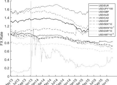
Figure 1 plots exchange rates relative to the USD during our sample time period from 1 May 2013 until 31 December 2015. Note that the XBT/USD exchange rate exhibits much higher volatility than traditional fiat currency exchange rates. The largest peak corresponds to 29 November 2013, after a surge in retailer announcements that they would soon be accepting Bitcoin as payment (see, e.g., Jopson and Foley, 2013), and after a hearing by the U.S. Senate demonstrated that they would take a

more neutral position regarding digital currencies (see, e.g., Eha, 2013).

[Insert Figure 1 about here.]

We collect fiat currency bid and ask quotes provided by the exchange rate service WM/Reuters for our sample time period. Bid and ask quotes are available for 60 out of 90 possible combinations of fiat currencies. The quotes are downloaded from Thomson Reuters Datastream, and are originally sourced from wholesale electronic currency platforms, including Thomson Reuters Matching, EBS, and Currenex, to reflect an average of interbank quotes between 3:59:30pm and 4:00:30pm GMT (10:59:30am and 11:00:30am ET). Based on theaskandbidquotes,S_t,A/B^a andS_t,A/B^b , the absolute spread is given by their difference,S_t,A/B^a −S^b_t,A/B, and the percentage spread as the absolute spread relative to the ask quote, ^S

a

t,A/B−S^b_t,A/B

S^a_t,A/B . Additionally, percentage bid-ask spreads for Bitcoin for the same time period are downloaded from Bitcoinity (data.bitcoinity.org/); the data includes percentage bid-ask spreads for all exchange rates except for against the Mexican peso (MXN) and the South African rand (ZAR).

Bid-ask spreads are provided separately for each Bitcoin exchange, so we take the median bid-ask spreads across exchanges. Bitcoinity calculates percentage bid-ask spreads as the percentage difference between the daily minimum ask quote and maximum bid quote; thus, these spreads do not represent a spread that would be available to a trader at a particular time, but represent an upper bound on bid-ask spreads in the Bitcoin market.

Table 2 presents summary statistics for percentage bid-ask spreads for the nine fiat exchange rates against the USD, as well as the eight exchange rates against Bitcoin. From the table, it is clear that Bitcoin spreads tend to be much higher than those of fiat currencies. For example, the percentage spread for trading EUR against XBT is more than 40 times larger than the spread for trading EUR against USD. Our estimates of Bitcoin spreads tend to be larger than those in the existing literature (see, e.g., Kim, 2017; Brauneis et al., 2019), for several reasons. First, most studies only consider highly liquid Bitcoin pairs, such as USD/XBT, while we additionally consider other, less liquid, pairs.

Secondly, our data only extends until 2015, so other studies using more recent data may show lower spreads as liquidity in Bitcoin markets has grown over time.

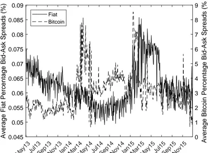
Figure 2 plots the average percentage bid-ask spreads for exchange rates involving fiat currencies only and the average percentage bid-ask spreads for Bitcoin exchange rates over our sample time period.

The plot again highlights the difference in magnitude between the two groups of spreads, and also shows that they tend to follow different dynamics. Spreads for Bitcoin begin to rise in early February 2014,

i.e., right around the Mt. Gox bankruptcy, spiking at 8.1% several weeks later on 31 March 2014.

Interestingly, both Bitcoin and fiat currency spreads peak in January-February 2015, likely a result of the Swiss National Bank’s abrupt announcement on 15 January 2015 that it would end its cap on the CHF/EUR exchange rate (see, e.g., Jolly and Irwin, 2015).

[Insert Table 2 and Figure 2 about here.]

3 The Triangular Arbitrage Parity

A consequence of no-arbitrage pricing, which is a cornerstone in modern financial theory, is that there are strong theoretical predictions concerning the relationships between the prices of financial assets. In this paper, we consider no-arbitrage prices between triplets of exchange rates. Consider three currencies A,B, and so-called “vehicle currency”V, that trade in a foreign exchange market that is absent trading constraints and costs, in which agents are perfectly informed and have no market power. In the absence of arbitrage, for any triplet of spot exchange rates S_t,A/B,S_t,A/V andS_{t,V /B}, we obtain thetriangular arbitrage parity:

S_t,A/B = S_t,A/VS_{t,V /B} or, equivalently, lnS_t,A/B = lnS_t,A/V + lnS_{t,V /B} . (1)

In a hypothetical frictionless and arbitrage-free market, we therefore should always observe lnS_t,A/B− lnS_t,A/V −lnS_{t,V /B}= 0 exactly. However, for our empirical exchange rate data described in Section 2, we observe lnS_t,A/B−lnS_t,A/V −lnS_{t,V /B}̸= 0 for all periodstand all currency triplets in our sample.

Under “normal” market conditions, small deviations from arbitrage parities are, of course, expected to persist, for example, due to transaction costs. The presence of transaction costs creates so-called “no- arbitrage bounds”, within which the cost of an arbitrage trade is larger than its profit and thus these deviations persist in the market (see, e.g., Modest and Sundaresan, 1983; Klemkosky and Lee, 1991;

Engel and Rogers, 1996). Therefore, such deviations do not necessarily constitute tradable arbitrage opportunities in practice.

Therefore, in a first step, we explore whether our observations that lnS_t,A/B−lnS_t,A/V−lnS_{t,V /B}̸=

0 can be explained by transactions costs implied by bid-ask spreads. Specifically, we investigate whether the deviations from the triangular parity stay within no-arbitrage bounds implied by transaction costs as measured using bid-ask spreads. As the difference between bid and ask prices represents the profit

earned by brokers to facilitate the market between buyers and sellers, the bid-ask spread represent a significant cost for a “round-trip” trade, and therefore the bid-ask spread is often used as a measure of transaction costs.

To calculate no-arbitrage bounds, we follow equation (6) of Kozhan and Tham (2012) and consider the following “bid-ask adjusted” no-arbitrage conditions, given 0< S_t,A/B^b ≤S_t,A/B^a :

S_t,A/B^a ≥S^b_t,A/VS_{t,V /B}^b and S_t,A/B^b ≤S_t,A/V^a S^a_{t,V /B}. (2)

Assuming that the midquote (i.e., the mean bid and ask quote) represents the true underlying value of the exchange rate, and assuming non-zero spreads, the implied cost of a transaction is equal to the half-spread, e.g., C_t,A/B := ^S

a

t,A/B−S_t,A/B^b

2 ≥ 0. Define the implied transaction costs relative to the midquote for the three currency pairs by c_t,A/B,c_t,A/V andc_{t,V /B}. Then,S^a_t,A/B=S_t,A/B+C_t,A/B= S_t,A/B(

1 +c_t,A/B)

andS_t,A/B^b =S_t,A/B−C_t,A/B =S_t,A/B(

1−c_t,A/B)

. By using these equations and the no-arbitrage conditions in (2), we obtain the no-arbitrage bounds:

(1−c_t,A/V) (

1−c_{t,V /B})

(1 +c_t,A/B) ≤ S_t,A/B S_t,A/VS_{t,V /B} ≤

(1 +c_t,A/V) (

1 +c_{t,V /B})

(1−c_t,A/B) . (3)

By taking logarithms we get:

c_t,L≤lnS_t,A/B−lnS_t,A/V −lnS_{t,V /B}≤c_t,R, (4)

where the lower boundct,L is given by ln(

1−ct,A/V

)+ ln(

1−ct,V /B

)−ln(

1 +ct,A/B

)and the upper boundct,R is given by ln(

1 +ct,A/V

)+ ln(

1 +ct,V /B

)−ln(

1−ct,A/B

).

To obtain conservative no-arbitrage bounds, we consider the minimum of the lower bound ct,L, denoted ¯cL, and the maximum of the upper bound ct,R, denoted ¯cR in the following. In addition, we obtain the 10% percentile, the mean, the median and the maximum of the lower bound (denoted cL,10%, cL,mean, cL,median and c_L), and the minimum, the mean, the median and the 90% percentile of the upper bound (denoted c_R, cR,mean, cR,median and cR,90%). Since the Bitcoin bid-ask spreads are obtained from various exchanges and include some extreme realizations, the 10%/90% percentile measures are calculated in order to exclude possible effects arising from such spikes in the bid-ask spread.

Table 3 presents relative frequencies at which the deviations of lnS −lnS −lnS

from zero exceed our bid-ask spread-implied measures of no-arbitrage bounds. For all fiat currency triplets, we find that the deviations stay well within the no-arbitrage bounds implied by bid-ask spreads.

Interestingly the deviations remain within the interval [c_L, c_R]. One caveat to this result might be the different time windows use for the calculation of spot rates (12pm ET) and bid and ask quotes (4pm GMT/11am ET). Studies such as Marsh et al. (2017) and Evans (2018) have focused on the fact that fiat currency markets display vastly different market microstructure dynamics during the “4pm London Fix”, as large banks flood the market with liquidity in attempts to influence this benchmark spot rate.

However, these studies show that spreads during the 4pm GMT window are muchlower than at other times during the trading day. This would therefore bias our results towards finding more deviations outside the bounds.

On the other hand, Bitcoin currency triplets are shown to exceed the no-arbitrage bounds much more often. Whenever the currency Bitcoin is included a modest proportion of the deviations lnS_t,A/B− lnS_t,A/V −lnS_{t,V /B} does not meet the conservative no-arbitrage bounds described by ¯c_Land ¯c_R. This is particularly striking, considering that the maximum spread measure is much higher for Bitcoin (see Table 2). By using the percentile based no-arbitrage bounds we observe that a substantial proportion of the deviations is outside the interval [c_L,10%, c_R,90%].

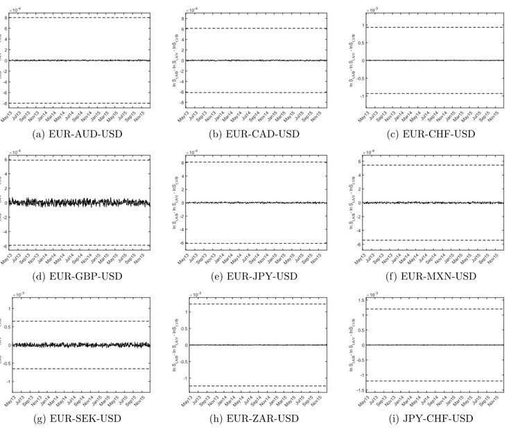
The tendency of fiat currency non-zero deviations of lnSt,A/B−lnSt,A/V−lnSt,V /Bto stay within no- arbitrage bounds can also be seen by plotting these deviations over time. Figure 3 presents deviations, along with the no-arbitrage bounds implied by the 10%/90% percentiles of spreads, for a representative sample of currency triplets including only fiat currencies, in which the U.S. dollar is used as the vehicle currency. Deviations for fiat currency triplets in which the euro is used as the vehicle currency look very similar. These deviations are quite small in magnitude, remaining in the interval [−0.0001,0.0001] or even smaller, and are fluctuating around zero with no clear episodes of being positive or negative only.

Emphasizing the results from Table 3, the deviations remain far way from the no-arbitrage bounds.

This holds even for currencies such as the Mexican peso and South African rand, which likely have higher transactions costs due to their relatively low trading volumes.

[Insert Figure 3 about here.]

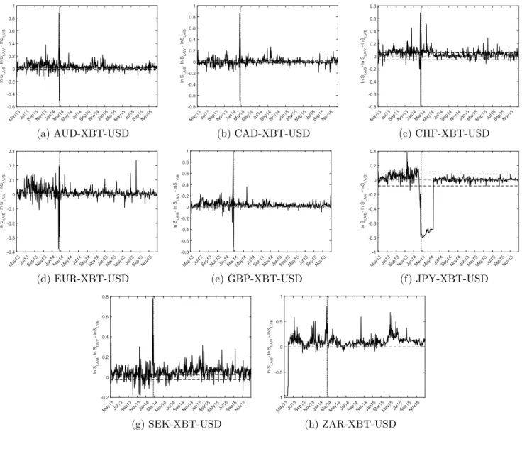
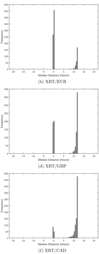
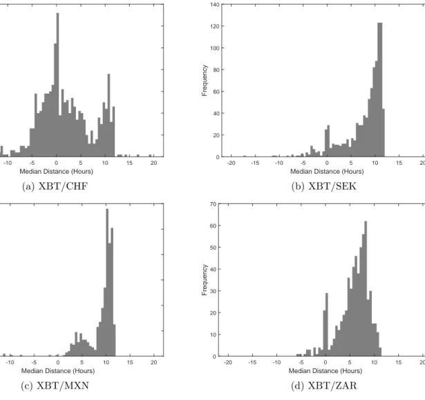
For comparison, Figure 4 presents all deviations for triplets including Bitcoin, in which USD is used as the vehicle currency, along with our measures of no-arbitrage bounds implied by the 90% percentiles of spreads. It is clear that including Bitcoin into the currency triplets leads to both higher magnitudes

and higher volatility of the deviations. These deviations are often shown to exceed the no-arbitrage bounds. Furthermore, we observe time spans in which the deviations remain systematically positive or negative, pointing to persistent over- and underpricing in the market for Bitcoin. Such mispricings may persist, for example, due to the relatively low rate of informed institutional trading on Bitcoin exchanges.

Anecdotal evidence puts the amount of Bitcoin held by institutional investors at about 1% as of 2017 (see, e.g., Lielacher, 2017). Furthermore, the most recent data from the Bitcoin trading services provider itBitshows that institutional investors make up a majority of OTC Bitcoin transactions, implying that when they do trade, they may prefer to do so off-exchange (see Hamilton, 2016). Interestingly, most Bitcoin triplets experience a spike in their deviations around the Mt. Gox bankruptcy on 24 February 2014 (marked by the blue dotted line in the plots), showing the impact that this event had on the market for Bitcoin. By contrast, for fiat currency triplets we do not observe spikes around this date.

Therefore, it may be that profitable arbitrage opportunities exist in the market for Bitcoin. However, it may also be that there are additional trading costs or frictions for Bitcoin that are not captured by bid- ask spreads, which limit the profitability of correcting deviations from the triangular arbitrage parity.

Such trading costs may come, for example, from high exchange fees; Kim (2017) estimates a maximum Bitcoin exchange fee of about 0.5%, while Fink and Johann (2014) document Bitcoin exchange fees up to 2%. Another factor is the high latency of Bitcoin trading; Courtois et al. (2014) show that Bitcoin transactions can take up to ten minutes, making it difficult to engage in simultaneous transactions with lower latency fiat currency markets. Bitcoin traders can opt for more speed, but this requites the payment of a so-called “mining fee”, which Fink and Johann (2014) estimate as about 1%-4% for Bitcoin. There are also a number of additional risks that are relatively unique to Bitcoin – such as higher risks of exchange insolvency and theft (see, e.g., Moore and Christin, 2013), or its association with illegal activity (see, e.g., Foley et al., 2019).

After examining deviations from the log-form of the triangular arbitrage parity, i.e., of lnSt,A/B− lnSt,A/V −lnSt,V /B from zero, and a brief comparison of these deviations to the no-arbitrage bounds implied by bid-ask spreads, the next section will analyze whether these deviations are connected to sig- nificant market dislocations, in terms of deviations from a stochastic version of the triangular arbitrage parity with cointegrated exchange rates and stationary errors and with parameter values as implied by the exact parity.

4 Monitoring Market Dislocations

In this section we discuss the logarithmic form of the triangular arbitrage parity from a cointegration perspective, as a basis to identify market dislocations as breakdowns of the prevalence of a cointegrating relationship with parity-implied values of the parameters. To be precise, we consider:

lnS_t,A/B = µ+β^⊤

⎛

⎝

lnS_t,A/V lnS_{t,V /B}

⎞

⎠+u_t,

yt = µ+β^⊤xt+ut, (5)

in which the three involved exchange rates S_t,A/B, S_t,A/V andS_{t,V /B} are integrated and the errorsu_t stationary. The I(1) properties of the exchange rates are discussed and confirmed in Appendix A.1.

The triangular arbitrage parity implies thatµ = 0 and β = (1, 1)^⊤. With the parameter values implied by the parity, the unobserved errorsu_tbecome in fact observed quantities. The idea of the mon- itoring procedure of Wagner and Wied (2015) and Wagner and Wied (2017) is to assess the stochastic properties of the residuals ˆu_t,m, defined as:

ˆ

ut,m=yt−µˆm−(1, 1)xt, t= [mT] + 1, . . . , T, (6)

with ˆµm:= _[mT]¹ ∑[mT]

t=1 (yt−(1, 1)xt), the OLS estimate of µfor the given value ofβ= (1, 1)^⊤ over thecalibrationperiod 1, . . . ,[mT] for some 0< m <1. The calibration periodt= 1, . . . ,[mT] is known to be or assumed to be free of structural breaks. Note that we estimate the intercept µrather than setting it equal to µ= 0, as implied by the triangular arbitrage parity. This is to allow for rounding errors, as the convention of quoting exchange rates at only four decimals places (two decimal places in the case of the yen) typically leads to small non-zero means in (6). Note also that the variant of the monitoring procedure we use is treated in full detail only in Wagner and Wied (2015), since we monitor a cointegrating relationship with known, i.e., given from the arbitrage parity condition, parameters rather than estimated parameters.

As long as the relationship in (5) continues to hold after the calibration period, the residuals ˆutwill continue to be stationary. Should the relationship break down, however, either because the parameters change (away from the parity-implied values) or because cointegration breaks down altogether, the residuals will become “big”. This suggest to consider, e.g., a stationarity test statistic as the basis for a

monitoring statistic. Wagner and Wied (2017) consider as starting point the Kwiatkowski et al. (1992) test statistic, which is transformed into a monitoring statistic given by:

Hˆ^m(s) := 1 ˆω²_m

1 T

[sT]

∑

j=[mT]

( 1

√ T

j

∑

t=1

ˆ ut,m

)²

, (7)

withm≤s≤1 andωˆ_m² is an estimator of the long-run variance ofu_t, i.e., of 0< ω²=∑∞

j=−∞Eu_t−ju_t<

∞, calculated over the calibration period 1, . . . ,[mT]. In our application we estimateω²non-parametrically, using the Bartlett kernel and the bandwidth rule of Andrews (1991). The test statistic has to be nor- malized by the long-run variance to take into account potential serial correlation inu_t. Under the null hypothesis of no structural change, it holds that:

Hˆ^m(s)⇒H^m(s) := 1 ω²

∫ s m

ω²W˜(r)²dr=

∫ s m

˜W(r)²dr , (8)

with ˜W(r) =W(r)−_m^rW(m) andW(r) standard Brownian motion. The monitoring statisticHˆ^m(s) is calculated for all [mT] + 1≤[sT]≤T and a weighted version of it is compared with critical values obtained from Wagner and Wied (2015). A structural break is identified when a weighted test statistic,

Hˆ^s(m)

g(s) , exceeds, in absolute value, the corresponding critical value, i.e.:

τ_m:=

{

min

s: [mT]+1≤[sT]≤T

⏐

⏐

⏐

⏐

⏐ Hˆ^m(s)

g(s)

⏐

⏐

⏐

⏐

⏐

> c(α, g(s), m) }

, (9)

where τm, referred to as the detection time, is a natural estimator of the break-point. In our case we use the weighting function g(s) = s³ as in Wagner and Wied (2017). The critical values c(α, g(s), m) depend upon the significance levelα, the weighting functiong(s) and the length of the calibration period

m. They are constructed such that P

(

sup_m≤s≤1

⏐

⏐

⏐

⏐

∫s mW˜(r)²dr

g(s)

⏐

⏐

⏐

⏐

> c(α, g(s), m) )

=α. Throughout our

empirical analysis we use a significance level ofα= 5%. The functioning of the monitoring procedure is illustrated in Figure 5, with a break-point detected at time pointtτ_m := [τmT].

[Insert Figure 5 about here.]

Looking at (6) is informative for understanding why the monitoring procedure has power against both a change in the stochastic behavior of the errors as well as against changes in the parameters oc- curring in the monitoring period. Consider for brevity the omnibus case thatpotentially all parameters

change at some time point [rT], with the new parameters from [rT] + 1 onward equal toµ₁̸=µ₀, with µ₀ the true value in the calibration period, andβ₁̸= (1, 1)^⊤. This implies that, for the residuals, the partial sum process:

√1 T

T

∑

t=[rT]+1

ˆ

u_t= 1

√T

T

∑

t=[rT]+1

u_t−T−[rT]

√T (ˆµ_m−µ₁)− 1

√T

T

∑

t=[rT]+1

((1, 1)−β^⊤₁)x_t (10)

will diverge. In case ut changes its behavior from I(0) to I(1) or to an explosive process, the partial sum process ^√1

T

∑T

t=[rT]+1utdiverges, and in case the intercept changes toµ1, the corresponding term will diverge as ˆµm−µ1 will in this case not converge to zero due to ˆµm converging to the true value prior to the change, µ0. The same argument applies if the slope parameter vectorβ changes, since in that case ((1, 1)−β₁^⊤) is not equal to zero and the corresponding term involvingxtdiverges. Thus, in either case of structural change, the partial sum process ^√1

T

∑T

t=[rT]+1uˆt, which converges under the null hypothesis, will diverge, being either an integrated or explosive process or including a deterministic trend or both.

Of course, the first step in assessing whether the posited parity relationship in (5) is supported by the data is to estimate the parameters µandβ and to verify whether the estimated parameters are in line with the no-arbitrage valuesµ= 0 andβ= (1, 1)^⊤. When estimating the parameters in (5) one has to resort to estimators that have limiting distributions that allow for asymptotic standard inference. These estimators correct for the effects of error serial correlation and regressor endogeneity that contaminate the limiting distribution of the OLS estimator. In our analysis, we use the so-called fully modified OLS (FM-OLS) estimator of Phillips and Hansen (1990). In particular, we performrolling estimation of the parameters with FM-OLS to assess the stability of the parameters visually in the following Section 5.

A detailed discussion of modified least squares estimators in cointegrating regressions is contained, e.g., in Wagner (2018). Since the limiting distribution of the FM-OLS estimator allows for asymptotically valid inference, we also use the FM-OLS estimates over the full sample period to test several hypotheses related to whether the parameters are equal to the parity-implied values. This is, of course, nothing but an additional way to assess whether the parameters are close to the parity-implied values. Neither of these tools, however, allows for asymptotically valued detection of break-points, the reason being that monitoring is inherently a multiple testing problem and this has to be taken into account in the construction of a valid monitoring procedure, not least in the construction or simulation of valid critical values that allow for asymptotic size control. See Chu et al. (1996) for a detailed discussion of these

issues.

5 Results

This section describes the results from our empirical investigation of the triangular arbitrage parity in the foreign exchange and Bitcoin markets. Recall that the triangular arbitrage parity examines the relationship between a triplet of exchange rates. Like Pasquariello (2014) we include only currency triplets in which either USD or EUR serve as vehicle currency. Furthermore, each currency triplet is only included once, irrespective of the ordering. This leaves us with 72 fiat currency triplets and 18 currency triplets involving Bitcoin. Furthermore, we choose a calibration period of m= 0.2. As our sample period ranges from 1 May 2013 until 31 December 2015, this means that our calibration time period lasts from 1 May 2013 until 8 November 2013, which corresponds to a relatively stable period for exchange rates.

First, we want to see whether estimates of the parametersµandβfrom (5) correspond to the values implied by the triangular arbitrage parity, µ= 0 andβ = (1, 1)^⊤. We estimate the parameters over the full period, 1 May 2013 to 31 December 2015, using fully modified least squares (FM-OLS), which corrects for possible serial correlation as well as endogeneity in a cointegration regression (see Phillips and Hansen, 1990). We subsequently analyze Wald-type tests to separately test the parameters for µ= 0,β₁= 1, and β₂= 1. The results for these Wald tests are presented in Table 4.

[Insert Table 4 about here.]

We are much more likely to find deviations fromµ= 0 in the currency triplets that include Bitcoin, For the USD triplets, the Wald-type test rejects (at a 5% confidence level) the null hypothesis that µ = 0 for only 4 out of 36 (11%) of the fiat-only currency triplets, but for 7 of the 9 (77%) of the currency triplets that include Bitcoin. Similarly, for the EUR triplets, we reject the hypothesis that µ= 0 in only one (2.7%) of the fiat-only triplets, and in seven of the Bitcoin triplets. Meanwhile, we are also more likely to find deviations fromβ= (1, 1)^⊤ in Bitcoin triplets, though there are overall fewer deviations than for µ. Combining both the USD and EUR triplets, we reject the hypothesis β₁ = 1 only twice (2.7%) out of the possible 72 fiat-only triplets, and in 6 (33%) of the Bitcoin triplets. The hypothesis β₂ = 1 is never rejected for the fiat-only triplets and is reject for 4 (22%) of the Bitcoin triplets. Therefore, in all cases, we are more likely to see deviations from the parity-implied parameter

values for currency triplets that include Bitcoin.

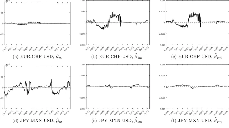
Next, we examine the stability of the parameter estimates over time, using rolling window regressions to visually inspect whether the parameter estimates are close to the values implied by the triangular arbitrage parity. We consider rolling window parameter estimates for the regression model (5), using a window size m = 0.2 as a proportion of the total time series length, and abbreviate the estimated parameters byµˆ_m andβˆ_m=(

βˆ_1m,βˆ_2m)^⊤ .

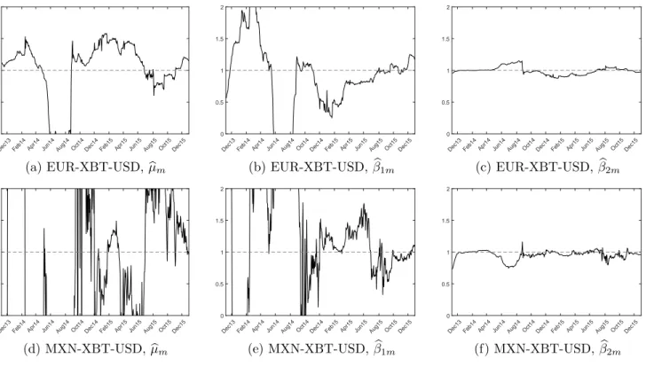
Representative results for the estimatesµˆ_mandβˆ_mare provided in Figures 6 and 7. Figure 6 shows rolling window estimates for currency triplets in which only fiat currencies are included, and reveals that the estimated parameters hardly deviate from their theory-implied values over our sample period, and that the variation of the estimates is small. On the other hand, the rolling window estimates for currency triplets involving Bitcoin, shown in Figure 7, show high variation in the estimates and large deviations away from the theory-implied parameter values.

[Insert Figures 6 and 7 about here.]

In a next step, we perform stationarity monitoring as described in Section 4, which will also allow us to identify dates around which structural breaks-points are more likely to have occurred. Overall, given the frequent observation of deviations outside of no-arbitrage bounds for currency triplets involving Bitcoin (see Figure 4), as well as deviations of parameter estimates away from their theory-implied values from the rolling window regressions (see Figures 6 and 7), we might expect that our monitoring tool will be more likely to reject the null hypothesis of “no structural breaks” in the cointegrating relationship for Bitcoin currency triplets. In our stationary monitoring procedure, we fix β =β^∗ = (1,1)^⊤ and monitor the OLS residualsˆu_t:=y_t−µˆ_m−β^{∗ ⊤}x_t. The detected break-points are presented in Table 5.

[Insert Table 5 about here.]

The results indeed indicate that we are much more likely to detect a break-point in the triplets that include Bitcoin. With the USD as the vehicle currency, we observe six break-points in the triplets that include Bitcoin (XBT) (i.e., in two-thirds of the Bitcoin triplets), and only two break-points when the triplet is composed of fiat currencies only (5.5% of the fiat-only triplets). Interestingly, the two breaks in the fiat-only triplets both include the Mexican peso (MXN), with break-point dates in October 2014. The Mexican peso experienced a rapid decline at the end of 2014 due to a drop in oil prices and strengthening of the U.S. dollar, which might have generated these deviations (see, e.g., Bain, 2013).

Similarly, using the EUR as the vehicle currency leads to seven break-points in the Bitcoin triplets, and to zero breaks in the fiat-only triplets.

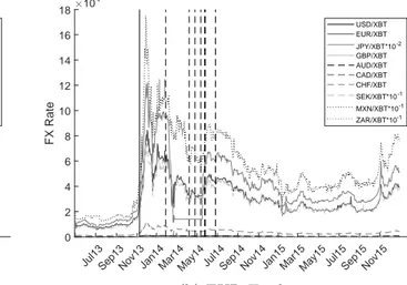
As we have shown that a high number of break-points are detected in the Bitcoin triplets, the next question is whether the detected break-points tend to be clustered in time. Figure 8 plots the Bitcoin exchange rates, with dashed vertical lines representing the detected break-points for currency triplets using either the USD or EUR as vehicle currencies. The detected break-point of 26 February 2014 for the triplet JPY-XBT-USD comes just days after the Mt. Gox bankruptcy. That the bankruptcy should hit the market for JPY/XBT the hardest is no surprise; the shut-down of the Tokyo-based exchange represented a massive disruption to the market for Bitcoin against the yen, as Bitcoin dropped 17.41%

against the yen within a single day. Furthermore, as Mt. Gox is the only exchange in our dataset that offered JPY/XBT transactions at the time, its bankruptcy meant a virtual halt on exchange-based trading of yen for Bitcoin. However, it’s important to note that there may have been more exchanges offering JPY/XBT that have chosen not to self-report in the bitcoincharts dataset, and furthermore that traders could search for counterparties in JPY/XBT via OTC markets.

[Insert Figure 8 about here.]

Other break-points for USD triplets do not seem to be clustered in time, although all take place after the Mt. Gox bankruptcy. It is not clear whether these later detection dates are due to a lagged reaction of our detector, or reactions to other market events. For example, it is likely that the break-point of 19 January 2015 for the triplet CHF-XBT-USD is a result of the Swiss National Bank’s abrupt ending to its cap on the CHF/EUR exchange rate just a few days earlier.

For the triplets using EUR as a vehicle currency, depicted in Figure 8b, interestingly we see that the break-points indeed tend to be clustered in time, with most break-points clustered around the bankruptcy of Mt. Gox and the subsequent recovery. The only exception is JPY-XBT-EUR; for this triplet, we already detect a break-point on 29 January 2014, before the Mt. Gox bankruptcy. Mt.

Gox was experiencing problems throughout early 2014 in the lead-up to its bankruptcy, as customers complained about withdrawal delays and poor service (see, e.g., Weisenthal, 2014). Meanwhile, the break-points for almost all remaining Bitcoin triplets occur during the weeks and months after the Mt.

Gox bankruptcy, when trading was likely much more restricted due to the collapse of the major ex- change. Our results imply that these trading restrictions may have led to deviations from the triangular arbitrage parity for Bitcoin traders in a variety of currencies. However, given difficulties in trading, it is

possible that Bitcoin traders were not able to take advantage of these potential arbitrage opportunities.

Figure 9 plots the OLS residualsuˆ_t:=y_t−ˆµ_m−β^{∗ ⊤}x_tas described in Section 4, for two examples of triplets: one in which a break-point is detected (JPY-XBT-USD, Figure 9a), and one in which no break-point is detected (JPY-SEK-USD, Figure 9b). In the figures, the solid lines correspond to the cut-off between the calibration and monitoring time periods, and the dashed lines correspond to the detected break-point (if any) for the currency triplet shown. In Figure 9a, the break-point of 26 February 2014 corresponds to a downward spike in the residuals; furthermore, after the detected break- point, the residuals remain consistently negative. For comparison, Figure 9b shows a triplet for which no break-point is found. These residuals remain clustered around zero.

[Insert Figure 9 about here.]

Note that break-point detected by means of our monitoring tool does not automatically imply that exploitable arbitrage opportunities exist. The deviations from triangular arbitrage could be due to costs and trading constraints that would prevent a profitable trade based on the deviations. For example, as mentioned above, small deviations in µ from zero can be justified by rounding errors or measurement effects. However, a break-point detected by our monitoring tool implies a break down in the cointegrating relationship between exchange rates, and thus indicates a substantial dislocation between the markets for these currencies.

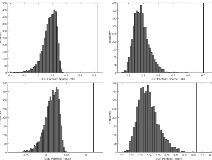
5.1 Portfolio Trading Strategy

In a final step, we check whether our results could be used to construct a profitable trading strategy. The idea is to compare two portfolios: one based on a simple buy-and-hold strategy, and one that trades once a break in triangular arbitrage parity deviations is detected according to the Wagner and Wied (2017) monitoring procedure. If detected break-points indeed represent market dislocations, then a break may signal higher expected uncertainty in currency markets. Thus, it may be profitable to re-balance the portfolio away from the implicated currencies and back into their domestic currency. This strategy is similar to those explored in Wied et al. (2012) and Wied et al. (2013), and is furthermore similar to the portfolio re-balancing channel of Hau and Rey (2006), in which investors shift their portfolios away from foreign currencies and into their domestic currency when their exposure to exchange rate risk increases. We consider either USD or EUR as the domestic currency. Furthermore, the initial and liquidation dates for both portfolios are defined as the first and last dates of the monitoring period in

our sample, such that the total duration of both portfolios is from 11 November 2013 until 31 December 2015, i.e., t = [mT] + 1, ..., T. We further assume that any trade can be executed at the noon spot exchange rates described in Section 2.

The first portfolio (denoted by Portfolio A) consists of a simple buy-and-hold strategy that divides 100 units of the domestic currency equally between the eleven currencies in our sample (USD, EUR, JPY, GDP, AUD, CAD, CHF, SEK, MXN, ZAR, and XBT), and never trades the currencies after the initial purchase. We assume that currencies are deposited and earn the local risk-free rate, taken as the local one-month deposit rate, as collected from Thomson Reuters Datastream and transformed to a daily interest rate such that daily returns can be compounded. As there is no risk-free Bitcoin- denominated asset, we assume that the risk-free rate for Bitcoin is zero. We assume that the units of foreign currency are exchanged for the domestic currency only on the liquidation date, leading to buy-and-hold return R^A, which denotes the return of Portfolio A over the entire portfolio duration.

Note that changes in the value of the buy-and-hold portfolio are, in addition to compound interest, driven by currency revaluations over the portfolio duration. Hence, Portfolio A captures the mean performance of a domestic currency against the other ten currencies considered, after accounting for compound interest.

The second portfolio (denoted by Portfolio B) similarly divides 100 units of the domestic currency equally between the eleven currencies, but trades on the day(s) on which our monitoring procedure detects any break-point in the triangular arbitrage parity deviations. Specifically, it exchanges those holdings in the foreign currencies involved in the triangular arbitrage triplet implicated by the break- point to the domestic currency. For example, let USD be the domestic currency. From Table 5, the first breakpoint is experienced by the triplet JPY-XBT-EUR on dateτ1=29 January 2014. On this date, the spot rates were Sτ₁,U SD/J P Y = 0.0098, Sτ₁,U SD/XBT = 834.9783 and Sτ₁,EU R/U SD = 0.7320. Given the yen-denominated risk-free rate, the initial units of 905.8119 JPY will be worth 905.9270 JPY by time τm,1. The trading strategy will then exchange the 905.9270 units of JPY for 905.9270×Sτ₁,U SD/J P Y = 8.8659 units of USD. The strategy will also convert the units of XBT and EUR into units of USD.

For all subsequent breaks, if one of the implicated foreign currencies was already involved in any prior break, the investor already converted the corresponding holdings into the domestic currency and so does not trade in that currency. Finally, at the liquidation date, all remaining foreign currency holdings are converted to the domestic currency. A summary of the dates on which Portfolios B trades can be found in Table 6, for both the USD and EUR as the domestic currency. The return earned by Portfolio