Variational search for control pulses suppressing decoherence

Variational search for control pulses suppressing decoherence

Masterarbeit

zur Erlangung des akademischen Grades Master of Science

vorgelegt von Daniel Spannenkrebs

geboren in Witten

Lehrstuhl für Theoretische Physik I Fakultät Physik

Technische Universität Dortmund

2014

Contents

1 Introduction and Motivation 1

1.1 Model . . . . 4

1.1.1 Semiclassical central spin model . . . . 4

1.1.2 Noise model . . . . 6

1.2 Supression of decoherence . . . . 8

1.2.1 Time evolution operator . . . . 9

1.2.2 Frobenius norm . . . . 13

1.2.3 Conditions for amplitude-modulated pulses . . . . 15

1.2.4 Conditions for frequency-modulated pulses . . . . 17

2 Variational Calculation for Amplitude-Modulated Pulses 18 2.1 Variational ansatz . . . . 18

2.1.1 Functional . . . . 20

2.1.2 Lagrangian . . . . 20

2.1.3 Euler-Lagrange equation . . . . 22

2.2 Analytical solutions . . . . 28

2.2.1 General solution function . . . . 28

2.2.2 Solutions under the auxiliary conditions . . . . 29

2.3 Numerical solutions . . . . 33

2.3.1 Scheme of the programs . . . . 33

2.3.2 Symmetrical solutions . . . . 35

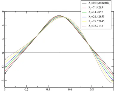
2.3.3 Asymmetrical solutions . . . . 40

2.3.4 Discussion . . . . 42

3 Simulation of the Pulses 43 3.1 Scheme of the program . . . . 44

3.2 Results . . . . 44

3.3 Discussion . . . . 48

4 Variational Ansatz for Frequency-Modulated Pulses 48 4.1 Minimized functions . . . . 49

4.2 Lagrangian . . . . 50

4.3 Euler-Lagrange equation . . . . 51

4.4 Discussion . . . . 57

5 Conclusion and outlook 58

A Analytical solutions 61

B Pseudocode 62

C Simulation Fits 62

Abstract

Suppression of decoherence is a necessary prerequisite for quantum computation and NMR spectroscopy. In these areas of research control pulses play an important role because they are used to perform necessary operations. The influence of a pulse on decoherence can be investigated via the central spin model. An important task is the search for pulse shapes which suppress the decoherence effectively.

This work addresses the search for decoherence suppressing pulses. To describe the

physical situation a semiclassical form of the central spin model with a cusp-like au-

tocorrelation is used. We introduce a variational search method which leads after an-

alytical calculations to an Euler-Lagrange equation. For amplitude-modulated pulses

analytical and numerical methods to find solutions of the Euler-Lagrange equation are

presented. The pulse which we assume to be the most important outcome of these

methods in terms of decoherence suppression is tested via a simulation program writ-

ten by Stanek. In addition the variational method is applied to frequency-modulated

pulses but the Euler-Lagrange equation is not solved within this work.

Zusammenfassung

Dekohärenzunterdrückung ist eine notwendige Voraussetzung für Quanten- informationsverarbeitung und NMR-Spektroskopie. In diesen Forschungs- bereichen spielen Kontrollpulse eine wichtige Rolle weil sie für notwendige Op- erationen verwendet werden. Der Einfluss eines Pulses auf die Dekohärenz kann im Zentralspinmodell untersucht werden.

Diese Arbeit beschäftigt sich mit der Suche nach dekohärenzunterdrückenden Pulsen. Um die physikalische Situation zu beschreiben, wird eine semiklassis- che Form des Zentralspinmodelles mit einer spitzen Autokorrelation verwendet.

Wir stellen eine Variationsrechnung als Suchmethode vor, die nach analytis-

chen Rechnungen zu einer Euler-Lagrange Gleichung führt. Für amplituden-

modulierte Pulse werden analytische und numerische Methoden vorgestellt, um

die Lösungen zu finden. Der Puls, den wir für das wichtigste Ergebnis dieser

Methoden bezüglich der Dekohärenzunterdrückung halten, wird mit einem von

Stanek geschriebenen Simulationsprogramm getestet. Als Ergänzung wird die

Variationsmethode auch auf frequenzmodulierte Pulse angewendet, aber die

Euler-Lagrange Gleichung wird in dieser Arbeit nicht gelöst.

1 Introduction and Motivation

Control pulses are a fundamental part of quantum computation and NMR spectroscopy.

An important tool to of the theoretical description of these topics is the central spin model in all of its different versions. Typical examples of these versions are the quantum mechan- ical central spin model and the semiclassical central spin model.

Since the realization of devices using quantum information processing seems to be a pos- sible task in the foreseeable future, the central spin model has undergone an intensive development. The idea of storing information in quantum systems exists principally al- most since the beginning of quantum mechanics [1] but significant investigations aiming into the direction of devices based on quantum information processing started mainly in 1982. In that year Benioff did some considerations about the simulation of a classical sys- tem by a quantum system [2] and Feynman did some considerations on the opposite case, namely the simulation of a quantum system by a classical system [3]. The application of pulses in NMR spectroscopy is used since 1949, three years after the development of NMR spectroscopy [4].

Quantum information processing in comparison with classical information processing has besides other advantages the main advantage of the so called quantum parallelism [1]. It is the potential of a quantum computer to perform multiple operations at the same time whereas a classical computer has to perform the same operations one after another. This is not an advantage from which a quantum computer benefits in every case. This advantage can be used just for suitable problems and the algorithms have to be written in such a way that they make use of this advantage. But if these conditions are fulfilled, the advantage can be huge in comparison with a classical computer. There are several examples for al- gorithms written for quantum computers.

A famous example for a quantum algorithm is the Shor algorithm [5] which factorizes a number in polynomial time, that means, the run time depends polynomial on the bit length log(N ) of the input number N . The Shor algorithm is not just a test algorithm for quantum computers but rather a good example for an algorithm which could be really used for practical purposes. Data cryptography is based on factorization [1] and hence the Shor algorithm or similar quantum algorithms could become very useful in the field of cryptography, if an efficient quantum computer will be build.

In general every quantum system with two different energy values can be used as a quan- tum bit [1]. Possible realizations are electrons in a magnetic field captured in electron traps or quantum dots. The requirements that a physical system as a candidate for a quantum computer has to fulfill are summarized under the five DiVincenzo criteria [6].

One of these criteria is the necessity of low decoherence times of the quantum bits. The

ground steps of a quantum algorithms are operations depending on the states of one or

two quantum bits, so called quantum gates. Decoherence causes errors, that means, devia-

tion in the ground steps from the predicted operations. For a working quantum computer

a total avoidance of errors is not necessary. Instead it is enough to hold the errors per

quantum gate under a certain threshold according to the quantum threshold theorem [7].

The relevance of the central spin model for the field of quantum information processing lies in the understanding of the decoherence of a quantum bit. Decoherence is caused by different interactions of the central spin with its environment especially by the hyperfine interaction of the central spin with the nuclei in its surrounding material [8]. The relation of the central spin model to the decoherence lies in the fact that you can understand the central spin as a quantum bit and the bath spins as the disturbing environment, i.e. the nuclei in the surrounding material.

In this work we use the semiclassical form of the central spin model. This means we treat just the central spin quantum mechanically and we use an averaged classical fluc- tuating field for the bath. This does not consider the quantum mechanical effects in the bath and is hence further afar from the reality than a quantum mechanical central spin model, but the advantage is, that the semiclassical central spin model has a much easier mathematical representation and makes computational approaches much faster, because it reduces the states of a big number of bath spins to a single variable. The averaged field is known under the title Overhauser field and it is already attested that it is a justified simplification of the bath [9, 10].

The situation which we want to investigate in this work is the decoherence under ex- tern pulses with the aim to find pulse shapes which suppress the decoherence. This is interesting because in a quantum computer you have to perform operations on the qubits.

These operations have to turn the direction of the spin in the Bloch sphere by an angular of π, ^π ₂ and ^π ₄ for the Hadamard gate. These operations are a necessity because they represent the ground steps of every quantum algorithm [1, 21]. Hence control pulses are a fundamental part of quantum computation and it is vital to suppress decoherence during the application of a pulse as effectively as possible. A typical idea for quantum computers is to implement these operations via magnetic pulses.

Further relevance of control pulses lies in the fact that pulses are used in sequences for the suppression of decoherence. This is known under the title dynamical decoupling and was initiated by the discovery of the Hahn Echo, which was demonstrated in 1950 [12]. Dy- namical decoupling is investigated for sequences of equidistant and non-equidistant pulses [13]. Examples are the Carr-Purcell-Meiboom-Gill sequence [14] with preparatory work from [15] and the Uhrig-dynamical-decoupling sequence [16, 17, 18, 19].

The investigations in this work which are new within the research field of the semiclassi-

cal central spin model are mainly two points. The first one is that we use a variational

approach for the pulse search. To our knowledge the method which we use is new in this

research area. A variational approach to the topic of decoherence was already done by

conditions which we want to fulfill. Hence we treat a typical optimization problem.

The second investigation in this work lies in the noise model which we use. Previous works mainly used a Gauß distribution for the autocorrelation of the noise while we use a cusp.

This is not the first work that investigates a cusp as the autocorrelation, see for example [21] which is the most important forerunner of this work. But this noise model is much less investigated than a Gauß distribution and further research is necessary. A special feature of the cusp-like autocorrelation is a term in the expansion of the Frobenius norm that does not exist under a Gauß distribution as autocorrelation. This term was just in [21] discovered and this work continues the investigation.

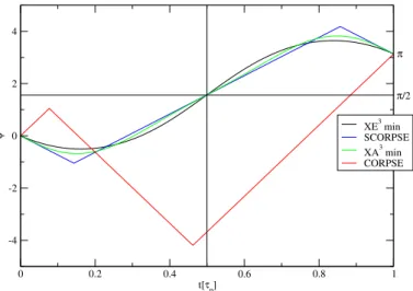
A further noteworthy aspect of this work is that we search for pulses which minimize the docoherence under an assumed energy limitation which can be caused for example by device-limits or a certain energy value that you do not want to exceed because of a limited energy supply. The forerunner of this work [21] presents the pulses under two aspects, namely an upper limit of the amplitude and a lower limit of the pulse duration. Such a limitation is a typical aspect of the search for new pulses because without any limitation it would be no problem to create a perfectly decoherence suppressing pulse and in practice you have limitations in every case. The reasons for our choice of a limited energy are rather conceptional reasons concerning the practicability of the variational approach than reasons concerning physical questions which we ask, but an energy limitation is still interesting in terms of physical questions. To show the quality of the pulses that we find within this work we show all the features of the new pulses in comparison with the already known pulses CORPSE and SCORPSE [22, 23] while SCORPSE is also called UPi in [24].

This work is structured as follows. In this chapter we give at first in chapter 1.1 an overview of the model including the semiclassical central spin model and the cusp-like noise model. Then in chapter 1.2 we present all the mathematics that we need for the pulse search.

Chapter 2 is the main part of this work where the variational calculation for amplitude- modulated pulses is presented. In chapter 2.1 we apply the ansatz to the problem and we do the first calculations which lead to an Euler-Lagrange equation. The next two chapters 2.2 and 2.3 contain the solutions of the Euler-Lagrange equation. In chapter 2.2 we present analytical solutions of a simplified form of the Euler-Lagrange equation and in chapter 2.3 we present numerical solutions of the general form of the Euler-Lagrange equation.

Chapter 3 contains a test of the best solution to verify it. The test is done by simulating the time evolution of a spin under the new discovered pulse with a program written in the forerunner work [21] which is described in chapter 3.1. In chapter 3.2 we present the results of the test and in chapter 3.3 we discuss these results.

Chapter 4 is an additional part where we apply an analogue variational approach to fre-

quency modulated pulses but we follow this approach just until we get a raw form of an

Euler-Lagrange equation because as you can see in chapter 4 problems arise which make

the calculations much more difficult than for amplitude-modulated pulses. In chapter 4.1

we explain the aims of the approach. Further we present the Lagrangian in chapter 4.2 and

the Euler-Lagrange equation in chapter 4.3 and in chapter 4.4 we discuss the situation.

Chapter 5 is the conclusion and the outlook of this work where we discuss the results within the research field of the central spin model.

1.1 Model

The model that is used in this work is the semiclassical form of the central spin model, which is presented in chapter 1.1.1. Because the semiclassical model contains a field which fluctuates statistically obeying an specific autocorrelation it is necessary to make a choise for the autocorrelation which is done in chapter 1.1.2. The formulas are from [25, 21].

1.1.1 Semiclassical central spin model

According to [25, 21] the central spin model consists of a central spin and a bath of spins arranged around the central spin. The central spin can be created by applying a static magnetic field to a spin- ¹ ₂ particle, for example an electron, so that the particle has two different energy eigenvalues in the magnetic field due to the Zeeman interaction. Without loss of generality the magnetic field and hence the axis of precession is arranged along the z-direction of the coordinate system. The contributing interactions are the interaction between the central spin and the bath spins and the interactions between the bath spins among each other.

In addition in order to do operations on the central spin an applied high-frequency pulse is included into the system and causes an interaction with the central spin. The pulse turns the direction of the spin by a predefined angular where we treat just π-pulses. The interaction between the bath spins and the pulse is neglected in this work.

In general there is also a contribution to the Hamiltonian of the static magnetic field, but to simplify the Hamiltonian the rotating wave approximation is used [25] so that this contribution is not noticeable in the coordinate system which we use. The pulse has the same frequency as the spin-precession around the static magnetic field. Then you can divide the pulse into two fields, which rotate into opposite directions with the frequency of the precession. One of these parts V res (t) rotates into the same direction as the precession and the other part V non−res (t) rotates into the opposite direction. Rotating wave approximation means that V non−res (t) is neglected because it rotates with a very high frequency in the rotating coordinate system. The legitimization of this approximation and a further description can be seen in [26].

At first we write down the pulse shape within the non-rotating coordinate system. The

system is calculated in (1) according to [25]:

V (t) =4V 0 (t) cos (ω _ref · t + Ω(t) + Φ p )~ e x (1)

=V _res (t) + V non−res (t)

=2V ₀ (t)[cos (ω _ref · t + Ω(t) + Φ _p )~ e _x + sin (ω _ref · t + Ω(t) + Φ _p )~ e _y ] + 2V ₀ (t)[cos (ω _ref · t + Ω(t) + Φ _p )~ e _x − sin (ω _ref · t + Ω(t) + Φ _p )~ e _y ].

V 0 (t) is the maximum amplitude of the field, ω _ref is the angular velocity of the precession and hence of V res (t), Ω(t) is a time-dependent phase and Φ p is a time-independent phase.

For amplitude-modulated pulses a modulation of V ₀ (t) is used and for frequency-modulated pulses a modulation of Ω(t) is used.

Now we apply the rotating wave approximation. We ignore the second line in the result of (1) and transfer the first line, which represents the remaining rotation direction, into the rotating coordinate system. The remaining field of an amplitude-modulated pulse after the rotating wave approximation seems to be static in the rotating coordinate system and can be written in the rotating coordinate system according to (2) without loss of generality because of the freedom of choice of the phase of the rotating coordinate system.

V _rot ^a (t) = 2V ₀ (t)~ e _y (2)

For frequency-modulated pulses the field is

V _rot ^f (t) = 2V 0 [cos (Ω(t))~ e x + sin (Ω(t))~ e y ] . (3) The semiclassical form of the central spin model uses a simplification for the interaction between the central spin and the bath spins. In the Gaudin-model [27, 28] without the simplification the interaction has the Hamiltonian (4) according to [9] in which the bath is represented as a sum over the bath spins.

H _I ^q = S ~ ₀

N

X

i=1

J _i S ~ _i (4)

S ₀ is the central spin, S _i are the bath spins, J _i is a coupling constant and N is the number of bath spins in the model. In the semiclassical model [8, 29] the sum over the bath spins, which is a quantum mechanical object, is replaced by a fluctuating scalar-field ~ η(t), which is a classical object. This neglects indeed all the quantum mechanical effects within the bath but it is a justified model for a bath which is large enough on short time scales where the bath can be assumed as frozen. The computational effort is reduced enormously because the semiclassical model replaces the 2 ^N bath-dimensions for N bath spins by just one classical variable.

The interaction between the central spin and the bath is included in the model just as an

interaction with the z-direction of the central spin because a rotation symmetrical noise

model around the z-axis is used. This is explained in detail in chapter 1.1.2. The complete

Hamiltonian is written as

H =H _B + H _I (t) + H _P (t) (5)

=H _B + ~ σ · ~ η(t) + ~ σ · ~ v(t).

If we stick to amplitude-modulated pulses, which are treated mainly in this work, we can simplify (5) to

H = H _B + σ z · η z (t) + σ y · v y (t). (6) As described above the static magnetic field does not appear in (6). The term H B is a formal term which is written just for now in the more general Hamiltonian. In chapter 1.2.1 we show that this term leads to the time evolution of the bath field ~ η(t) = e ^iH

^t ~ ηe ^−iH

^t (we set ~ = 1). In chapter 1.1.2 we introduce a noise model which captures the time evolution of the bath field in a statistical way. The more general time evolution with H _B will be replaced by this statistical model and henceforth H B will not appear anymore in the equations.

1.1.2 Noise model

The semiclassical model contains a field which fluctuates according to an autocorrela- tion. Hence a choice for a specific function describing the autocorrelation is necessary. The accordance between the real world and the semiclassical model depends on this choice.

The easier task is to chose an expectation value of the field. Due to its statistical character generated by a big number of fluctuations the probability for different values of the field is usually a Gaussian distribution around an expectation value, such as it it used in [21].

Because of the static magnetic field the z-direction is the only direction with a special feature and for the rest the model is rotational symmetric around the z-direction. Hence (7) is a reasonable choice according to [25].

hη _x i = 0 (7)

hη _y i = 0 hη _z i = ¯ η

The effect of this rotation symmetry is that we reduce the decoherence to effects due to

pure dephasing and we ignore any effects due to longitudinal relaxation. Pure dephasing

alone does not bring a quantum bit closer to the state |0i or |1i but that happens in the

combination of pure dephasing and the applied pulse. When the phase of the two states is

Because of the symmetry concerning time shifts the noise and its autocorrelation should be only dependent of the difference ∆t = t ₂ − t ₁ . According to [25] a formal description of the autocorrelation g(t 1 , t 2 ) is written in (8) where W 1 (η 1 , t 1 ) is a Gaussian distribution with the variance σ ² .

g(t ₁ , t ₂ ) = g(∆t) = hη(t ₁ ) · η(t ₂ )i =

∞

Z

−∞

∞

Z

−∞

η ₁ η ₂ W ₂ (η ₂ , t ₂ , η ₁ , t ₁ )dη ₁ dη ₂ (8)

∞

Z

−∞

W ₂ (η ₂ , t ₂ , η ₁ , t ₁ )dη ₂ = W ₁ (η ₁ , t ₁ )

W 1 (η 1 , t 1 ) = 1

√ 2πσ e ⁻

1 2

1−¯η σ

In many preceding works the autocorrelation is considered as a Gaussian distribution. A quite new approach [21] which is followed also in this work considers the autocorrelation as a cusp. This cusp typically arises due to an Ornstein-Uhlenbeck process [21, 30]. This process is a result of highly energetic fluctuations in the bath and is dominant on short time scales. Hence it is a model which captures the physics especially at high temperatures.

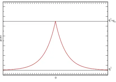
Such fluctuations can be for example spin-orbit couplings. An example is [21] where both, a Gaussian distribution and a Cusp are considered in a simulation. The autocorrelation assumed here is given as

g(∆t) = ¯ η ² + g 0 e ^−ν∆t = ¯ η ² + g 0 − g 0 ν|∆t| + g 0

2 ν ² |∆t| ² + O |∆t| ³

. (9)

The Taylor series expresses the autocorrelation in powers of |∆t|. This will play a role

in the chapters 1.2.3 and 1.2.4 because the conditions for pulses of the first two orders

are a consequence of the orders zero and one of this Taylor series. A special term in (9)

that we want to pay attention to is the term linear in |∆t| because this term concerns

the new investigations to which this work belongs to. This term is a special feature of a

cusp-like autocorrelation in comparison with a Gauß distribution. In many previous works

a Gauß distribution was used as the autocorrelation where the term does not exist due

to the vanishing derivation of a Gauß distribution in its maximum. The importance of

this term lies in the fact that it leads to an order in the Frobenius norm that was just in

[21] discovered. You can see the derivation of this order in chapter 1.2.3. A plot of the

autocorrelation can be seen in figure 1.

∆t

g( ∆ t)

0

η

+g

η

Figure 1: Cusp-like autocorellation in dependence of the time distance

1.2 Supression of decoherence

The aim of this chapter is to set up a quantitative definition of the pulse quality in terms of decoherence suppression. At first we set up the time evolution operator for the interaction between the central spin and the bath following the way of the calculations in [31]. This is needed in order to set up the so called Frobenius norm of a pulse. The Frobenius norm describes the difference between the actual pulse and the theoretically ideal pulse. The ideal pulse would be a delta peak [31] but it is not realizable in exper- iments because of its infinite big amplitude and its infinite short pulse duration. Hence the Frobenius norm is a quantification for the quality of a pulse and we get mathematical expressions which we need for the pulse search. The Frobenius norm will be expressed in orders of the pulse duration. The idea to let these orders vanish in ascending order leads to conditions that the pulses shall fulfill.

The shapes of the pulses, the conditions and the Frobenius norm will be expressed at first in dependence of the pulse duration. This is shiftable into expressions in dependence of the maximum amplitude or the energy of a pulse, so that the pulses are in every case expressed in dependence of one variable. The expressions in different variables are just different sights on the same pulse and do not mean a change of the physics. But an aspect which is physically important is the choice of the variable which we try to minimize. That means we search for a pulse which is good under the definition of quality that we set up in chapters 1.2.3 and 1.2.4 and in addition minimizes the value of one of the three variables.

The effect which we want to reach is that the pulse is optimized under a certain value of

1.2.1 Time evolution operator

To set up the time evolution operator we follow the calculations of [31]. The most general formulation of the time evolution operator over the whole pulse duration U _p (τ _p , 0) is given by

U p (τ p , 0) = e ^−iτ

^H

T{e ^{−i~ σ· R}

^{~ v(t)dt} }U _I (τ p , 0). (10) The first exponential function is the time evolution of the bath, the second exponential function is the time evolution induced by the pulse and U I (τ p , 0) is the time evolution induced by the interaction between the central spin and the bath which is the disturbing part in the system that we want to have as close to the identity operator as possible. The time evolution for the applied pulse P ˆ t can be rearranged as

P ˆ _t :=T {e ^{−i~ σ· R}

^{~ v(t}

^)dt

} (11)

=e ^{−i~ σ·ˆ a(t)}

.

This formulation represents a rotation around the pulse field in the rotating wave approxi- mation [32]. ˆ a(t) is the axis of rotation and ψ(t) is the angle of rotation. The Schrödinger equation for the pulse is

i∂ t P ˆ t = H P (t) ˆ P t . (12)

~

v(t) written in dependence of ~a(t) and ψ(t) is

2~ v(t) = ˙ ψ(t)~a(t) + ˙ ~a(t) sin ψ(t) − [1 − cos ψ(t)]

h ~a(t) ˙ × ~a(t) i

(13)

⇔ ~ v(t) · ~a(t) = ψ(t) ˙

2 . The calculations of (13) can be seen in detail in [25].

The total time evolution obeys the Schrödinger equation

i∂ t U p (t, 0) = [H B + H I + H P ] U p (t, 0) (14) From a combination of (12) and (14) we get

i∂ t U I (t, 0) = G(t)U I (t, 0) (15) G(t) = e ^iH

^t P ˆ _t ⁻¹ (~ σ · ~ η) ˆ P _t e ^−iH

^t (16) The Schrödinger equation (15) leads to the interaction part of the time evolution operator over the whole pulse duration

U I (τ p , 0) = T{e ^{−i R}

^G(t)dt }. (17)

Now we calculate the time evolution of the bath and the pulse separately. We define according to [31] H _qb

G(t) =e ^iH

^t H qb e ^−iH

^t (18)

H qb = ˆ P _t ⁻¹ (~ σ · ~ η) ˆ P t (19)

=~ σ · ~ η cos ψ(t) − ~ σ · [~a(t) × ~ η] sin ψ(t) + 2 [~a(t) · ~ η] [~ σ · ~a(t)] sin ² (ψ(t))

2 .

The calculations in (18) can be seen in detail in [31].

Further we define according to [31]

S(t) := ˆ ~ P _t ⁻¹ ~ σ P ˆ t = D _{ˆ a} (ψ)~ σ. (20) The meaning of (20) is that the influence of the pulse is captured in a rotation of the Pauli matrices vector ~ σ where D _{ˆ a} (ψ) is the corresponding 3 × 3 rotation matrix. Now we shift the expression of the rotation from the pauli matrices vector ~ σ to the field ~ η so that ~ σ will be static in our picture.

H _qb = ˆ P _t ⁻¹ (~ σ · ~ η) ˆ P _t = S(t)~ ~ η = [D _{ˆ a} (ψ)~ σ] · ~ η = [D _{ˆ a} (−ψ)~ η] ~ σ := ~ n _η (t) · ~ σ (21) (18) and (21) lead to

~ n _η (t) = ~ η cos ψ(t) − [~a(t) × ~ η] sin ψ(t) + ~a(t) [~a(t) · ~ η] [1 − cos ψ(t)] . (22) Now we include the time evolution of the bath into our calculations, e.g. we calculate G(t).

This has an effect only on η:

~

η(t) = ~ η _t = e ^iH

^t ~ ηe ^−iH

^t (23) As described in chapter 1.1.1 H B is captured in the time evolution of ~ η and hence H B

is henceforth no longer in our equations because this time evolution is replaced by the statistical noise model presented in chapter 1.1.2.

Now we want to transform (17) into a mathematical expression that we can work with in the pulse search. In order to do this we expand the exponent with a Magnus expansion.

The Magnus expansion builds up a power series expression of an exponent, in this case a series of powers of the pulse duration τ p . This is a description which is needed for the variational pulse search technique because we must be able to see the effect of a small variation on the pulse quality in a quantitative way. A detailed description such as a proof of the Magnus expansion can be seen in [33]. The Magnus expansion of (17) is given by

U (τ _p , 0) = e ⁻ⁱ

R

0

G(t)dt−

2

R

dt

R

0

dt

[G(t

),G(t

)]+O(τ

)

. (24)

If we insert G(t) = ~ n _η

(t) · ~ σ where η _t is the statistical fluctuating field, we get U(τ p , 0) =e ⁻ⁱ

R

0

~ n

(t)·~ σdt−

R

dt

R

0

dt

[ ^{~ n}

(t

)·~ σ,~ n

(t

)·~ σ ] ^+O(τ

)

(25)

=e ⁻ⁱ ( ^{~ µ}

^{·~ σ+~ µ}

^{·~ σ+O(τ}

⁾ ) .

We are interested in the first order of the Magnus expansion. The following calculations can be seen in detail in [25].

Now we calculate the first order of the Magnus expansion for amplitude-modulated pulses.

The axis of rotation is

~a(t) =





 0 1 0





 (26)

and (13) leads to the differential equation v(t) =

ψ(t) ˙

2 (27)

which is analytically solvable. The first order for amplitude-modulated pulses is

~

µ ⁽¹⁾ · ~ σ =

τ

Z

0

~ n _η (t ₁ ) · ~ σdt (28)

=σ _z

τ

Z

0

η(t) cos ψ(t)dt − σ _x

τ

Z

0

η(t) sin ψ(t)dt.

For frequency-modulated pulses the situation is more difficult. The axis of rotation is

~a(t) =







sin (θ(t)) cos (φ(t))) sin (θ(t)) sin (φ(t)))

cos (θ(t))





 . (29) and (13) leads to the system of equations

∂ψ(t)

∂t =2V 0 sin (θ(t)) [sin (Ω(t)) sin (φ(t)) + cos (Ω(t)) cos (φ(t))] (30)

∂φ(t)

∂t =V ₀

cos _ψ(t)

2

sin (Ω(t) − ψ(t)) − sin _ψ(t)

2

cos (θ(t)) cos (Ω(t) − φ(t)) sin _ψ(t)

2

sin (θ(t))

(31)

∂θ(t)

∂t =V ₀

cos _ψ(t)

2

cos (θ(t)) cos (Ω(t) − φ(t)) + sin _ψ(t)

2

sin (Ω(t) − ψ(t)) sin _ψ(t)

2

. (32)

The system of equations is not analytically solvable. This is a problem that makes the variational calculation for frequency-modulated pulses more complicated than the varia- tional calculation for amplitude-modulated pulses as you can see in chapter 4. θ(t) and φ(t) are functions, which appear because of the non-static rotation axis. These functions and ψ(t) are auxiliary functions which are not part of the underlying mathematical problem.

In theory the problem could be described completely without these functions, but these functions still stand as placeholders in the equations because there is no analytical solution of the system of the equations (30), (31) and (32). The first order for frequency-modulated pulses is according to [25]

~

µ ⁽¹⁾ · ~ σ =

τ

Z

0

~

n _η (t ₁ ) · ~ σdt (33)

=¯ ησ _x

τ

Z

0

(−a _y (t) sin (ψ(t)) + (1 − cos (ψ(t)))a _x (t)a _z (t)) dt

+ ¯ ησ y τ

Z

0

(a x (t) sin (ψ(t)) + (1 − cos (ψ(t)))a y (t)a z (t)) dt

+ ¯ ησ y τ

Z

0

cos (ψ(t)) + (1 − cos (ψ(t)))a ² _x (t) dt.

Because it is important in chapter 4, we write down the second order, too. It is

µ ⁽²⁾ =2i~ σ

τ

Z

0 t

Z

0

(~ n _η (t ₁ ) × ~ n _η (t ₂ )) dt ₂ dt ₁ (34)

=2iσ _x η ¯ ² + g ₀

τ

Z

0 t

Z

0

(n _yz (t ₁ )n _zz (t ₂ ) − n _zz (t ₁ )n _yz (t ₂ )) dt ₂ dt ₁

=2iσ y η ¯ ² + g 0

τ

Z

0 t

Z

0

(n zz (t 1 )n xz (t 2 ) − n xz (t 1 )n zz (t 2 )) dt 2 dt 1

=2iσ z η ¯ ² + g 0

τ

Z

0 t

Z

0

(n xz (t 1 )n yz (t 2 ) − n yz (t 1 )n xz (t 2 )) dt 2 dt 1

with the abbreviation

~ n _{~ η} (t) = η(t)







−a _y (t) sin (ψ(t)) + (1 − cos (ψ(t)))a _x (t)a _z (t)

−a _x (t) sin (ψ(t)) + (1 − cos (ψ(t)))a _y (t)a _z (t) cos (ψ(t)) + (1 − cos (ψ(t)))a ² _x (t)





 . (35)

1.2.2 Frobenius norm

After the calculation of the time evolution operator of the disturbance we follow a calculation of Stanek of which a short version can be found in [21] in order to get a quantified expression for the pulse quality. The deviation between the ideal pulse with the density matrix ρ ^γ _id and the real pulse with the density matrix ρ ^γ re is expressed in the density matrix

ρ ^γ :=ρ ^γ _id − ρ ^γ _re (36)

(37) with

ρ ^γ _id = ˆ P _τ

ρ ^γ ₀ P ˆ _τ ^†

(38) ρ ^γ _re = ˆ P _τ

U _I (τ _p )ρ ^γ ₀ U _I ^† (τ _p ) ˆ P _τ ^†

The density matrices ρ ^γ ₀ represent totally polarized states of the central spin in the direction of the axis γ. They are given by

ρ ^γ ₀ = 1

2 [ 1 + σ ^γ ] (39)

The square of the Frobenius norm ∆ F is defined as

∆ ² _F := 1 3

X

γ=x,y,z

T r (ρ ^γ ) ² . (40)

After carrying out the square and exploiting the properties of the time evolution and the rotation operator according to [21] (40) leads to

∆ ² _F := 2

"

1 − 1 3

X

γ=x,y,z

T r ρ ^γ _id ρ ^γ _re

#

. (41)

It is helpful to write the time evolution operators of the interaction as U _I (τ p ) = 1 · cos |~ µ| − i ~ µ · ~ σ

|~ µ| sin |~ µ|. (42) We will use

(σ γ (~ µ · ~ σ)) ² = µ ² _γ −

α6=γ

X

α=x,y,z

µ ² _α (43)

(~ µ · ~ σ) ² = |~ µ| ² (44)

T r

2σ γ (~ µ · ~ σ) ²

= 0. (45)

With these equations we calculate the trace in (41) using P ˆ τ ^†

P ˆ _τ

= 1 and cyclical permu- tation under the trace:

T r ρ ^γ _id ρ ^γ _re

=T r

P ˆ _τ

ρ ^γ ₀ P ˆ _τ ^†

P ˆ _τ

U _I (τ _p )ρ ^γ ₀ U _I ^† (τ _p ) ˆ P _τ ^†

(46)

= cos |~ µ| ² + sin ² |~ µ|

4|~ µ| ² · T r (~ µ · ~ σ) ² + 2σ γ (~ µ · ~ σ) ² + (σ γ (~ µ · ~ σ)) ²

= cos |~ µ| ² + sin ² |~ µ|

|~ µ| ² µ ² _γ We insert this trace into the Frobenius norm:

∆ ² _F =2

"

1 − 1 3

X

γ=x,y,z

T r ρ ^γ _id ρ ^γ _re

#

(47)

=2

"

1 − cos |~ µ| ² − 1 3

sin |~ µ| ²

|~ µ| ² µ ² _x + µ ² _y + µ ² _z

#

= 4 3

1 − cos ² |~ µ|

.

Until this point we have calculated the Frobenius norm exactly. Now we are going to make an approximation. We insert the Taylor series of the cosine into (47) and thus we get according to the calculations of Stanek

∆ ² _F ≈ 4 3

1 − (1 − 1 2 |~ µ| ² ) ²

= 4

3 |~ µ| ² + O |~ µ| ⁴

. (48)

In the next two sections we are going to deduce conditions for amplitude-modulated and

frequency-modulated pulses from (48) and from the boundary conditions.

1.2.3 Conditions for amplitude-modulated pulses

For the conditions we use just the first order of the Magnus expansion. We calculate the contribution of this order to ∆ _F by inserting it into (48) according to [25].

µ ⁽¹⁾ x

2 + µ ⁽¹⁾ z

2 (49)

=

τ

Z

0 τ

Z

0

g(t ₁ − t ₂ ) sin (ψ(t ₁ )) sin (ψ(t ₂ ))dt ₁ dt ₂

+

τ

Z

0 τ

Z

0

g(t ₁ − t ₂ ) cos (ψ(t ₁ )) cos (ψ(t ₂ ))dt ₁ dt ₂

=

τ

Z

0 τ

Z

0

g(t 1 − t 2 ) cos (ψ(t 1 ) − ψ(t 2 ))dt 1 dt 2

We insert the Taylor series (9) of the autocorrelation.

µ ⁽¹⁾ x

2 + µ ⁽¹⁾ z

2 (50)

=

τ

Z

0 τ

Z

0

¯

η ² + g ₀ − g ₀ ν|∆t| + g ₀

2 ν ² |∆t| ² + O |∆t| ³

cos (ψ(t ₁ ) − ψ(t ₂ ))dt ₁ dt ₂

Now there are different orders of |∆t|. Note that there are two reasons for different orders in

∆ F and their combination leads to the actual orders. One reason is the Magnus expansion of the time evolution operator and the other one is the Taylor series of the autocorrelation.

At first we look at the first order of the Taylor series. We set up the demand on the pulses that the order from the first order of the Magnus expansion and the first order of the Taylor series vanishes completely:

τ

Z

0 τ

Z

0

¯

η ² cos (ψ(t ₁ ) − ψ(t ₂ ))dt ₁ dt ₂ =0 (51)

¯ η ²





τ

Z

0

sin(ψ(t ₁ ))dt ₁

τ

Z

0

sin(ψ(t ₂ ))dt ₂ +

τ

Z

0

cos(ψ(t ₁ ))dt ₁

τ

Z

0

cos(ψ(t ₂ ))dt ₂



 =0

According to [25] we get the two conditions (52) and (53). Further we deduce a boundary condition from the usage of π-pulses [25]. We know that the difference between the initial angular ψ(0) and the final angular ψ(τ p ) has to be π and hence we can write down the condition (54).

τ

Z

0

sin (ψ(t))dt = 0 (52)

τ

Z

0

cos (ψ(t))dt = 0 (53)

ψ(τ _p ) − ψ(0) = π (54)

The biggest contribution to the decoherence on the central spin is due to the first order of the Frobenius norm. Thus the fulfillment of the conditions (52) and (53) is a reasonable first step in order to suppress decoherence. Further we look at the second order of the Taylor series in (50) and define

X = −

τ

Z

0 τ

Z

0

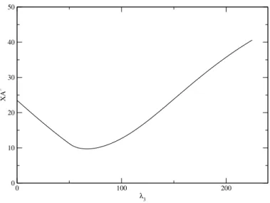
|t ₁ − t ₂ | cos (ψ(t ₁ ) − ψ(t ₂ ))dt ₁ dt ₂ . (55)

As explained in chapter 1.2.2 this term is a recently discovered [21] special feature of the

cusp-like autocorrelation in comparison with a Gauß distribution where this order does not

exist. The meaning of this term is that it is the order τ _p ³ with its prefactor in ∆ ² _F . After we

let the first order vanish via the conditions (52) and (53) it would be nice to let the second

order vanish, too. But this is not possible because of the No-Go theorem. It is shown in

[15] that it is impossible to let (55) vanish at the same time when the conditions (52), (53)

and (54) are fulfilled. Thus the best what we can try to reach is to create a pulse, which

makes (55) as small as possible while (52), (53) and (54) are fulfilled.

1.2.4 Conditions for frequency-modulated pulses

For frequency-modulated pulses we set up conditions in analogy to the condition for amplitude-modulated pulses such as in [25]. We use (33) to calculate

µ ⁽¹⁾ x

2 + µ ⁽¹⁾ y

2 + µ ⁽¹⁾ z

2 (56)

=

τ

Z

0 τ

Z

0

g(t ₁ − t ₂ ) (−a _y (t ₁ ) sin (ψ(t ₁ )) + (1 − cos (ψ(t ₁ )))a _x (t ₁ )a _z (t ₁ )) (−a _y (t 2 ) sin (ψ(t 2 )) + (1 − cos (ψ(t 2 )))a x (t 2 )a z (t 2 )) dt 1 dt 2

+

τ

Z

0 τ

Z

0

g(t ₁ − t ₂ ) (a _x (t ₁ ) sin (ψ(t ₁ )) + (1 − cos (ψ(t ₁ )))a _y (t ₁ )a _z (t ₁ )) (a _x (t ₂ ) sin (ψ(t ₂ )) + (1 − cos (ψ(t ₂ )))a _y (t ₂ )a _z (t ₂ )) dt ₁ dt ₂

+

τ

Z

0 τ

Z

0

g(t 1 − t 2 ) cos (ψ(t 1 )) + (1 − cos (ψ(t 1 )))a ² _x (t 1 ) cos (ψ(t ₂ )) + (1 − cos (ψ(t ₂ )))a ² _x (t ₂ )

dt ₁ dt ₂ . We insert the Taylor series (9):

µ ⁽¹⁾ x

2 + µ ⁽¹⁾ y

2 + µ ⁽¹⁾ z

2 (57)

=

τ

Z

0 τ

Z

0

¯

η ² + g 0 − g 0 ν|∆t| + g 0

2 ν ² |∆t| ² + O |∆t| ³ (−a _y (t ₁ ) sin (ψ(t ₁ )) + (1 − cos (ψ(t ₁ )))a _x (t ₁ )a _z (t ₁ )) (−a _y (t ₂ ) sin (ψ(t ₂ )) + (1 − cos (ψ(t ₂ )))a _x (t ₂ )a _z (t ₂ )) dt ₁ dt ₂ +

τ

Z

0 τ

Z

0

¯

η ² + g 0 − g 0 ν|∆t| + g 0

2 ν ² |∆t| ² + O |∆t| ³ (a _x (t ₁ ) sin (ψ(t ₁ )) + (1 − cos (ψ(t ₁ )))a _y (t ₁ )a _z (t ₁ )) (a _x (t ₂ ) sin (ψ(t ₂ )) + (1 − cos (ψ(t ₂ )))a _y (t ₂ )a _z (t ₂ )) dt ₁ dt ₂ +

τ

Z

0 τ

Z

0

¯

η ² + g 0 − g 0 ν|∆t| + g 0

2 ν ² |∆t| ² + O |∆t| ³ cos (ψ(t ₁ )) + (1 − cos (ψ(t ₁ )))a ² _x (t ₁ )

cos (ψ(t ₂ )) + (1 − cos (ψ(t ₂ )))a ² _x (t ₂ ) dt ₁ dt ₂

In analogy to the amplitude-modulated pulses we want to let the order from the first order

of the Magnus expansion and the first order of the Taylor series vanish. We derive the

first order conditions from (57). Further there are boundary conditions for the frequency-

modulated pulses which you can see in [25]. Altogether we get the following conditions:

τ

Z

0

(−a _y (t) sin (ψ(t)) + (1 − cos (ψ(t)))a _x (t)a _z (t)) dt = 0 (58)

τ

Z

0

(a x (t) sin (ψ(t)) + (1 − cos (ψ(t)))a y (t)a z (t)) dt = 0 (59)

τ

Z

0

cos (ψ(t)) + (1 − cos (ψ(t)))a ² _x (t)

dt = 0 (60)

ψ(τ _p ) − ψ(0) = π (61)

θ(τ p ) = π

2 (62)

∆ F in the second order of the Taylor series is derived in chapter 4 because it is a newly derived formula in this work.

2 Variational Calculation for Amplitude-Modulated Pulses

This chapter contains the central investigations of this work for amplitude modulated- pulses. At first we give an overview of the ansatz and start with the essential calculations of the variation in chapter 2.1 where we finally come to the central differential equation which we want to solve. This differential equation will be solved in two main steps. The first step is to set one Lagrange multiplier to zero and solve the remaining equation analytically in chapter 2.2. The second step is the extension of the solution to a solution of the general equation with a numerical method in chapter 2.3.

2.1 Variational ansatz

We start with an explanation of the variational ansatz. Our initial situation consists of

fulfillment of the conditions because of the No-Go Theorem [34]. Thus the best we can try to reach is to make X as small as possible while we fulfill the three conditions.

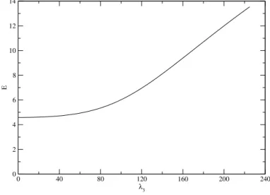
In addition to these aims stemming from the wanted pulse quality we want to set up a further aim which leads to a good realizability of the pulse in an experiment or further a device such as a quantum computer. Previous works such as [21] aim at a big pulse duration or a small amplitude. Both of these ideas are hardly integrable into our variational calculus due to the fact that it is difficult to include a discrete limitation of such values and thus we have to think about something different. The idea is to minimize the energy of a pulse given by

E = 1 2

Z τ

0

v ² (t). (63)

E and X can be minimized with different weightings to each other via a Lagrange multiplier that you will see in the formulas. The minimization of the energy is reasonable because of two aspects. The first one is that it can be beneficial to use pulses with a low energy due to a limited energy supply and heating. The second one is that the deviation of the actual spin angle ψ(t) ˙ which is contained in the energy corresponds to the amplitude of a pulse and thus we get a special form of an amplitude minimization in our method, too.

The energy is suitable to our variational calculation because we can insert it easily into the functional I. In total we have two terms X and E that we want to minimize while we want to fulfill the three conditions (52), (53) and (54). This is a typical optimization problem and a variational calculation is a good suggestion for the solution of such a problem.

A variational calculation is generally used to find the static points and thus the maxima, minima or saddle points of a functional I (~ q(t), ~ q, t). In the argument of the functional ˙ stand the functions ~ q(t), their first deviations ~ q(t) ˙ and the variable t. Hence the initial equation of a variational calculation is

δI(~ q(t), ~ q(t), t) = 0. ˙ (64) The functional is written as an integral over a Lagrange function L:

I = Z

L

~

q(t), ~ q(t), t ˙

dt. (65)

Finally the solutions are reached over the Euler-Lagrange equations for every single function q _i (t):

d dt

∂L

∂ q ˙ i (t) − ∂L

∂q i (t) = 0. (66)

2.1.1 Functional

Now we want to adjust our problem to a variational calculation as described above.

With (52), (53), (55) and (63) we define the functional

I = 1 8

τ

Z

0

ψ ˙ ² (t)dt + λ 1 τ

Z

0

sin (ψ(t))dt + λ 2 τ

Z

0

cos (ψ(t))dt (67)

+ λ ₃

τ

Z

0 τ

Z

0

|t ₁ − t ₂ | cos (ψ(t ₁ ) − ψ(t ₂ ))dt ₁ dt ₂ .

λ ₁ , λ ₂ and λ ₃ are Lagrange multipliers.

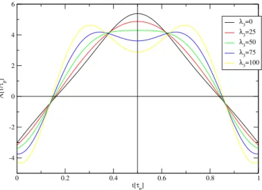
2.1.2 Lagrangian

To set up a Lagrangian at first we have to identify the coordinates and the variable in (65) for our problem. Our problem is one dimensional and thus there is just one Euler- Lagrange equation. The coordinate that we use is the angle ψ(t) depending on the variable t. Note that we are finally searching for a pulse shape defined by (27) which depends on ψ(t). This will play an important role later in this work because when we know any general ˙ solutions for ψ(t) depending on a number of variables the solutions for v(t) depend on one variable less because one variable gets lost by the derivation.

We set up the Lagrangian for our problem by identifying L in (65). This is easy for the three terms in (67) which consist of one integral where the terms contributing to the Lagrangian are just the integrands. For the term consisting of two integrals it is not that easy. It is easily comprehensible that one integral must stay in L after removing the integral which you see in (65) but we cannot just remove one of the two integrals to get the contribution to L. In fact both integrals are equal before a formulation such as L. This leads to a prefactor.

To get this prefactor we trace the mathematical derivation of the general Euler-Lagrange equations. We call the integrand of X

f (ψ(t 1 ), ψ(t ˙ 1 ), ψ(t 2 ), ψ(t ˙ 2 )) = |t ₁ − t 2 | cos (ψ(t 1 ) − ψ(t 2 )). (68)

Then we derive the Euler-Lagrange equation and we can identify the contribution to L.

δ

τ

Z

0 τ

Z

0

f(ψ(t 1 ), ψ(t ˙ 1 ), ψ(t 2 ), ψ(t ˙ 2 ))dt 1 dt 2 = 0 (69)

⇔

τ

Z

0 τ

Z

0

f(ψ(t ₁ ) + δψ(t ₁ ), ψ(t ˙ ₁ ) + δ ψ(t ˙ ₁ ), ψ(t ₂ ) + δψ(t ₂ ), ψ(t ˙ ₂ ) + δ ψ(t ˙ ₂ ))

−f (ψ(t ₁ ), ψ(t ˙ ₁ ), ψ(t ₂ ), ψ(t ˙ ₂ ))

dt ₁ dt ₂ = 0

⇔

τ

Z

0 τ

Z

0

∂f

∂ψ(t ₁ ) δψ(t 1 ) + ∂f

∂ ψ(t ˙ ₁ ) δ ψ(t ˙ 1 ) + ∂f

∂ψ(t ₂ ) δψ(t 2 ) + ∂f

∂ ψ(t ˙ ₂ ) δ ψ(t ˙ 2 )

dt 1 dt 2 = 0

⇔

τ

Z

0 τ

Z

0

∂f

∂ψ(t ₁ ) δψ(t ₁ )dt ₁ dt ₂ +

τ

Z

0

δψ(t ₁ ) ∂f

∂ ψ(t ˙ 1 ) τ

0

dt ₂ −

τ

Z

0 τ

Z

0

δψ(t ₁ ) d dt ₁

∂f

∂ ψ(t ˙ 1 ) dt ₁ dt ₂

τ

Z

0 τ

Z

0

∂f

∂ψ(t 2 ) δψ(t ₂ )dt ₁ dt ₂ +

τ

Z

0

δψ(t ₂ ) ∂f

∂ ψ(t ˙ 2 ) τ

0

dt ₁ −

τ

Z

0 τ

Z

0

δψ(t ₂ ) d dt 2

∂f

∂ ψ(t ˙ 2 ) dt ₁ dt ₂ = 0

⇔

τ

Z

0 τ

Z

0

∂f

∂ψ(t 1 ) δψ(t 1 ) + δψ(t 1 ) d dt 1

∂f

∂ ψ(t ˙ ₁ )

dt 1 dt 2

+

τ

Z

0 τ

Z

0

∂f

∂ψ(t ₂ ) δψ(t 2 ) + δψ(t 2 ) d dt ₂

∂f

∂ ψ(t ˙ ₂ )

dt 1 dt 2 = 0

The single integrals in the last step vanish due to the fact that δψ(t) is zero in the starting and the ending point t = 0 and t = τ _p . The integrands are completely symmetrical in t ₁ and t ₂ because X is symmetrical in t ₁ and t ₂ as you can see in (55). Further the range of integration is equal for t 1 and t 2 and hence we get:

τ

Z

0 τ

Z

0

∂f

∂ψ(t 1 ) δψ(t ₁ ) + δψ(t ₁ ) d dt 1

∂f

∂ ψ(t ˙ 1 )

dt ₁ dt ₂ (70)

=

τ

Z

0 τ

Z

0

∂f

∂ψ(t 2 ) δψ(t 2 ) + δψ(t 2 ) d dt 2

∂f

∂ ψ(t ˙ ₂ )

dt 1 dt 2 .

Thus we can write:

δ

τ

Z

0 τ

Z

0

f (ψ(t 1 ), ψ(t ˙ 1 ), ψ(t 2 ), ψ(t ˙ 2 ))dt 1 dt 2 (71)

=2

τ

Z

0 τ

Z

0

∂f

∂ψ(t ₁ ) δψ(t ₁ ) + δψ(t ₁ ) d dt ₁

∂f

∂ ψ(t ˙ 1 )

dt ₁ dt ₂

=

τ

Z

0











∂

2

τ

R

0

f dt ₂

∂ψ(t ₁ ) δψ(t 1 ) + δψ(t 1 ) d dt

∂

2

τ

R

0

f dt ₂

∂ ψ(t ˙ ₁ )









 dt 1 .

Now we can identify the contribution to L in comparison with (65) as

L _X (ψ(t), ψ(t), t) = 2 ˙

τ

Z

0

f dt ₂ = 2

τ

Z

0

|t − t ₂ | cos (ψ(t) − ψ(t ₂ ))dt ₂ . (72)

Then we have all the terms that we need to write down the Lagrangian as

L(ψ(t), ψ(t), t) ˙ (73)

= 1

8 ψ(t) ˙ ² + λ ₁ sin (ψ(t)) + λ ₂ cos (ψ(t)) + 2λ ₃

τ

Z

0

|t − t ₂ | cos (ψ(t) − ψ(t ₂ ))dt ₂ .

2.1.3 Euler-Lagrange equation

The next step is to derive the Euler-Lagrange equation from the Lagrangian. We insert (73) into (66):

d dt

∂L(ψ(t), ψ(t), t) ˙

∂ ψ(t) ˙ − ∂L(ψ(t), ψ(t), t) ˙

∂ψ(t) = 0 (74)

d dt

∂ ¹ ₈ ψ ˙ ² (t)

∂ ψ(t) ˙ −

∂

λ ₃ 2

τ

R

0

|t − t ₂ | cos (ψ(t) − ψ(t ₂ ))dt ₂ + λ ₁ sin (ψ(t)) + λ ₂ cos (ψ(t))

∂ψ(t) = 0

ψ ⁰⁰ (t) + 8λ ₃

τ

Z

0

|t − t ₁ | sin (ψ(t) − ψ(t ₂ ))dt ₂ + 4λ ₂ sin (ψ(t)) − 4λ ₁ cos (ψ(t)) = 0.

Now we want to capture the last two terms within one term. We calculate:

λ 2 sin (ψ(t)) − λ 1 cos (ψ(t)) (75)

= − λ ₂ i 2

e ^iψ(t) − e ^−iψ(t) + λ ₂ 1

2

e ^iψ(t) − e ^−iψ(t)

= − 1

2 (λ ₂ + iλ ₁ ) e ^iψ(t) − 1

2 (λ ₂ − iλ ₁ ) e ^−iψ(t)

= λ 2

2 s

1 + λ ² ₁ λ ² ₂

1 + i ^λ _λ

2

r 1 + ^λ _λ

2

e ^iψ(t) + λ 2

2 s

1 + λ ² ₁ λ ² ₂

1 − i ^λ _λ

2

r 1 + ^λ _λ

2

e ^−iψ(t)

= λ 1

2 s

1 + λ ² ₁ λ ² ₂ e ⁱ

ψ(t)+arctan

2

+ λ 2

2 s

1 + λ ² ₁ λ ² ₂ e ⁻ⁱ

ψ(t)+arctan

2

= q

λ ² ₂ + λ ² ₁ cos

ψ(t) + arctan λ 1

λ 2

= q

λ ² ₂ + λ ² ₁ sin

ψ(t) + arctan λ 1

λ ₂ + π 2

Thus we can rewrite (74) as:

ψ(t) + 4 ¨ q

λ ² ₂ + λ ² ₁ sin

ψ(t) + arctan λ ₁ λ 2

+ π 2

(76) + 8λ ₃

τ

Z

0

|t − t ₂ | sin (ψ(t) − ψ(t ₂ ))dt ₂ = 0

Before we start to solve the Euler-Lagrange equation (76) we want to think about a few general aspects of the solutions and the physical meaning of these aspects.

(76) is a differential equation of the second order. This means that the solution for ψ(t) contains two integration constants which will be variables in the solution. Further there are three Lagrange multipliers in (76) and thus these three Lagrange multipliers are variables in the solution, too. Hence altogether there are five variables in the general solution for ψ(t).

But an important point is that in the end we are not searching for a solution of ψ(t). We are searching for a solution of the pulse shape v(t) which is defined by (27) in dependence of the derivation ψ(t). This is important because one of the variables in the solution gets ˙ lost due to the derivation and thus the solution of v(t) contains just four variables.

Then an adjustment of the solution to the auxiliary conditions is necessary. Every auxil- iary condition determines one of the variables. Hence after adjusting the solution to the auxiliary conditions three variables are determined and just one free variable is left in the solution.

But because of the way in which we express the solution this variable will not appear in

our equation. We will choose specific values for λ ₃ and we will plot the functions that we

want to investigate against λ 3 . This means we just look at solutions for fix values of λ 3 .

For a fix value of λ 3 the solutions depend on no further variables. But this does not mean

that there is just one solution for a fix value of λ ₃ because different solutions in discrete

steps are possible. This stems from the discrete different possibilities to adjust the general

solution to the auxiliary conditions. The different discrete solutions will play an important role in this work because we will look at first at the symmetric solution which is one of these discrete solutions but rather we look at asymmetric solutions which are further solutions of these discrete steps.

Another important aspect is the meaning of λ 3 . This Lagrange multiplier is the weighting of X against the energy E in the minimization. This means if we choose λ 3 to be zero and we solve (76), we get the pulses with a minimized energy but there is absolutely no minimization of the term X. If we make λ 3 bigger we get pulses with a mix of a minimized energy E and the minimized term X. The bigger λ 3 is the stronger is the minimization of X in comparison with the minimization of E. If we let λ ₃ grow to infinity we reach the opposite case of λ 3 = 0 asymptotically. In this case we get a pulse with the minimized function X but almost no minimization of the energy E is included in our calculation.

In the differential equation (76) you can see a periodicity in ψ(t) with the period 2π.

This means the differential equation stays exactly the same if we add a phase of 2π to the function ψ(t).

Now we want to solve the Euler-Lagrange equation while we fulfill the conditions (52), (53) and (54). This is a typical optimization problem known from mathematics.

The best what we can try to reach is to get an analytical solution because in comparison to a numerical solution it delivers a formula as the solution which gives us more general information.

The problem is that (76) is to our knowledge not analytically solvable. The main prob- lem which prevents us from finding an analytical solution is the term with the integral.

Without this term (76) would be analytically solvable. Because we prefer an analytical solution to a numerical one it seems to be a good idea to solve as much of (76) as we can analytically and include the rest numerically into the solution. That means concretely that we want to solve the equation in the following two steps. In the first step we ignore the difficult term with the integral by setting λ ₃ = 0 and thus we get the differential equation:

ψ(t) + 4 ¨ q

λ ² ₃ + λ ² ₂ sin

ψ(t) + arctan λ ₂ λ 3

+ π 2

= 0 (77)

or with other constants λ and Φ corresponding to the amplitude and the angular in polar coordinates:

ψ(t) + 4λ ¨ sin

ψ(t) + Φ + π 2

= 0. (78)

This term is a form of the Sine-Gordon equation. We solve this equation analytically.

Further we have to adjust the solution to the auxiliary conditions (52), (53) and (54). This

is done in chapter 2.2.2. The analytical solution is not just a preparation step in order to

solve the general Euler-Lagrange equation (76), but rather it has an own physical meaning