Professur für Demografie Professorship of Demography
The choice of indicators influences conclusions about the educational gradient of sex-specific alcohol consumption
Florian Schulz, Jörg Wolstein, & Henriette Engelhardt
Otto-Friedrich-Universität Bamberg
University of Bamberg Demographic
Discussion Papers No. 21/2019
https://doi.org/10.20378/irbo-55267
THE CHOICE OF INDICATORS INFLUENCES CONCLUSIONS ABOUT THE EDUCATIONAL GRADIENT OF SEX-SPECIFIC ALCOHOL CONSUMPTION
Florian Schulz, Jörg Wolstein, & Henriette Engelhardt
June 2019
ABSTRACT
There has been considerable public interest in reports on harmful alcohol consumption of higher educated females. This study assesses the robustness of this finding with representative German data using ten different indicators of alcohol consumption. This cross-sectional study used data of the Epidemiological Survey on Substance Abuse from 2012. 4,225 females and 3,239 males represent the German population aged 18–64. It presents ten indicators of alcohol consumption by sex and education and provides group specific means and 95 %-confidence intervals. The main results are: (1) Higher educated males and females are drinking alcohol more frequently than lower educated males and females. (2) When drinking, higher educated males and females tend to drink less alcohol than lower educated males and females. (3) Only when using an indicator for hazardous alcohol consumption with different thresholds for males and females, the results indicate a pattern that significantly exposes hazardous alcohol consumption in the group of higher educated females. Concerning the choice of indicators, this study shows that sex-specific threshold-based indicators of alcohol consumption may lead to different conclusions as the majority of other indicators.
KEY WORDS
Alcohol | sex | education | indicators | hazardous drinking
INTRODUCTION
There has been considerable public interest (e.g. The Guardian 2015) in the findings of the OECD (2015) report on “Tackling Harmful Alcohol Use” regarding harmful alcohol
consumption of higher educated females. According to the report, the effect of education on hazardous alcohol consumption is much more pronounced in females than in males. In the scientific literature, by and large, social gradients of alcohol consumption differ for males and females and by educational levels (e.g. Bloomfield et al., 2006; Droomers, Schrijvers, and Mackenbach, 2004; Huckle, You, and Casswell, 2010; Pabst, Kraus, Gomes de Matos, and Piontek, 2013; van Oers et al., 1999). However, there is mixed evidence regarding the direction of the effects and the effect sizes.
For example, van Oers et al. (1999) and Droomers et al. (1999) reported no significant associations between education and excessive drinking behavior of females but a significantly higher prevalence of this pattern for lower educated males. However, Huckle et al. (2010) reported significant relations between females’ and males’ frequency of drinking and typical occasion quantities, stating that both females and males with higher education drink
significantly less alcohol per occasion but also have a significantly higher frequency of drinking alcohol.
The OECD report (2015) defined hazardous alcohol consumption as exceeding a sex- specific threshold of 21 units of alcohol or more for males, or 14 or more for females.
However, many studies used other criteria for hazardous alcohol consumption, e.g. using consumption measures without defining thresholds or with thresholds that were not sex- specific. In our study, we therefore use various definitions of the hazardous use of alcohol to assess the sex-specific effect of education on alcohol consumption in a representative German sample of males and females.
We contribute to this debate by estimating the prevalence of alcohol consumption with ten different indicators by sex and education using current representative data for Germany, testing the “robustness” of the results over these different consumption indicators.
METHODS
Data and sample
We used data from the Epidemiological Survey on Substance Abuse (ESA) of 2012, which is a nationally representative German sample on substance consumption, substance-related problems and their consequences (Kraus et al., 2013; Pabst et al., 2013; Steppan, Piontek, &
Kraus, 2014). The survey includes 9,081 respondents between 18 and 64 years of age. After dropping cases with missing information for sex, education or with non-German nationality (to reduce cultural heterogeneity), 7,464 respondents remain for the analyses. We applied the probability-weights provided in the data to uphold representativeness of the German
population.
Measures of alcohol consumption
In ESA, alcohol consumption is measured with a quantity-frequency-approach (Gmel &
Rehm, 2004). The respondents reported the number of drinking days within the last 30 days before the interview and the average units of beer, wine, liquor or other alcoholic beverages on each day they were drinking the respective beverage. Using beverage-specific alcoholic strengths per beverage (Kraus et al., 2014), the total amount of pure ethanol per month per respondent was calculated.
From this frequency and quantity information, we calculated ten indicators of alcohol consumption. frequency indicators (indicators 1-3), quantity and quantity-frequency
indicators (indicators 4-7), and indicators that are based on the assumption of physiological
indicates which indicators are based on thresholds and sex-specific assumptions, and shows descriptive statistics of each indicator.
--- Table 1 ---
The single indicators of alcohol consumption are: (1) abstinence during the last 30 days before the interview, as reported by the respondents in the questionnaire; (2) number of drinking days during the last 30 days before the interview, as reported by the respondents; (3) number of days with five or more glasses of alcohol (“binge drinking”) within the last 30 days, as reported by the respondents; (4) calculated average amount of pure ethanol per day as total amount of pure ethanol during the last 30 days divided by 30 (one respondent with more than 1,000 grams was dropped); (5) calculated average amount of pure ethanol per drinking day as total amount of pure ethanol during the last 30 days divided by the number of drinking days; (6) calculated weight adjusted pure ethanol per day as the total amount of pure ethanol per day divided by the respondents’ body weight in kilograms; (7) calculated weight adjusted pure ethanol per drinking day as the total amount of pure ethanol per month divided by the respondents’ body weight in kilograms and the number of drinking days; (8) calculated blood alcohol content per drinking day using Widmark’s formula (1932) with ‘Widmark factors’ of 0.7 for males and 0.6 for females on the basis of the self-reported number of
drinking days; risky drinking behavior, (9) if males and females consumed more than 24 or 12 grams of pure ethanol on average per day, respectively (guideline for low-risk drinking in Germany; Burger et al., 2004 – for comparison: roughly 0.6 liters of beer or 0.25 liters of wine contain 24g of ethanol), calculated from the total amount of pure ethanol per month, and (10) if males and females consumed more than 16 grams of pure ethanol on average per day (Department of Health, 2016).
Stratification variables
All estimates of alcohol consumption were stratified by respondents’ sex, educational level, age and squared age. All are measured as reported by the respondents in the questionnaire.
Highest attained educational level is based on the updated CASMIN classification (Brauns, Scherer, & Steinmann, 2003), which has proven to capture the educational gradient in different domains of everyday life, discerning three categories: tertiary qualification (labeled
“high”), intermediate or maturity qualification (labeled “medium”), and qualification below the intermediate level (labeled “low”). Table 2 shows case numbers and descriptives of the stratification variables, separately for males and females.
--- Table 2 ---
Analyses
We calculated the predicted prevalence of each of the ten drinking patterns by sex and education, as it is common in alcohol research (van Oers et al., 1999; Blomfield et al., 2006).
In Figures 1-3, we presented group specific means and 95%-confidence intervals for each combination of sex and education.
The predicted probabilities, frequencies, or quantities were derived as margins at the means (Williams, 2012) from the appropriate regression models in Tables A1, A2. The predictions were adjusted by setting all independent variables to the sample means. We estimated separate models for females and males. We used binary logistic regression models to predict the probabilities of abstinence (indicator 1), and the two versions of risky daily consumption (indicators 8, 9). We used negative binomial regression models to predict the frequencies of drinking days (indicator 2) and binge drinking days (indicator 3). We used linear regression models to predict the quantities of alcohol consumption (indicators 4, 5, 6, 7, 10). For all analyses of drinking frequency or quantity, we excluded abstainers. This is
common in the literature on drinking patterns, as the explanation of being abstinent has been found to be different from the explanation of different levels of drinking (Kuntsche et al., 2012).
We ran several sensitivity analyses to ensure the robustness of our results using different modeling approaches, control variables and samples restrictions. Most notably, we included abstainers in the models of drinking frequency and quantity. None of the sensitivity analyses showed substantially different results.
RESULTS
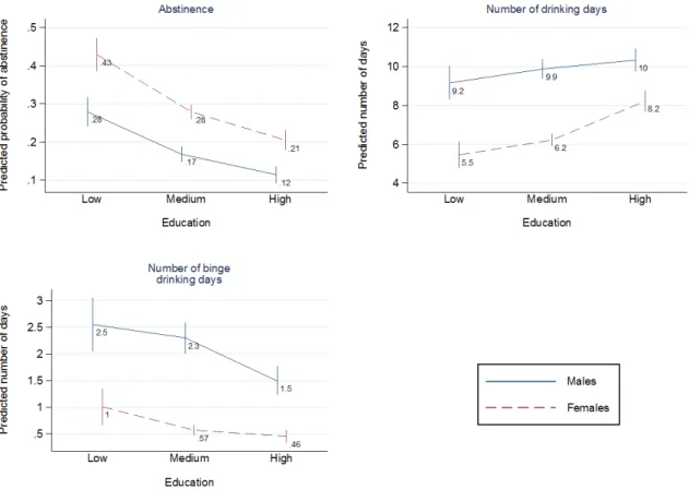
Figure 1 shows higher abstinence rates for females than for males in all three educational groups as well as higher abstinence rates for lower than for medium than for higher educated females and males. Males’ average number of drinking days within the last 30 days before the survey are significantly higher than females’ in all educational groups. For both females and males, lower and medium educational levels are not significantly different from each other.
For males, the number of drinking days is significantly higher for the higher educated than for the medium educated; higher educated females have a significantly higher drinking frequency than both medium and lower educated females. Lower and medium educated males have, on average, the highest number of days on which they drink five or more glasses of alcoholic beverages. Within all three groups of education, males’ average is significantly higher than females’. For both males and females, there is a significant difference only between medium and higher education.
--- Figure 1 ---
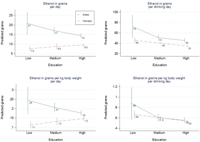
Figure 2 shows that the total calculated amount of pure ethanol per day and per drinking day is higher for male than for female respondents. There are no significant differences between
educational groups for females and males regarding ethanol consumption per day. Highly educated females, however, record the least calculated ethanol per drinking day compared to lower or medium educated females; the same association with education is found within the group of males. In all three educational groups, males record significantly higher amounts of pure ethanol per kilogram of body weight than females. For males, there are significant differences between the medium and the higher educated groups, for females between the lower and higher educated groups for ethanol in grams per kilogram body weight per day. The differences between males’ and females’ levels of weight-adjusted ethanol disappear if
analyzed for drinking days. Again, the associations within the two sex-groups are identical as higher educated significantly differ from lower and medium educated males as well as
females.
--- Figure 2 ---
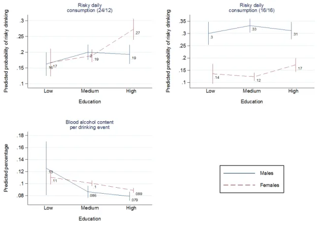
Figure 3 shows the average calculated blood alcohol content of females and males per drinking event: higher educated females have a significantly higher average than higher educated males. Again, the differences regarding education are the same within all males and females: higher educated have significantly lower averages of blood alcohol content than both lower and medium educated.
--- Figure 3 ---
Risky alcohol consumption – applying version (a) with thresholds of 24 g for males and 12 g for females – is more prevalent for higher educated females than for higher educated males as well as for all other combinations of sex and education. This is the only striking exception from the previous indicators as females show a clearly different pattern than males.
Changing the thresholds of risky drinking behavior to version (b)’s 16 g for both males and females changes the picture completely as, first, the prevalence for higher educated females
clearly decreases and, second, the prevalence of higher educated females is no longer significantly differs from lower educated females but still slightly differs from females with medium education.
DISCUSSION
Using a nationally representative sample of 7,464 German females and males, we presented a comparison of ten different indicators to measure alcohol consumption depending on sex and education. Nine out of ten indicators showed rather robust results regarding the education gradient of alcohol consumption for males and females. On the whole, we showed that higher educated males and females are drinking alcohol more frequently than lower educated males and females. When drinking, higher educated males and females tend to drink less alcohol or at least do not consume significantly different amounts of alcohol than lower educated males and females. . Only when using an indicator for hazardous alcohol consumption with different thresholds for males and females, our results indicated a pattern that significantly exposed hazardous alcohol consumption in the group of higher educated females, as did the OECD (2015) report.
The definition of thresholds for low-risk drinking is part of a long tradition in drinking guidelines. These guidelines have been established as a prevention tool in many countries (overview in House of Commons Science and Technology Committee, 2012) but the definition of limits varies largely (Harding & Stockley, 2007, Furtwaengler & de Visser, 2013) and often lacks clear scientific evidence (Rehm & Patra, 2012). Moreover, there is no consent, whether different limits of alcohol consumption should be recommended for males and females. Traditionally, lower limits of alcohol consumption were recommended for females than for males (e.g. 12 g/day for females and 24 g/day for males in Germany; Burger et al. 2004, Gomes de Matos et al., 2016), and this still shows in many national guidelines
of guidelines now recommend the same limits for both females and males (Department of Health 2016, Room & Rehm, 2012). Although they are meant as an educational prevention measure, the impact of such guidelines on drinking behavior is unclear (WHO 2007).
Moreover, drinking guidelines were perceived as having little relevance and were generally disregarded by lay people (Lovatt et al., 2015). However, they have been used to define thresholds of hazardous drinking and thus identify persons at risk in epidemiological studies.
In these cases, one may assume that results may vary remarkably, especially if sex-effects are at question, depending on which guideline is used.
In our study we showed that by using a different threshold for the definition of hazardous alcohol use (12 g/day for females, 24 g/day for males, Burger et al. 2004, Gomes de Matos et al., 2016), highly educated females not only showed higher risks attributable to alcohol as compared to males, but also as compared to females with medium or low
education. In contrast, when defining the threshold equally at 16 grams per day for males and females, as was done in the current guidelines of the UK Department of Health (2016), females showed generally less problematic alcohol use than males, and there was no significant difference between low and medium as well as low and high educated females.
Two possible limitations of the empirical design have to be considered: first, all estimates are based on self-reported measures of alcohol consumption which may be prone to measurement bias (Devaux & Sassi 2015). Second, our analyses are based on one single but nationally representative survey of German females and males aged 18–64 years. As for all studies of this kind, replications with other surveys have to contest our results.
We conclude from our study, first, that the education gradient of sex-specific alcohol consumption is not as large as shown in OECD (2015). Second, only when using the sex- specific threshold-indicator to flag risky drinking behavior, we were able to replicate the finding in OECD (2015) that high educated women are a high-risk group. Third, if there are differences between varying educational levels, these differences are rather related to
consumption patterns, i.e. the higher educated are drinking more frequently but consume lower quantities.
Concerning measurement and the choice of indicators, we conclude that it is not advisable to apply sex-specific threshold-based indicators as sole indicators of alcohol consumption. If sex-specific threshold-based indicators are of particular importance for whatever reason, we recommend embedding them in several other indicators as the majority of other indicators tell a different or much less pronounced story.
REFERENCES
Bloomfield K, Grittner U, Kramer S, Gmel, G. Social inequalities in alcohol consumption and alcohol-related problems in the study countries of the EU concerted action ‘Gender, Culture and Alcohol Problems: A multi-national study’. Alcohol Alcoholism 2006;41;i26–i36.
Brauns H, Scherer S, Steinmann S. The CASMIN educational classification in international comparative research. In Wolf C, editor. Advances in Cross-National Comparison. An European Working Book for Demographic and Socio-Economic Variables.
Amsterdam: Kluwer, 2003:196-221.
Burger M, Brönstrup A, Pietrzik K, Derivation of tolerable upper alcohol intake levels in Germany: a systematic review of risks and benefits of moderate alcohol consumption.
Prev Med 2004;39:111–27.
Department of Health. Alcohol Guidelines Review – Report from the Guidelines
Development Group to the UK Chief Medical Officers. UK Department of Health, https://www.gov.uk/government/uploads/system/uploads/attachment_data/file/545739/
GDG_report-Jan2016.pdf [March 15, 2017], 2016.
Devaux, M, Sassi, F. Social disparities in hazardous alcohol use: self-report bias may lead to incorrect estimates. Eur J Public Health 2015;26:129–34.
Droomers M, Schrijvers CTM, Mackenbach JP. Educational differences in starting excessive alcohol consumption: explanations from the longitudinal GLOBE study. Soc Sci Med 2003;58:2023–33.
Furtwaengler NA, de Visser RO. Lack of international consensus in low-risk drinking guidelines. Drug Alcohol Rev 2013;32:11–8.
Gmel G, Rehm J. Measuring alcohol consumption. Contemp Drug Probl 2004;34:467–540.
Gomes de Matos E, Atzendorf J, Kraus L, Piontek D. Substanzkonsum in der Allgemeinbevölkerung in Deutschland. Ergebnisse des Epidemiologischen Suchtsurveys 2015. Sucht 2016;62:271–81.
Harding, R, Stockley, CS. Communicating through government agencies. Ann Epidemiol 2007;17:S98–S102.
House of Commons Science and Technology Committee (2012) Alcohol guidelines. Eleventh Report of Session 2010–12. London: The Stationery Office Limited,
https://www.publications.parliament.uk/pa/cm201012/cmselect/cmsctech/1536/1536.p df [March 15, 2017].
Huckle T, You RQ, Casswell S. Socio-economic status predicts drinking patterns but not alcohol-related consequences independently. Addiction 2010;105:1192–202.
Kraus L, Piontek D, Pabst A, Gomes de Matos E. Studiendesign und Methodik des Epidemiologischen Suchtsurveys 2012. Sucht 2013;59:309–20.
Kraus L, Pabst A, Gomes de Matos E, Piontek D. Kurzbericht Epidemiologischer
Suchtsurvey. Tabellenband: Trends der Prävalenz des Alkoholkonsums, episodischen Rauschtrinkens und alkoholbezogener Störungen nach Geschlecht und Alter 1997–
2012. München: IFT Institut für Therapieforschung, 2014.
Kuntsche S, Knibbe RA, Kuntsche E, Gmel, G. Housewife of working mom – each to her own? The relevance of societal factors in the association between social roles and alcohol use among mothers in 16 industrialised countries. Addiction 2011;106:1925–
32.
Lovatt M, Eadie D, Meier PS, Li J, Bauld L, Hastings G, Holmes J. Lay epidemiology and the interpretation of low-risk drinking guidelines by adults in the United Kingdom.
Addiction 2015;110:1912–19.
OECD. Tackling Harmful Alcohol Use: Economics and Public Health Policy. OECD Publishing, 2015. DOI: 10.1787/9789264181069-en
Pabst A, Kraus L, Gomes de Matos E, Piontek D. Substanzkonsum und substanzbezogene Störungen in Deutschland im Jahr 2012. Sucht 2013;59:321–31.
Rehm, J, Patra, J. Different guidelines for different countries? On the scientific basis of low- risk drinking guidelines and their implications. Drug Alcohol Rev 2012;31:156–61.
Room R, Rehm J. Clear criteria based on absolute risk: Reforming the basis of guidelines on low‐risk drinking. Drug Alcohol Rev 2012;31:135–140.
Steppan M, Piontek D, Kraus L. The effect of sample selection on the distinction between alcohol abuse and dependence. Int J Alcohol Drug Res 2014;3:159–68.
The Guardian. Better-educated women contributing to rise in UK alcohol consumption – OECD Study finds better-educated men more likely to drink hazardous amount than less-educated counterparts, but difference much more pronounced for women.
https://www.theguardian.com/society/2015/may/12/better-educated-women- contributing-to-rise-in-uk-alcohol-consumption-oecd [December 01, 2017], 2015.
van Oers JAM, Bongers IMB, van de Goor LAM, Garretsen HFL. Alcohol consumption, alcohol-related problems, problem drinking, and socioeconomic status. Alcohol Alcoholism 1999;34:78–88.
WHO. WHO Expert Committee on Problems Related to Alcohol Consumption. Second report. World Health Organ Tech Rep Ser 2007;944: 1–53.
Widmark EMP. Die theoretischen Grundlagen und die praktische Verwendbarkeit der gerichtlich-medizinischen Alkoholbestimmung. Berlin: Urban und Schwarzenberg, 1932.
Williams, R. Using the margins command to estimate and interpret adjusted predictions and marginal effects. The Stata Journal 2012;12:308–331. http://www.stata-
journal.com/sjpdf.html?articlenum=st0260 [February 14, 2019].
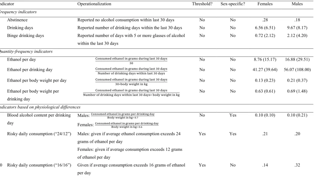
Table 1. Summary of the 10 indicators, and descriptives by respondents’ sex
Indicator Operationalization Threshold? Sex-specific? Females Males
Frequency indicators
1 Abstinence Reported no alcohol consumption within last 30 days No No .28 .18
2 Drinking days Reported number of drinking days within the last 30 days No No 6.56 (6.51) 9.67 (8.17)
3 Binge drinking days Reported number of days with 5 or more glasses of alcohol within the last 30 days
No No 0.72 (2.12) 2.12 (4.20)
Quantity-frequency indicators
4 Ethanol per day Consumed ethanol in grams during last 30 days
30 No No 8.76 (15.17) 16.88 (29.51)
5 Ethanol per drinking day Consumed ethanol in grams during last 30 days
Number of drinking days within last 30 days No No 41.27 (39.64) 56.07 (108.00) 6 Ethanol per body weight per day Consumed ethanol in grams during last 30 days
30∗body weight in kg No No 0.13 (0.23) 0.21 (0.37)
7 Ethanol per body weight per drinking day
Consumed ethanol in grams during last 30 days
Number of drinking days within last 30 days∗ body weight in kg No No 0.63 (0.61) 0.69 (1.48) Indicators based on physiological differences
8 Blood alcohol content per drinking day
Males: Consumed ethanol in grams per drinking day Body weight in kg∗ 0.7
Females: Consumed ethanol in grams per drinking day Body weight in kg∗ 0.6
No Yes 0.10 (0.10) 0.10 (0.21)
9 Risky daily consumption (“24/12”) Males: given if average ethanol consumption exceeds 24 grams of ethanol per day
Females: given if average consumption exceeds 12 grams of ethanol per day
Yes Yes .21 .20
10 Risky daily consumption (“16/16”) Given if average consumption exceeds 16 grams of ethanol per day
Yes No .14 .32
Note: Own compilation. Means/percentages and standard deviations (in parentheses). Epidemiological Survey on Substance Abuse 2012.
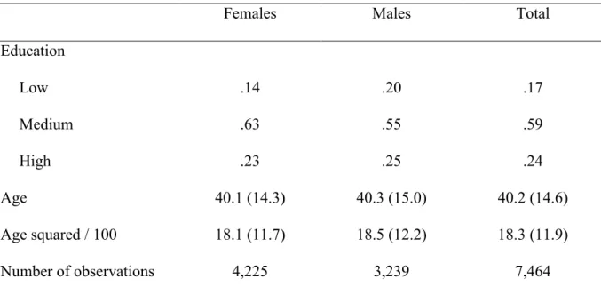
Table 2. Sample descriptives by respondents’ sex
Females Males Total
Education
Low .14 .20 .17
Medium .63 .55 .59
High .23 .25 .24
Age 40.1 (14.3) 40.3 (15.0) 40.2 (14.6)
Age squared / 100 18.1 (11.7) 18.5 (12.2) 18.3 (11.9)
Number of observations 4,225 3,239 7,464
Note: Case numbers, percent (education), means (age, age squared), standard deviations in parentheses. Epidemiological Survey on Substance Abuse 2012; not weighted.
Figure 1. Frequency indicators of alcohol consumption: predicted prevalence of abstinence, number of drinking days and number of binge drinking days by sex and education, 95% CI
Note: Different scales to better illustrate the differences. All estimates are based on
respondents’ self-reported alcohol consumption during the last 30 days before the interview.
Binge drinking days: 5+ glasses of alcohol. Predictions are based on the regression models in Table A1 (females) and A2 (males). Source: Epidemiological Survey on Substance Abuse 2012; weighted results.
Figure 2. Quantity and quantity-frequency indicators of alcohol consumption: predicted prevalence of (weight-adjusted) alcohol consumption sex and education, 95% CI
Note: Different scales to better illustrate the differences. All estimates are based on
respondents’ self-reported alcohol consumption during the last 30 days before the interview.
Predictions are based on the regression models in Table A1 (females) and A2 (males). Source:
Epidemiological Survey on Substance Abuse 2012; weighted results.
Figure 3. Indicators of alcohol consumption that are based on the assumption of physiological differences between females and males: predicted prevalence of blood alcohol content and risky drinking behavior by sex and education, 95% CI
Note: Different scales to better illustrate the differences. All estimates are based on
respondents’ self-reported alcohol consumption during the last 30 days before the interview.
Predictions are based on the regression models in Table A1 (females) and A2 (males). Source:
Epidemiological Survey on Substance Abuse 2012; weighted results.
Appendix
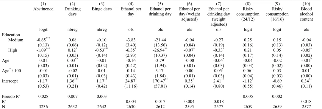
Table A1. Regression models for each indicator of alcohol consumption for females
(1) (2) (3) (4) (5) (6) (7) (8) (9) (10)
Abstinence Drinking
days Binge days Ethanol per
day Ethanol per
drinking day Ethanol per day (weight adjusted)
Ethanol per drinking day
(weight adjusted)
Risky consumption
(24/12)
Risky consumption
(16/16)
Blood alcohol content
logit nbreg nbreg ols ols ols ols logit logit ols
Education
Medium -0.66*** 0.13+ -0.57** 1.16 -5.74+ 0.02 -0.06 0.15 -0.11 -0.01
(0.11) (0.07) (0.20) (0.98) (2.98) (0.01) (0.04) (0.17) (0.20) (0.01)
High -1.07*** 0.41*** -0.79*** 1.84* -11.06*** 0.03** -0.13*** 0.62*** 0.28 -0.02***
(0.13) (0.07) (0.22) (0.74) (2.81) (0.01) (0.04) (0.19) (0.21) (0.01)
Age 0.01 0.01 -0.14*** -0.20 -2.15*** -0.00+ -0.04*** -0.05+ -0.06+ -0.01***
(0.02) (0.01) (0.04) (0.19) (0.42) (0.00) (0.01) (0.03) (0.03) (0.00)
Age2 / 100 -0.02 0.00 0.14** 0.24 2.04*** 0.01+ 0.04*** 0.06+ 0.07+ 0.01***
(0.03) (0.01) (0.05) (0.21) (0.50) (0.00) (0.01) (0.03) (0.04) (0.00)
Intercept -0.43 1.20*** 3.18*** 11.27** 97.01*** 0.21*** 1.63*** -0.76 -0.76 0.27***
(0.37) (0.21) (0.61) (3.92) (9.21) (0.05) (0.13) (0.48) (0.57) (0.02)
Pseudo R2 0.023 0.010 0.013 0.009 0.005
R2 0.002 0.039 0.003 0.051 0.051
N 4213 3016 3020 2995 2976 2954 2935 3041 3041 2935
Notes: Regression models: logit = binary logistic regression; nbreg = negarive binomial regression; ols = ordinary least squares regression.
Unstandardized regression coefficients, standard errors in parentheses. Reference category for education: low education. Predictions in Figures 1, 2, and 3 are based on these 10 models. Significance levels: + .1, * .05, ** .01, *** .001. Source: Epidemiological Survey on Substance Abuse 2012;
weighted results.
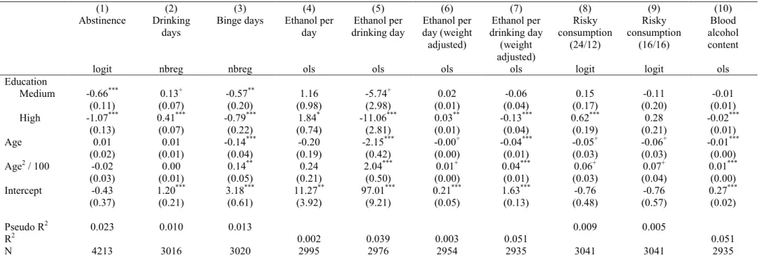
Table A2. Regression models for each indicator of alcohol consumption for males
(1) (2) (3) (4) (5) (6) (7) (8) (9) (10)
Abstinence Drinking
days Binge days Ethanol per
day Ethanol per
drinking day Ethanol per day (weight adjusted)
Ethanol per drinking day
(weight adjusted)
Risky consumption
(24/12)
Risky consumption
(16/16)
Blood alcohol content
logit nbreg nbreg ols ols ols ols logit logit ols
Education
Medium -0.65*** 0.08 -0.10 -3.83 -21.44 -0.04 -0.27 0.25 0.15 -0.04
(0.13) (0.06) (0.12) (3.40) (13.56) (0.04) (0.19) (0.16) (0.13) (0.03)
High -1.09*** 0.12* -0.53*** -6.35* -26.94** -0.07+ -0.33* 0.21 0.05 -0.05*
(0.15) (0.05) (0.14) (2.93) (10.37) (0.04) (0.14) (0.17) (0.14) (0.02)
Age 0.01 0.03** -0.01 -0.16 -3.79+ -0.00 -0.06* -0.04 -0.02 -0.01*
(0.03) (0.01) (0.02) (0.42) (1.94) (0.01) (0.03) (0.03) (0.02) (0.00)
Age2 / 100 -0.01 -0.02 0.01 0.14 3.17+ 0.00 0.05* 0.06+ 0.03 0.01*
(0.03) (0.01) (0.03) (0.43) (1.84) (0.01) (0.03) (0.04) (0.03) (0.00)
Intercept -1.17* 1.36*** 1.17** 24.87* 170.47** 0.35* 2.41** -1.12* -0.69 0.34**
(0.53) (0.21) (0.42) (11.16) (57.01) (0.14) (0.80) (0.55) (0.46) (0.11)
Pseudo R2 0.028 0.007 0.003 0.005 0.002
R2 0.004 0.017 0.004 0.018 0.018
N 3236 2632 2642 2630 2612 2595 2577 2659 2659 2577
Notes: Regression models: logit = binary logistic regression; nbreg = negarive binomial regression; ols = ordinary least squares regression.
Unstandardized regression coefficients, standard errors in parentheses. Reference category for education: low education. Predictions in Figures 1, 2, and 3 are based on these 10 models. Significance levels: + .1, * .05, ** .01, *** .001. Source: Epidemiological Survey on Substance Abuse 2012;
weighted results.