Quantum Fields near Black Holes

Quantum Fields near Black Holes

Andreas Wipf

Theoretisch-Physikalisches Institut Friedrich-Schiller-Universit¨ at Max Wien Platz 1, 07743 Jena

Contents

1 Introduction 1

2 Quantum Fields in Curved Spacetime 2

3 The Unruh Effect 10

4 The Stress-Energy Tensor 15

4.1 Calculating the stress-energy tensor . . . . 18

4.2 Effective actions and h T _µν i in 2 dimensions . . . . 20

4.3 The KMS condition . . . . 25

4.4 Euclidean Black Hole . . . . 26

4.5 Energy-momentum tensor near a black hole . . . . 28

4.6 s-wave contribution to h T µν i . . . . 29

5 Wave equation in Schwarzschild spacetime 31

6 Back-reaction 34

7 Generalisations and Discussion 36

7.1 Hawking radiation of rotating and charged holes . . . . 36 7.2 Loss of Quantum Coherence . . . . 38

1 Introduction

In the theory of quantum fields on curved spacetimes one considers gravity as a classical background and investigates quantum fields propagating on this background. The structure of spacetime is described by a manifold M with metric g _µν . Because of the large difference between the Planck scale (10

cm) and scales relevant for the present standard model ( ≥ 10

cm) the range of validity of this approximation should include a wide variety of interesting phenomena, such as particle creation near a black hole with Schwarzschild radius much greater than the Planck length.

The difficulties in the transition from flat to curved spacetime lie in the absence of the notion of global inertial observers or of Poincare transfor- mations which underlie the concept of particles in Minkowski spacetime. In flat spacetime, Poincare symmetry is used to pick out a preferred irreducible representation of the canonical commutation relations. This is achieved by selecting an invariant vacuum state and hence a particle notion. In a gen- eral curved spacetime there does not appear to be any preferred concept of particles. If one accepts, that quantum field theory on general curved spacetime is a quantum theory of fields, not particles, then the existence of global inertial observers is irrelevant for the formulation of the theory.

For linear fields a satisfactory theory can be constructed. Recently Brunelli and Fredenhagen [1] extended the Epstein-Glaser scheme to curved space- times (generalising an earlier attempt by Bunch [2]) and proved perturbative renormalizability of λφ

.

The framework and structure of Quantum field theory in curved spacetimes

emerged from Parkers analysis of particle creation in the very early universe

[3]. The theory received enormous impetus from Hawkings discovery that

black holes radiate as blackbodies due to particle creation [4]. A compre-

hensive summary of the work can be found in the books [5, 6, 7, 8, 9]

2 Quantum Fields in Curved Spacetime

In a general spacetime no analogue of a ’positive frequency subspace’ is available and as a consequence the states of the quantum field will not possess a physically meaningful particle interpretation. In addition, there are spacetimes, e.g. those with timelike singularities, in which solutions of the wave equation cannot be characterised by their initial values. The conditions of global hyperbolocity of ( M , g _µν ) excludes such ’pathological’

spacetimes and ensures that the field equations have a well posed initial value formulation. Let Σ ⊂ M be a hypersurface whose points cannot be joined by timelike curves. We define the domain of dependence of Σ by D(Σ) = { p ∈ M| every inextendible causal curve through p intersects Σ } . If D(Σ) = M , Σ is called a Cauchy surface for the spacetime and M is globally hyperbolic. If ( M , g _µν ) is globally hyperbolic with Cauchy surface Σ, then M has topology R × Σ. Furthermore, M can be foliated by a one-parameter family of smooth Cauchy surfaces Σ _t , i.e. a smooth ’time coordinate’ t can be chosen on M such that each surface of constant t is a Cauchy surface [10]. In such a spacetime there is a well posed initial value problem for linear wave equations [11]. For example, given smooth initial data φ

, φ ˙

, then there exists a unique solution φ of the Klein-Gordon equation

2 g φ + m

φ = 0, 2 g = 1

√ − g ∂ _µ ( √

− gg ^µν ∂ _ν ). (1) which is smooth on all of M , such that on Σ we have

φ = φ

and n ^µ ∇ µ φ = ˙ φ

,

where n ^µ is the unit future-directed normal to Σ. In addition φ varies continuously with the initial data.

For the phase-space formulation we slice M by spacelike Cauchy surfaces Σ _t and introduce unit normal vector fields n ^µ to Σ _t . The spacetime metric g _µν induces a spatial metric h _µν on each Σ _t by the formula

g _µν = n _µ n _ν − h _µν .

Let t ^µ be a ’time evolution’ vector field on M satisfying t ^µ ∇ µ t = 1. We decompose it into its parts normal and tangential to Σ _t ,

t ^µ = N n ^µ + N ^µ ,

where we have defined the lapse function N and the shift vector N ^µ tangen- tial to the Σ _t . Now we introduce adapted coordinates x ^µ = (t, x ⁱ ), i = 1, 2, 3 with t ^µ ∇ µ x ⁱ = 0, so that t ^µ ∇ µ = ∂ _t and N ^µ ∂ _µ = N ⁱ ∂ _i . The metric coeffi- cients in this coordinate system are

g

= g(∂ _t , ∂ _t ) = N

− N ⁱ N _i and g

= g(∂ _t , ∂ _i ) = − N _i , where N _i = h _ij N ^j , so that

ds

= (N dt)

− h _ij (N ⁱ dt + dx ⁱ )(N ^j dt + dx ^j ) (∂φ)

= 1

N

(∂

φ − N ⁱ ∂ _i φ)

− h ^ij ∂ _i φ∂ _j φ.

The determinant g of the 4-metric is related to the determinant h of the 3-metric as g = − N

h. Inserting these results into the Klein-Gordon action

S = Z

Ldt = 1 2

Z

η g ^µν ∂ _µ φ∂ _ν φ − m

φ

, η = ^q | g | d

x,

one obtains for the momentum density, π, conjugate to the configuration variable φ on Σ _t

π = ∂L

∂ φ ˙ =

√ h

N ( ˙ φ − N ⁱ ∂ _i φ) = √

h(n ^µ ∂ _µ φ).

A point in classical phase space consists of the specification of functions (φ, π) on a Cauchy surface. By the result of Hawking and Ellis, smooth (φ, π) give rise to a unique solution to (1). The space of solutions is independent on the choice of the Cauchy surface.

For two (complex) solutions of the Klein-Gordon equation the inner product (u

, u

) ≡ i

Z

Σ

u ¯

n ^µ ∇ µ u

− (n ^µ ∇ µ u ¯

)u

√

h d

x = i Z

(¯ u

π

− π ¯

u

)d

x

defines a natural symplectic structure. Natural means, that (u

, u

) is inde-

pendent of the choice of Σ. This inner product is not positive definite. Let

us introduce a complete set of conjugate pairs of solutions (u _k , u ¯ _k ) of the Klein-Gordon equation

satisfying the following ortho-normality conditions

(u _k , u _k

) = δ(k, k

) ⇒ (¯ u _k , u ¯ _k

) = − δ(k, k

) and (u _k , u ¯ _k

) = 0.

There will be an infinity of such sets. Now we expand the field operator in terms of these modes:

φ = Z

dµ(k) a _k u _k + a

_k u ¯ _k and π = Z

dµ(k) a _k π _k + a

_k π ¯ _k , so that

(u _k , φ) = a _k and (¯ u _k , φ) = − a

_k .

By using the completeness of the u _k and the canonical commutation relations one can show that the operator-valued coefficients (a _k , a

_k ) satisfy the usual commutation relations

[a _k , a _k

] = [a

_k , a

_k

] = 0 and [a _k , a

_k

] = δ(k, k

). (2) We choose the Hilbert space H to be the Fock space built from a ’vacuum’

state Ω u satisfying

a _k Ω _u = 0 for all k, (Ω _u , Ω _u ) = 1. (3) The ’vectors’ Ω u , a

_k Ω u , . . . comprise a basis of H . The scalar product given by (2,3) is positive-definite.

If (v _p , v ¯ _p ) is a second set of basis functions, we may as well expand the field operator in terms of this set

φ = Z

dµ(p) b _p v _p + b

_p v ¯ _p .

The second set will be linearly related to the first one by v _p =

Z

dµ(k) (u _k , v _p )u _k − (¯ u _k , v _p )¯ u _k ≡ Z

dµ(k) α(p, k)u _k + β(p, k)¯ u _k

¯ v _p =

Z

dµ(k) (u _k , ¯ v _p )u _k − (¯ u _k , v ¯ _p )¯ u _k ≡ Z

dµ(k) β(p, k)u ¯ _k + ¯ α(p, k)¯ u _k .

1

the k are any labels, not necessarily the momentum

The inverse transformation reads u _k =

Z

dµ(p) v _p α(p, k) ¯ − ¯ v _p β(p, k)

¯ u _k =

Z

dµ(p) − v _p β(p, k) + ¯ ¯ v _p α(p, k) . As a consequence the Bogolubov-coefficients are related by

αα

− ββ

= 1 and αβ ^t − βα ^t = 0. (4) If the β(k, p) vanish, then the ’vacuum’ is left unchanged, but if they do not, we have a nontrivial Bogolubov transformation

( a a

) = ( b b

)

α β β ¯ α ¯

and

b b

=

α ¯ − β ¯

− β α a a

. (5)

which mixes the annihilation and creations operators. If one defines a Fock space and a ’vacuum’ corresponding to the first mode expansion,

a _k Ω u = 0,

then the expectation of the number operator b

_p b p defined with respect to the second mode expansion is

(Ω _u , b

_p b _p Ω _u ) = Z

dµ(k) | β(p, k) |

.

That is, the old vacuum contains new particles. It may even contain an infinite number of new particles, in which case the two Fock spaces cannot be related by a unitary transformation.

Stationary and static space-times

A space-time is stationary if there exists a special coordinate system in

which the metric is time-independent. This property holds iff space-time

admits a timelike Killing field K = K ^µ ∂ µ which fulfils the Killing equation

L _K g _µν = 0 ∇ µ K _ν + ∇ ν K _µ = 0. In a static spacetime the timelike Killing

field is everywhere orthogonal to a family of hypersurfaces or satisfies the

Frobenius condition (has vanishing vorticity) ˜ K ∧ d K ˜ = 0, K ˜ = K µ dx ^µ .

Given such a Killing field, we may introduce adapted coordinates along the

congruence and in one hypersurface such that the metric is time-independent

and the shift vector N _i vanishes.

If spacetime is stationary, there is a natural choice for the mode functions u _k : one may introduce a coordinate t upon which the metric does not depend and with respect to which (the globally timelike) K takes the form K = ∂ t . Since ds

= g

dt

+ . . . = (K, K )dt

+ . . ., the coordinate t is in general not the proper time of observers moving with the flow of K. However, since

∇ K (K, K) = 0, we may scale K such that t is the proper time measured by at least one comoving clock. Now we may choose basis functions u _k that satisfy

iL K u _k = ω(k)u _k and iL K u ¯ _k = − ω(k)¯ u _k ,

where the ω(k) > 0 are constant. The ω(k) are the frequencies relative to the particular comoving clock and the u _k and ¯ u _k are the positive and negative frequency solutions, respectively. Now the construction of the vacuum and Fock space is done as described above.

If spacetime is static, we may choose coordinates (t, x ⁱ ) such that K = ∂ t and (g µν ) =

N

0 0 − h _ij

is time-independent. As modes we use u _k = 1

p 2ω(k) e

φ _k (x ⁱ )

which diagonalise L _K . The Klein-Gordon equation simplifies to K φ _k ≡ − N

√ h ∂ _i (N √

hh ^ij ∂ _j ) + N

m

φ _k = ω

_k φ _k . Since n ^µ ∂ _µ = N

∂ _t the inner product of two mode functions is

(u

, u

) = ω

+ ω

2 √

ω

ω

e ^i(ω

Z φ ¯

φ

N

√ h d

x

| {z }

(φ1

,φ

.

The elliptic operator K is symmetric with respect to the L

scalar product (., .)

and may be diagonalised. Its positive eigenvalues are the ω

(k) and its eigenfunctions form a complete ’orthonormal’ set on Σ, (φ _k , φ _k

)

= δ(k, k

).

It follows then that the u _k form a complete set with the properties discussed earlier.

Ashtekar and Magnon [13] and Kay [14] gave a rigorous construction of the

Hilbert-space and Hamiltonian in a stationary spacetime. They started with

a conserved positive scalar product (., .) _E defined by the energy norm. This norm is invariant under the time-translation map

α

_t (φ) = φ ◦ α _t or (α

_t (φ))(x) = φ(α _t (x)),

generated by the Killing field. When completeing the space of complex solutions in the ’energy-norm’ one gets a complex (auxiliary) Hilbertspace H ˜ . The time translation map extends to ˜ H and defines a one-parameter unitary group

α

_t = e ⁱ

^ht , ˜ h self-adjoint.

Note, that from the definition of the Lie derivative, d

dt (α

_t φ) | t=0 = − L K φ = i ˜ hφ.

The conserved inner product (φ

, φ

) can be bounded by the energy norm and hence extends to a quadratic form on ˜ H . Let ˜ H

be the positive spectral subspace of ˜ H and let K be the projection map P : ˜ H → H ˜

. For all real solutions we may now define the scalar product as the inner product of the projected solutions, which are complex. The one-particle Hilbert space H is just the completion of the space ˜ H

of ’positive frequency solutions’ in the Klein-Gordon inner product.

Hadamard states

For a black hole the global Killing field is not everywhere timelike. One may exclude the non-timelike region from space time which corresponds to the imposition of boundary conditions. One may also try to retain this region but attempt to define a meaningful vacuum by invoking physical arguments.

In general spacetimes there is no Killing vector at all. One probably has to give up the particle picture in this generic situation.

In (globally hyperbolic) spacetimes without any symmetry one can still con- struct a well-defined Hilbertspace, namely the Fockspace over a quasifree vacuum state, provided that the two-point functions satisfies the so-called Hadamard condition. Hadamard states are states, for which the two-point function has the following singularity structure

ω(φ(x)φ(y)) ≡ ω

(x, y) = u

σ + v log σ + w, (6)

where σ(x, y) is the square of the geodesic distance of x and y and u, v, w are

smooth functions on M . It has been shown that if ω

has the Hadamard singularity structure in a neighbourhood of a Cauchy-surface, then it has this form everywhere [17]. To show that, one uses that ω

satisfies the wave equation. This result can then be used to show that on a globally hyperbolic spacetime there is a wide class of states whose two-point functions have the Hadamard singularity structure.

The two-point function ω

must be positive, ω(φ(f )

φ(f)) =

Z

dµ(x)dµ(y) ω

(x, y)) ¯ f (x)f (y) ≥ 0,

and must obey the Klein-Gordon equation. These requirements determine u and v uniquely and put stringent conditions on the form of w.

In a globally hyperbolic spacetime the Cauchy problem has a unique solu- tion. It follows that there are unique retarded and advanced Greenfunctions

∆ _ret (x, y) , ∆ _adv (x, y) with supp(∆ _ret ) = { (x, y); x ∈ J

(y) } . The Feynman Greenfunction is related to ω

and the advanced Greenfunc- tion as

i∆ _F (x, y) = ω

(x, y) + ∆ _adv (x, y).

Since ∆ _adv is unique, the ambiguities of ∆ F are the same as those of ω

. The propagator function

i∆(x, y) = [φ(x), φ(y)] = ∆ _ret (x, y) − ∆ _adv (x, y) determines the antisymmetric part of ω

,

ω

(x, y) − ω

(y, x) = i∆(x, y),

so that this part is without ambiguities. For a scalar field without selfinter- action we expect that

ω(φ(x

) . . . φ(x _n )) = 0 for odd n ω(φ(x

) . . . φ(x

)) = ^X

i1<i2...<in j1<j2...<jn

Y n k=1

ω(φ(x _i

)φ(x _j

)).

A state ω fulfilling these conditions is called quasifree. Now one can show

that any choice of ω

(x, y) fulfilling the properties listed above give rise to

a well-defined Fock-space

F = M

n=0

F n , (7)

over a quasifree vacuum state. The scalar-product on the ’n-particle sub- space’ F n in

F n = { ψ ∈ D ( M ⁿ ) _symm / N } ^completion (8) is

(ψ

, ψ

) = Z

dµ(x

, .., x _n , y

, .., y _n ) Y n i=1

ω

(x _i , y _i ) ¯ ψ

(x

, .., x _n )ψ

(y

, .., y _n ), where we introduced the abbreviation dµ(x

, x

, ..) = dµ(x

)dµ(x

) . . .. Since ω

satisfies the wave equation, the functions in the image of 2 + m

have zero norm. The zero-norm states has been divided out in order to end up with a positive definite Hilbertspace.

The smeared field operator is now defined in the usual way:

φ(f ) = a(f )

+ a( ¯ f), where

(a( ¯ f )ψ) _n (x

, .., x _n ) = √ n + 1

Z

dµ(x, y)ω

(x, y)f (x)ψ _n+1 (y, x

, .., x _n ) (a(f )

ψ) _n (x

, .., x _n ) = 1

√ n X n k=1

f (x _k )ψ n−1 (x

, .., x ˇ _k , .., x _n ), n > 0 and (a(f )

ψ)

= 0. It is now easy to see that ω

is just the Wightman function of φ in the vacuum state ψ

:

ω

(x, y) = (ψ

, φ(x)φ(y)ψ

).

3 The Unruh Effect

We may ask the question how quantum fluctuations appear to an accelerat-

ing observer? In particular, if the observer were carrying with him a robust

detector, what would this detector register? If the motion of the observer

undergoing constant (proper) acceleration is confined to the x

axis, then the world line is a hyperbola in the x

, x

plane with asymptotics x

= ± x

. These asymptotics are event horizons for the accelerated observer. It is helpful to use a noninertial frame of reference attached to the observer. To find this frame we consider a family of accelerating observers, one for each hyperbola with asymptotics x

= ± x

. The natural coordinate system is then the comoving one in which along each hyperbola the space coordinate is constant while the time coordinate τ is proportional to the proper time as measured from an initial instant x

= 0 in some inertial frame. The world lines of the uniformly accelerated particles are the orbits of one-parameter group of Lorentz boost isometries in the 3-direction:

x

x

= ρ

sinh κt cosh κt

= e ^κωt 0

ρ

, (ω ^µ _ν ) = 0 1

1 0

. In the comoving coordinates (t, ρ, x

, x

)

ds

= κ

ρ

dt

− dρ

− (dx

)

− (dx

)

.

so that the proper time along a hyperbola ρ =const is κρt. The orbits are tangential to the Killing field

K = ∂ t = κ(x

∂

+ x

∂

) with (K, K) = (κρ)

= g

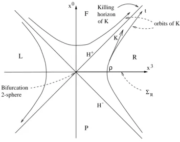
. (9) Some typical orbits are depicted in figure (1). Since the proper acceleration on the orbit with (K, K) = 1 or ρ = 1/κ is κ, it is conventional to view the orbits of K as corresponding to a family of observers associated with an observer who accelerates uniformly with acceleration a = κ.

The coordinate system t, ρ covers the Rindler wedge R on which K is timelike future directed. The boundary H

and H

of the Rindler wedge is given by ρ = 0 and appears as a Killing horizon, on which K becomes null. Beyond this event horizon the Killing vector field becomes spacelike in the regions F, P and timelike past directed in L. The parameter κ plays the role of the surface gravity. To see that, we set r − 2M = ρ

/8M in the Schwarzschild solution and linearise the metric near the horizon r ∼ 2M . One finds that

ds

∼ (κρ)

dt

− dρ

| {z }

2-dim Rindler spacetime

− 1 4κ

dΩ

| {z }

2-sphere of radius 1/2κ

contains the line element of 2-dimensional Rindler spacetime, where κ =

1/4M is indeed the surface gravity of the Schwarzschild black hole.

F

P L R

K x

x

ρ

H

Killing horizon

Bifurcation 2-sphere

orbits of K of K

t

H

Σ

Figure 1: A Rindler-observer sees only a quarter of Minkowski space Killing horizons and surface gravity

The notion of Killing horizons is relevant for the Hawking radiation and the thermodynamics of black holes and can already be illustrated in Rindler spacetime. Let S(x) be a smooth function and consider a family of hyper- surfaces S(x) = const. The vector fields normal to the hypersurfaces are

l = g(x)(∂ ^µ S)∂ _µ ,

with arbitrary non-zero function g. If l is null, l

= 0, for a particular hyper- surface N in the family, N is said to be a null hypersurface. For example, the normal vectors to the surfaces S = r − 2M = const in Schwarzschild spacetime have norm

l

= g

g ^µν ∂ µ S∂ ν S = g

1 − 2M r

,

so the horizon at r = 2M is a null hypersurface.

Let N be a null hypersurface with normal l. A vector t tangent to N is characterised by (t, l) = 0. But since l

= 0, the vector l is itself a tangent vector, i.e.

l ^µ = dx ^µ

dλ , where x ^µ (λ) is a null curve on N .

Now one can show, that ∇ l l ^µ |

∼ l ^µ , which means that x ^µ (λ) is a geodesic with tangent l. The function g can be chosen such that ∇ l l = 0, i.e. so that λ is an affine parameter. A null hypersurface N is a Killing horizon of a Killing field K if K is normal to N .

Let l be normal to N such that ∇ l l = 0. Then, since on the Killing horizon K = f l for some function f , it follows that

∇ K K ^µ = f l ^ν ∇ ν (f l ^µ ) = f l ^µ l ^ν ∂ _ν f = ( ∇ K log | f | )K ^µ ≡ κK ^µ on N . One can show, that the surface gravity κ =

∇ K log f

is constant on orbits of K. If κ 6 = 0, then N is a bifurcate Killing horizon of K with bifurcation 2-sphere B. In this non-degenerate case κ

is constant on N . If N is a Killing horizon of K with surface gravity κ, then it is also a Killing horizon of cK with surface gravity c

κ. Thus the surface gravity depends on the normalisation of K. For asymptotically flat spacetimes there is the natural normalisation K

→ 1 and future directed as r → ∞ . With this normal- isation the surface gravity is the acceleration of a static particle near the horizon as measured at spatial infinity.

A Killing field is uniquely determined by its value and the value of its deriva- tive F µν = ∇

K _ν] at any point p ∈ M. At the bifurcation point p of a bifurcate Killing horizon K vanishes, K(p) = 0, and hence is determined by F _µν (p). In 2 dimensions F _µν (p) is unique up to scaling. The infinitesimal action of the isometries α t generated by K takes a vector v ^µ at p into

L _K v ^µ = F ^µ _ν v ^ν . (10)

The nature of the map on T _p depends upon the signature of the metric. For Riemannian signature it is an infinitesimal rotation and the orbits of α _t are closed with a certain period. For Lorentz signature (10) is an infinitesimal Lorentz boost and the orbits of α _t have the same structure as in the Rindler case. A similar analysis applies to higher dimensions.

For example, for the Killing field (9) we have

∇ K K = ± κK = ⇒ surface gravity = ± κ.

The Rindler wedge R is globally hyperbolic with possible Cauchy hyper-

surface Σ _R . Thus it may be viewed as spacetime in its own right and we

may construct a quantum field theory on it. When we do that, we obtain

a remarkable conclusion, namely that the standard Minkowski vacuum Ω _M corresponds to a thermal state in the new construction. This means, that an accelerated observer will feel himself to be immersed in a thermal bath of particles with temperature proportional to his acceleration a [15],

kT = ¯ ha/2πc.

Unruh pointed out in addition that a Rindler detector would detect these particles. The noise along a hyperbola is greater than the noise along a geodesic, and this excess noise excites the Rindler detector. A uniformly accelerated detector in its ground state may jump spontaneously to an ex- cited state. Note that the temperature tends to zero in the limit in which Planck’s constant h tends to zero. Such a radiation has non-zero entropy.

Since the use of a accelerated frame seems to be unrelated to any statistical average, the appearance of a non-vanishing entropy is rather puzzling.

The Unruh effect shows, that at the quantum level there is deep relation between the theory of relativity and the theory of fluctuations associated with states of thermal equilibrium, two major aspects of Einstein’s work:

The distinction between quantum zero-point and thermal fluctuations is not an invariant one, but depends on the motion of the observer.

Note that the temperature is proportional to the acceleration a of the ob- server. Since a = 1/ρ this means that T ρ = const ⇐⇒ T √ g

= const. This is just the Tolman-Ehrenfest relation [18] for the temperature in a fluid in hydrostatic equilibrium in a gravitational field. The factor √ g

guarantees that no work can be gained by transferring radiation between two regions at different gravitational potentials.

Let us calculate the number of ’Rindler-particles’ in Minkowski vacuum. To simplify the analysis, we consider a zero-mass scalar field φ in 2-dimensional Minkowski space. In the Heisenberg picture, the expansions in terms of annihilation and creation operators are

φ = Z

dk a _k u _k + h.c. , where u _k = 1

√ 4πω e

, ω = | k | and

φ = Z

dp b _p v _p + h.c. , where v _p = 1

√ 4π ρ ^ip/κ e

, = | p | .

The β-coefficients are found to be β(p, k) = − (¯ u _k , v _p ) = 1

4π Z

0

r ω −

r ω

1 κρ

e ^ikρ ρ ^ip dρ,

where we have evaluated the time-independent ’scalar-product’ at t = 0 for which x

= 0. Using the formula

Z

0

dx x ^ν−1 e

= Γ(ν)(α

+ β

)

e

we arrive at

β(p, k) = − Γ(ip/κ)

4πκ ω

^r ω ± p

√ ω

e

for k ω = ± 1, or at

| β(p, k) |

= 1 2πκω

1 e

− 1 .

The Minkowski spacetime vacuum is characterised by a _k Ω _M = 0 for all k.

Assuming that this is the state of the system, the expectation value of the occupation number as defined by the Rindler observer, n _p ≡ b

_p b _p , is found to be

(Ω _M , n _p Ω _M ) = Z

dk | β(p, k) |

= volume × 1

e

− 1 , (11) Thus for an accelerated observer the quantum field seems to be in an equi- librium state with temperature proportional to T = κ/2π = a/2π. Note, that in cgs units, this becomes

(T /1 ^o K) = (a/10

cm/sec

). (12) Since T tends to zero as ρ → ∞ the Hawking temperature (i.e. temperature as measured at spatial ∞ ) is actually zero. This is expected since there is nothing inside which could radiate. But for a black hole T _local → T H at infinity and the black hole must radiate at this temperature.

Let us finally see, how the (massless) Feynman-Greenfunction in Minkowski spacetime,

i∆ _F (x, x

) = h 0 | T(φ(x)φ(x

)) | 0 i = i 4π

1

(x − x

)

− i ,

appears to an accelerated observer. Let x = (t, ρ) and x

= (t

, ρ) be two events on the worldline of an accelerated observer. Since the invariant dis- tance of these two events is 2ρ sinh ^κ

(t − t

), we have

∆ F (x, x

) = i 16π

ρ

1

sinh

^κ

(t − t

) − i . (13) After a Fourier transformation one arrives at the following spectral repre- sentation of the Feynman-propagator as seen by this observer

∆ _F (x, x

) = 1 (2π)

( κ

ρ )

Z

d

p e

1

p

+ i − 2πi δ(p

) e ^β|E| − 1

. (14) This is the finite temperature propagator. It follows, that, in equilibrium, atoms dragged along the world line find their excited levels populated as predicted by a temperature β

= a/2π.

4 The Stress-Energy Tensor

The operator of primary interest is the energy-momentum tensor. It de- scribes the local energy, momentum and stress properties of the field and is relevant for studying the back-reaction of the quantum field on the spacetime geometry. Semiclassically one would expect that back-reaction is described by the ’semiclassical Einstein equation’

G _µν = 8πG h T _µν i ,

where the right-hand side contains the expectation value of the energy- momentum tensor of the relevant quantised field in the chosen state. If the characteristic curvature radius L in a region of spacetime is much greater then the Planck length l _pl = ^p ¯ hG/c

, then in the calculation of h T _µν i one can expand in the small parameter = (l _pl /L)

and retain only the terms up to first order in (one-loop approximation). The term of order , containing a factor ¯ h, represents the main quantum correction to the classical result.

In the one-loop approximation the contributions of all fields to h T _µν i are additive and thus can be studied independently.

Some restrictions should be expected on the class of states on which h T _µν i

can be defined. The Hadamard condition provides a restriction of exactly this sort of states.

The difficulties with defining

h T _µν i = ω(T _µν )

are present already in Minkowski spacetime. The divergences are due to the vacuum zero-fluctuations. The methods of extracting a finite, physically meaningful part, known as renormalisation procedures, were extensively dis- cussed in the literature [20]. A simple cure for this difficulty is (for free fields) the normal ordering prescription:

ω( : T _µν : ) = ω(T _νν ) − (Ω _M , T _µν Ω _M ).

The so defined vacuum expectation value of the stress-energy tensor van- ishes. On curved spacetime there is no satisfactory generalisation of this prescription since there is there is no preferred vacuum state and due to vacuum polarisation effects we do not expect that the stress-energy of the vacuum (assuming there is a natural one) vanishes.

To make progress let us look at an alternative formulation of the normal ordering prescription. We first consider the ill-defined object φ

(x), which is part of the stress-energy tensor. We may split the points and consider first the object ω(φ(x)φ(y)) which solves the Klein-Gordon equation. This bi- distribution makes perfectly good sense. For physically reasonable states ω in the Fock space (e.g. states with a finite number of particles) the singular behaviour of this bi-distribution is the same as that belonging to the vacuum state, ω

(φ(x)φ(y)). For such states the difference

F (x, y) = ω(φ(x)φ(y)) − ω

(φ(x)φ(y))

is a smooth function of its arguments. Hence, after performing this ’vacuum subtraction’ the coincidence limit may be taken. We then define

ω(φ

(x)) = lim

x→y F (x, y).

The same prescription can be used for the stress-energy tensor instead of φ

. We define

ω(T µν (x)) = lim

x→x

D _µν

F (x, x

), D _µν

= ∂ µ ∂ _ν

− 1

2 g µν [∂ α ∂ ^α

− m

] .

Although this is not a physical definition of expectation values of the stress- energy tensor it sensibly defines the differences of the expected stress energy between two states,

ω

(T _µν ) − ω

(T _µν ).

In the absence of an obvious prescription to define the expectation values, it is useful to take an axiomatic approach. Wald showed that a renormalised stress tensor satisfying certain reasonable physical requirements is essentially unique [19]. Its ambiguity can be absorbed into redefinitions of the coupling constants in the (generalised) gravitational field equation. Wald argues that one expects this operator to have the following properties:

1. Consistency: Whenever ω

(φ(x)φ(y)) − ω

(φ(x)φ(y)) is a smooth function, then ω

(T _µν ) − ω

(T _µν ) is well-defined and should be given by the above ’point-splitting’ prescription.

2. Conservation: In the classical theory the stress-energy tensor is con- served. If the regularisation needed to define a stress-energy tensor respects the diffeomorphism invariance, then

∇ ν T ^µν = 0

must also hold in the quantised theory. This property is needed for consistency of Einstein’s gravitational field equation.

3. In Minkowski spacetime, we have (Ω _M , T _µν Ω _M ) = 0.

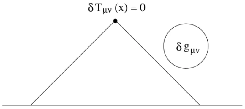
4. Causality: We assume, that spacetime is asymptotically static. For a fixed in-state, ω _in (T _µν (x)) is independent of variations of g _µν outside the past lightcone of x. For a fixed out-state, ω out (T µν ) is independent of metric variations outside the future light cone of x.

The first and last properties are the key ones, since they uniquely determine the expected stress-energy tensor up to the addition of local curvature terms.

This fact is contained in the

Uniqueness theorem (Wald): Let T _µν and ˜ T _µν be operators on globally hyperbolic spacetime satisfying the axioms of Wald. Then the difference

U _µν = T _µν − T ˜ _µν

fixed initial geometry and state

µν (x) = 0

g µν

δ δ T

Figure 2: Changes outside the past lightcone do not affect h T _µν (x) i . 1. is a multiple of the identity operator,

2. is conserved, ∇ ν U ^µν = 0,

3. is a local tensor of the metric. That is, it depends only on the metric and its derivatives, via the curvature tensor, at the same point x.

As a consequence of the properties,

ω(T _µν ) − ω( ˜ T _µν )

is independent on the state ω and depends only locally on curvature invari- ants. The Causality axiom can be replaced by a locality property, which does not assume an asymptotically static spacetime. The proofs of these properties are rather simple and can be found in the standard textbooks.

4.1 Calculating the stress-energy tensor

A ’point-splitting’ prescription where one subtracts from ω(φ(x)φ(y)) the expectation value ω

(φ(x)φ(y)) in some fixed state ω

fulfils the consistency requirement, but cannot fulfil the first and third axiom at the same time.

However, if one subtracts a locally constructed bi-distribution H(x, y) which

satisfies the wave equation, has a suitable singularity structure and is equals

to (Ω M , φ(x)φ(y)Ω M ) in Minkowski spacetime, then all four properties will

be satisfied.

To find a suitable bi-distribution one recalls the singularity structure (6) of ω

(x, y). In Minkowski spacetime and for massless fields w = 0 and this suggests that we take the bi-distribution

H(x, y) = u(x, y)

σ + v(x, y) log σ

The resulting stress-energy obeys almost all properties, besides that for mas- sive fields on Minkowski spacetime we still find a non-vanishing vacuum expectation value, and that

∇ ν ω(T ^µν ) = ∇ ν Q,

where Q is a scalar density, locally dependent on the metric. Hence we may modify our prescription by simply subtracting (Q + c)g _µν from T _µν . The constant c is chosen, such that on Minkowski spacetime the vacuum expectation value vanishes.

Effective action

The classical metric energy momentum tensor T _µν (x) = 2

p | g | δS δg ^µν (x)

is symmetric and automatically conserved (for solutions of the field equation) if it is gotten by variation of a diffeomorphism-invariant classical action S. If we could construct a diffeomorphism-invariant quantum or effective action Γ, whose variation with respect to the metric yields an expectation value of the energy momentum tensor,

h T _µν (x) i = 2 p | g |

δΓ δg ^µν (x) ,

then h T _µν i would be conserved by construction. There exists a number of procedures for regularising h T _µν i , i.e. dimensional, point-splitting or zeta- function regularisation, to mention the most popular ones. Some of them are rigorously defined only on Riemannian manifolds. Point-splitting is an ex- ception in this respect. Unfortunately the ’divergent’ part’ of T _µν cannot be completely absorbed into the parameters already present in the theory, i.e.

gravitational and cosmological constant and parameters of the field theory

under investigation. One finds that one must introduce new, dimensionless

parameters.

The regularisation and renormalisation of the effective action is more trans- parent, since it is a scalar. The divergent geometric parts of the effective action, Γ = ^R ηγ _div + Γ _{f inite} have the form

γ _div = A + BR + C(Weyl)

+ D[(Ricci)

− R

] + E ∇

R + F R

.

The part containing A and B can be absorbed into the classical action of gravity. The remaining terms with dimensionless parameters C − F cannot be absorbed into parameters already present in the theory. Upon varia- tion with respect the metric, they lead to a 2-parameter ambiguity in the expression for T _µν .

4.2 Effective actions and h T _µν i in 2 dimensions

In two dimensions there are less divergent terms in the effective action. They have the form

L div = A + BR.

The last topological term does not contribute to T _µν and the first one leads to an ambiguous term ∼ Ag _µν in the energy momentum tensor.

The symmetric stress-energy tensor has 3 components, two of which are (almost) determined by T ^µν

= 0. As independent components we choose the trace T = T ^µ _µ which is a scalar of dimension L

.

The ambiguities in the reconstruction of T ^µν from its trace is most trans- parent if we choose isothermal coordinates (x

, x

)

ds

= e

(dx

)

− (dx

)

)

which always exist in 2-dimensions. Introducing null-coordinates u = 1

2 (x

− x

) and v = 1

2 (x

+ x

) ⇒ ds

= 4e

dudv

the non-vanishing Christoffel symbols are Γ ^u _uu = 2∂ _u σ, Γ ^v _vv = 2∂ _v σ and the Ricci scalar reads R = − 2e

∂ _u ∂ _v σ. Rewriting the conservation in null-coordinates we obtain

∂ _u h T _vv i + e

∂ _v h T i = 0 , ∂ _v h T _uu i + e

∂ _u h T i = 0, (15)

where T = T ^µ _µ = e

T _uv . This shows, that the trace h T i determines h T _vv i

up to a function t _v (v) and h T _uu i up to a function t _u (u). These free functions contain information about the state of the quantum system.

In the case of a classical conformally invariant field, ^class T ^µ _µ = 0. An impor- tant feature of h T _µν i is that its trace does not vanish any more. This trace- anomaly is a state-independent local scalar of dimension L

and hence must be proportional to the Ricci scalar,

h T i = c

24π R = − c

12π e

∂ u ∂ v σ

where c is the central charge of the scale invariant quantum theory. Inserting this trace anomaly into (15) leads to

h T _uu,vv i = − c

12π e ^σ ∂ _u,v

e

+ t _u,v , h T _uv i = − c

12π 2

σ. (16) Formally, the expectation value of the stress-energy tensor is given by the path integral

h T _µν (x) i = − 1 Z[g]

Z

D φ 2

√ g δ

δg ^µν e

= 2

√ g δ δg ^µν Γ[φ], where the effective action is given by

Γ[g] = − log Z[g] = − log Z

D φ e

= 1

2 log det( −4 c )

and we made the transition to Euclidean spacetime (which is allowed for the 2d models under investigation). For arbitrary spacetimes the spectrum of 4 c is not known. However, the variation of Γ with respect to σ in

g _µν = e

ˆ g _µν ,

is proportional to the expectation value of the trace of the stress-energy tensor,

δΓ

δσ(x) = − 2g ^µν (x) δΓ

δg ^µν (x) = − √

g h T ^µ _µ (x) i

and can be calculated for conformally coupled particles in conformally flat spacetimes. From the conformal anomaly one can (almost) reconstruct the effective action.

In particular, in 2 dimensions the result is the Polyakov effective action Γ[g] − Γ[δ] = c

96π

Z √ gR 1

4 R,

where the central charge c is 1 for uncharged scalars and Dirac fermions (see [21] for modifications of this result, for a spacetime with nontrivial topology). The h T µν i is gotten by differentiation with respect to the metric.

The covariant expression is

h T _µν i = c 24π

g _µν R − ∇ µ ∇ ν

1 4 R

+ c

48π ∇ µ

1 4 R · ∇ ν

1 4 R − 1

2 g _µν ∇ ^α 1

4 R · ∇ α

1 4 R ,

(17)

and in isothermal coordinates it simplifies to (16), as it must be. This energy- momentum tensor is consistent, conserved and causality restricts the choice of the Greenfunction 1/ 4 . The ambiguities in inverting the wave operator in (17) shows up in the free functions t u,v . A choice of these functions is equivalent to the choice of the quantum state.

Let us now apply these results to the (t, r) part of the Schwarzschild black hole

ds

= 1 − 2M r

dt

− 1

1 −

_r dr

,

which we treat as 2-dimensional black hole

. We use the ’Regge-Wheeler tortoise coordinate’ r

r

= r + 2M log ( r

M − 2) (18)

such that the metric becomes conformally flat

ds

= 1 − 2M r

(dt

− dr

) ≡ α(dt

− dr

). (19) The event horizon at r = 2M has tortoise coordinate r

= −∞ . As above we introduce null-coordinates u =

(t − r

) and v =

(t + r

). Using

∂ _v = ∂ _t + ∂ _r

and ∂ _r

= α∂ _r we obtain for the light-cone components (16) of the energy momentum tensor

h T _uu,vv i = − c 12π

2M α r

+ M

r

+ t _u,v , h T _uv i = − c 12π

2M α r

2

The resulting energy momentum tensor is not identical to tensor one gets when one

quantises only the s -modes in the 4-dimensional Schwarzschild metric [22].

or for h T _µν i in the x ^µ = (t, r

) coordinate system

h T _µ ^ν i = − cM 24πr

4r + ^M _α 0 0 − ^M _α

+ 1

4α

t _u + t _v t _u − t _v t _v − t _u − t _u − t _v

(20) The state-dependence resides in the free functions t _u,v .

The Boulware state is the state appropriate to a vacuum around a static star and contains no radiation at spatial infinity J

. Hence t _u and t _v must vanish and the energy-momentum of a quantum field around a static star is

h O _s | T _µ ^ν | O _s i = − cM 24πr

4r + ^M _α 0 0 − ^M _α

. (21)

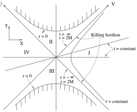
However, this state is singular at the horizon. To see that, we use Kruskal coordinates which are regular at the event horizon :

U = − e

and V = e ^v/2M so that ds

= 16M

r e

dU dV.

With respect to these coordinates the energy momentum tensor takes the form

h T _{U U} i = M U

4t _u − c 3π [ 2M α

r

+ M

r

] h T _{V V} i = M

V

4t _v − c 3π [ 2M α

r

+ M

r

] h T _{U V} i = M

U V c 3π

2M α r

.

For the Boulware vacuum t _u = t _v = 0 and the expectation value the stress- energy momentum is singular at the past and future horizon. The compo- nent h T U U i is regular at the horizon U = 0 if M

t u = c/192π and h T V V i is regular at the horizon V = 0, if M

t _v = c/192π holds. The corresponding state is called the Israel-Hartle-Hawking state. In this state the asymptotic form of the energy-momentum tensor is

h 0 HH | T ^µ _ν | 0 HH i ∼ c 384πM

1 0 0 − 1

= cπ 6 (kT )

1 0 0 − 1

(22)

with T = 1/8πkM = κ/2πk. This is the stress-tensor of a bath of thermal

r = constant t = constant t =

r = 2M IV I

II

III T

X r = 2M 8

t = − 8 r = 0

r = 0 Killing horihon

V U

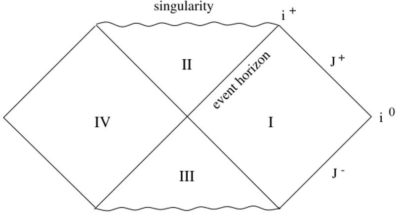
Figure 3: The Kruskal extension of Schwarzschild spacetime radiation at temperature T . Finally, demanding that energy-momentum is regular at the future horizon and that there is no incoming radiation, i.e.

t _u = c

192πM

and t _v = 0 results in

h 0 _U | T ^µ _ν | 0 _U i ∼ c 768πM

1 1

− 1 − 1

= cπ 12 (kT )

1 1

− 1 − 1

(23)

The Unruh state is regular on the future horizon and singular at the past

horizon. It describes the Hawking evaporation process with only outward

flux of thermal radiation.

4.3 The KMS condition

The most elegant and powerful derivation of the Hawking radiation involves an adaption of the techniques due to Kubo to show that the Feynman prop- agator for a space-time with stationary black hole satisfies the KMS con- dition (periodicity of the finite temperature Green function in imaginary time). Consider a system with time-independent Hamiltonian H. The time evolution of an observable in the Heisenberg picture is

A(z) = e ^izH Ae

,

where z = t + iτ is complex time. For τ = 0 it is the time-evolution in a static spacetime with Lorentzian signature and for t = 0 the time- evolution in the corresponding static spacetime with Euclidean signature.

If exp( − βH), β > 0 is trace class, one can define the equilibrium state of temperature T = 1/β :

h A i β = 1

Z tr e

A, Z = tr e

. (24) For two observables A and B we define the thermal expectation values

G ^β

(z, A, B) = h A(z

)B (z

) i β = 1

Z tr e ^i(z+iβ)H Ae

B (25) and

G ^β

(z, A, B) = h B(z

)A(z

) i β = 1

Z tr Be ^izH Ae

(26) where z = z

− z

and we have used the cyclicity under the trace. Both expo- nents in (25) have negative real parts if − β < τ < 0; for (26) the condition reads 0 < τ < β. Therefore, these two formulas define holomorphic func- tions in those respective strips with boundary values G ^β

(t, A, B). From (25,26) it follows immediately, that

G ^β

(z, A, B) = G ^β

(z − iβ, A, B) (27)

For z = t this reads h BA(t) i β = h A(t − iβ)B i β . Condition (27) is called the

KMS condition after Kubo, Martin and Schwinger [23]. It can be given a

precise sense in terms of C

algebras and their states for systems for which exp( − βH) is not trace-class. The KMS-condition is now accepted as a def- inition of ’thermal equilibrium at temperature 1/β’.

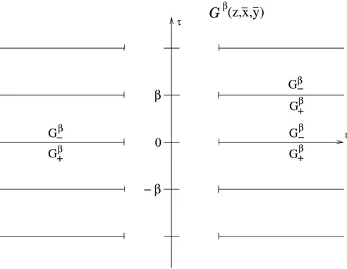
So far the analytic functions G

have been defined in disjoint, adjacent strips in the complex time plane. The KMS-condition states that one of these is the translate of the other and this allows us to define a periodic function throughout the complex plane, with the possible exception of the lines τ = = (z) = nβ. Let A = φ(~x) and B = φ(~y). Because of locality φ(x) and φ(y) commute for spacelike separated events and

[φ(t, ~x), φ(0, ~y)] = 0 for t ∈ I ⊂ R.

Then the boundary values of

G ^β

(z, ~x, ~y) = h φ(z, ~x)φ(0, ~y ) i β and G ^β

(z, ~x, ~y) = h φ(0, ~y)φ(z, ~x) i β

coincide on I and we conclude (by the edge-of-the-wedge theorem) that they are restrictions of a single holomorphic, periodic function, G ^β (z, ~x, ~y), defined in a connected region in the complex time plane except parts of the lines τ = nβ.

4.4 Euclidean Black Hole

The most general spherically symmetric vacuum solution of Einsteins field equation is given by the well-known Schwarzschild line element

ds

= αdt

− 1

α dr

− r

dΩ

, α = 1 − 2M/r. (28) This metric can be analytically extended to

ds

= αdz

− 1

α dr

− r

dΩ

,

with z = t + iτ. Now we perform the same coordinate transformation to (complex) Kruskal coordinates as we did for the Lorentzian solution:

Z = 2e ^r

^/4M sinh z

4M and X = 2e ^r

^/4M cosh z 4M . The line element reads

ds

= 16M

r e

dZ

− dX

− r

dΩ

− β 0 β G

G G G G

β

β β τ

t β (z,x,y)

G

G ^β

− +

− β + ^β +

−

Figure 4: The analycity region of G ^β (z, ~x, ~y).

and the Killing field takes the form K = ∂ z = 1

4M

Z∂ X + X∂ Z

.

The null-hypersurface N = { U = 0 } ∪ { V = 0 } has normal (with affine parametrisation)

l =

∂ _V on { U=0 }

∂ _U on { V=0 } . The surface gravity is

κ = K log | f | = 1

4M V ∂ V log | V | = 1

4M on { U = 0 } κ = K log | f | = − 1

4M U ∂ _U log | U | = − 1

4M on { V = 0 } Let us set Z = T + i T . The orbits of K are

T X

= 2e ^r

^/4M

sinh t/4M cosh t/4M

and

T X

= 2e ^r

^/4M

sin τ /4M cos τ /4M

,

in the Lorentzian and Euclidean slices, respectively. As expected from the general properties of bifurcation spheres, these are Lorentz-boosts and ro- tations, respectively. Since the Euclidean slice is periodic in τ and since the Greenfunction is analytic in z = t + iτ we conclude, that it is peri- odic in imaginary time with period 8πM , G (z, . . .) = G (z + 8πiM, . . .). This corresponds to a temperature T = 1/8πM, the Hawking temperature.

4.5 Energy-momentum tensor near a black hole

In any vacuum spacetime R _µν vanishes and so do the two local curvature terms which enter the formula for T _µν with undetermined coefficients. Hence T _µν is well-defined in the Schwarzschild spacetime. The symmetry of h T ^µ _ν i due to the SO(3) symmetry of the spacetime of a non-rotating black hole and the conservation ∇ ν h T ^µν i reduce the number of independent components of h T ^µ _ν i . Christensen and Fulling [24] showed that in the coordinates (t, r

, θ, φ) the tensor is block diagonal. The (t, r

) part admits the representation

h T ^µ _ν i = T

2

− ^H _αr

− 2Θ 0 0 ^H _αr

+ W

4παr

1 − 1 1 − 1

+ N

αr

− 1 0

0 1

(29) whereas the (θ, φ)-part has the form

h T ^µ _ν i = ( T 4 + Θ)

1 0 0 1

. (30)

Here N and W are two constants and α(r) = 1 − 2M

r

, T (r) = h T ^µ _µ i , Θ(r) = h T ^θ _θ i − 1 4 T (r) H(r) = 1

2 Z r

2M

(r

− M )T (r

)dr

, G(r) = 2 Z r

2M

(r

− 3M)Θ(r

)dr

. The energy-momentum tensor is characterised unambiguously by fixing two functions T (r), Θ(r) and two constants N, W . The constant W gives the intensity of radiation of the black hole at infinity and N vanishes if the state is regular on the future horizon.

The radiation intensity W in non-vanishing only in the Unruh vacuum. The

coefficient W for the massless scalar field (s = 0), two-components neutrino

field (s = 1/2), electromagnetic field (s = 1) and gravitational field (s = 2) have been calculated by Page and Elster [25]:

M

W

M

W

M

W

M

W

7.4 · 10

8.2 · 10

3.3 · 10

0.4 · 10

The coefficient N vanishes for the Unruh and Israel-Hartle-Hawking vacua.

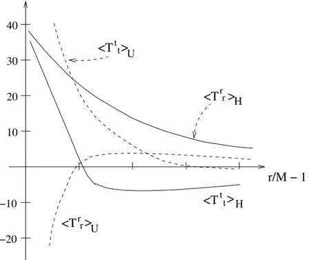
The calculation of the functions in (29,30) meets technical difficulties con- nected with the fact that solutions of the radial mode equation (see be- low) are not expressed through known transcendental functions and, conse- quently, one needs to carry out renormalisation in divergent integrals within the framework of numerical methods. The results for h T ^t _t i and h T ^r _r i for the Israel-Hartle-Hawking and the Unruh states are sketched in the following figure. These calculations have been done by Howard/Candelas and Elster [26]

In the Hartle-Hawking state the Kruskal coordinate components of h T _µν i near the horizon are found to be of order 1/M

. The energy flux into the black hole is negative, as it must be since the ’Hartle-Hawking vacuum’ is time independent and the energy flux at future infinity is positive. This is possible since h T _µν i need not satisfy the energy conditions.

4.6 s -wave contribution to h T _µν i

The covariant perturbation theory for the 4d effective action Γ as developed in [29] is very involved for concrete calculations. Here we shall simplify the problem by considering s-modes of a minimally coupled massless scalar field propagating in an arbitrary (possibly time-dependent) spherically symmetric 4-dimensional spacetime. The easiest way to perform this task is to compute the contribution of these modes to the effective action. We choose adapted coordinates for which the Euclidean metric takes the form

ds

= γ _ab (x ^a ) dx ^a dx ^b + Ω

(x ^a )ω _ij dx ⁱ dx ^j ,

where the last term is the metric on S

. Now one can expand the (scalar) matter field into spherical harmonics. For s-waves, φ = φ(x ^a ), the action for the coupled gravitational and scalar field is

S = − 1 4

Z

[Ω

^γ R + ^ω R + 2( ∇ Ω)

] √ γd

x + 2π Z

Ω

( ∇ φ)

√ γd

x,

40 30 20 10

−10

−20

<T

<T

<T

t t

r r

r r

>

>

> _U

U

H

r/M − 1

<T t t > _H

Figure 5: The dependence of h T ^t _t i and h T ^r _r i (in units of π

T _H

/90) on the distance from the horizon.

where ^γ R is the scalar curvature of the 2d space metric γ _ab , ^ω R = 2 is the scalar curvature of S

and ( ∇ Ω)

= γ ^ab ∂ _a Ω∂ _b Ω. The purely gravitational part of the action is almost the action belonging to 2d dilatonic gravity with two exceptions: first, the numerical coefficient in front of ( ∇ Ω)

is different and second, the action is not invariant under Weyl transformation due to the

ω R term. The action is quite different from the actions usually considered in 2d (string-inspired) field theories, because of the unusual coupling of φ to the dilaton field Ω. Choosing isothermal coordinates, γ _ab = e

γ _ab ^f , where γ _ab ^f is the metric of the flat 2d space, one arrives with ζ-function methods at the following exact result for the effective action for the s-modes [30]

Γ _s =

Γ _s +

Γ

(n)

Γ[σ, Ω] = 1 8π

Z 1 12

γ R 1 4 γ

γ R − 4 γ Ω Ω

1 4 γ

γ R √ γd

x

(i)

Γ[Ω] = Γ _s [σ = 0, Ω] = 1

2 log det − 4 f + 4 f Ω Ω

.