Forecasting IT Security Vulnerabilities - An Empirical Analysis
Emrah Yasasin a∗ , Julian Prester b , Gerit Wagner a , Guido Schryen c
a
Department of Management Information Systems, University of Regensburg, Universit¨ atsstraße 31, 93053 Regensburg, Germany
b
School of Information Systems, UNSW Business School, Kensington NSW 2052, Australia
c
Faculty of Business Administration and Economics, Paderborn University, Warburger Strasse 100, 33098 Paderborn, Germany
Abstract
Today, organizations must deal with a plethora of IT security threats and to ensure smooth and uninterrupted business operations, firms are challenged to predict the volume of IT security vulner- abilities and allocate resources for fixing them. This challenge requires decision makers to assess which system or software packages are prone to vulnerabilities, how many post-release vulnerabili- ties can be expected to occur during a certain period of time, and what impact exploits might have.
Substantial research has been dedicated to techniques that analyze source code and detect security vulnerabilities. However, only limited research has focused on forecasting security vulnerabilities that are detected and reported after the release of software. To address this shortcoming, we ap- ply established methodologies which are capable of forecasting events exhibiting specific time series characteristics of security vulnerabilities, i.e., rareness of occurrence, volatility, non-stationarity, and seasonality. Based on a dataset taken from the National Vulnerability Database (NVD), we use the Mean Absolute Error (MAE) and Root Mean Square Error (RMSE) to measure the forecasting accuracy of single, double, and triple exponential smoothing methodologies, Croston’s methodology, ARIMA, and a neural network-based approach. We analyze the impact of the applied forecasting methodology on the prediction accuracy with regard to its robustness along the dimensions of the examined system and software package “operating systems”, “browsers” and “office solutions” and the applied metrics. To the best of our knowledge, this study is the first to analyze the effect of forecasting methodologies and to apply metrics that are suitable in this context. Our results show that the optimal forecasting methodology depends on the software or system package, as some methodologies perform poorly in the context of IT security vulnerabilities, that absolute metrics can cover the actual prediction error precisely, and that the prediction accuracy is robust within the two applied forecasting-error metrics.
Keywords: Security vulnerability, Prediction, Forecasting, Competition setup, Time series
∗
Corresponding author
Email address: emrah.yasasin@wiwi.uni-regensburg.de (Emrah Yasasin
a)
1. Introduction
The impact of information technology (IT) security vulnerabilities can be substantial: In an industry study, IBM estimates that reputation-related costs resulting from software security vul- nerabilities which lead to a disruption of business operations range in the millions of dollars per disruption (IBM Global Study, 2013). The economic consequences of breaches have been exam-
5
ined by FireEye, a network security company. Specifically, their data breach cost report for 2016 revealed that 76 % of respondents would take their business away from a vendor that had demon- strated negligent data handling practices (eWeek, 2016; FireEye, 2016). Similarly, the 2016 Cost of Data Breach report by the Ponemon Institute and IBM Security showed that the average total cost of a breach is US$4 million, an increase of 29% since 2013, with disruptions in daily operations being
10
the most severe category of impact (Ponemon Institute, 2016). In the aftermath of a breach, firms are challenged to mitigate the long-term financial impact by restoring customer trust. In essence, these reports indicate that vulnerabilities pose permanent risks for firms for which they need to be prepared. These risks are as diverse as they are plentiful, e.g., network attacks (GhasemiGol et al., 2016), loss or theft of personal data, loss or theft of commercially sensitive information, inopera-
15
ble IT systems (making the business unable to function after being hacked), intellectual property infringement, and extortion, which can lead to serious financial damage (ContractorUK, 2016).
Predictions of the numbers of post-release vulnerabilities are an important input for several managerial decisions in which avoiding aforementioned damages is a critical objective. Especially, those that are designed without assuming access to proprietary information, such as code structure
20
or software development practices, are needed in a range of situations. First, from the perspective of organizations developing software, established techniques for predicting and detecting bugs are complemented by techniques specifically designed for forecasting post-release vulnerabilities (Walden et al., 2014). In this specific context, vulnerability forecasting methodologies which do not require analyses of (running) software systems are convenient for developers to avoid degrading service qual-
25
ity and to assess vulnerabilities when software systems are not available, e.g., due to maintenance (Venter and Eloff, 2004). Significant managerial decisions include proactively prioritizing and direct- ing resources for security inspection, testing, and patching accordingly (Kim et al., 2007; Shin et al., 2011; Walden et al., 2014; Venter and Eloff, 2004). Predicted numbers of vulnerabilities can also serve as critical input for strategic decisions on when to release a software product (Kim and Kim,
30
2016). Second, from the perspective of organizations managing their software portfolio, numbers of
vulnerabilities expected in external software products inform decisions to acquire, and discontinue
(potentially proprietary) software. In this case, forecasting techniques that do not require access
to the code or other non-public information are the only viable option to forecast vulnerabilities
of proprietary software whose code is not publicly accessible (Roumani et al., 2015). Such assess-
35
ments of vulnerability offer measures of trustworthiness and security of software products (Kim and Kim, 2016), which are necessary to evaluate the functional characteristics of software products in software portfolio management decisions, including selection and discontinuance decisions (Franch and Carvallo, 2003; Zaidan et al., 2015; Kim et al., 2007). Third, organizations developing apps and extensions must react to vulnerabilities and corresponding security updates of their underlying
40
platform software (Tiwana, 2015), such as browsers and operating systems, extending the rele- vance of anticipating vulnerability occurrence to resource planning and platform-homing decisions of third-party developers.
Our study focuses on the research challenge of forecasting the number of post-release security vulnerabilities in subsequent periods of time. Time-series analyses can be expected to provide a
45
viable option for vulnerability predictions for two reasons. First, the rolling-release model adopted by many software projects, such as the Linux kernel (approx. every 2-3 months), results in the regular release of revised software that can be subjected to scrutiny and attacked by hackers. Sec- ond, annual hacker meetings (e.g., DEFCON and Pwn2Own) create regular spikes in vulnerability searches. Although substantial research on pre-release vulnerability detection has been published
50
(Walden et al., 2014), our sample does not provide evidence for declining post-release vulnerabilities detection rates for software products still under active development. This indicates that despite evolving techniques for pre-release vulnerability detection, the importance of post-release vulnera- bility forecasting remains intact. To reliably forecast the number of vulnerabilities for a particular system or software package, we contend that forecasting methodologies must account for four fun-
55
damental properties of security vulnerabilities (Gegick et al., 2009; Joh and Malaiya, 2009): First, vulnerabilities are rare events (Shin et al., 2011); to be specific, it is not uncommon that no vul- nerabilities are reported throughout several months. Second, with respect to those months where vulnerabilities are observed, there are a few periods in which a comparatively high numbers of vul- nerabilities are reported. For instance, 19 vulnerabilities (CVE-2012-1126 to CVE-2012-1144) were
60
reported for the Firefox browser in April 2012 (MITRE Corporation, 2017a), while there were none in May and June, 2014. Third, time series of vulnerabilities are not necessarily stationary, 1 mean- ing that they do not have the same expected value and variance at each point in time. One reason for this is the development of software within the version history. While some versions represent minor changes, others include substantial changes in the software. For example, the completely over-
65
hauled Firefox implemented in the new Quantum version represented major changes in performance and security. These include a stricter and more confined framework for extensions and additional
1
“A time series is stationary if its statistical properties (mean, variance and autocorrelation) are held constant
over time” (Ferreiro, 1987, p. 65).
sandboxing (Mozilla, 2017). In our study, we therefore take different versions of each package into account and examine them separately. Finally, the discovery of vulnerabilities may follow seasonal patterns, which is explained by the increasing implementation of time-based software release cycles
70
(Joh and Malaiya, 2009), and which are becoming the dominant development model in open-source and proprietary projects. For instance, the Linux project releases new kernels on a regular basis, while Microsoft follows a time-based model for releasing updates for Windows.
The academic literature dealt with the study of IT security vulnerabilities using regression tech- niques for prediction (Shin and Williams, 2008; Chowdhury and Zulkernine, 2011; Shin et al., 2011;
75
Zhang et al., 2011; Shin and Williams, 2013; Walden et al., 2014), machine learning techniques (Neuhaus et al., 2007; Gegick et al., 2009; Nguyen and Tran, 2010; Scandariato et al., 2014), statis- tical analyses with the help of reliability growth models and vulnerability discovery models (Ozment, 2006; Ozment and Schechter, 2006; Joh, 2011), and time series analysis (Roumani et al., 2015; Last, 2016). While an evaluation of these methodologies shows sound performance values, we observe that
80
none of these approaches consider methodologies which account for the unique rareness of occurrence and high volatility of vulnerabilities. Furthermore, only two recent studies (Roumani et al., 2015;
Last, 2016) focus on vulnerability forecasting from a time series perspective. While Roumani et al.
(2015) implemented ARIMA and exponential smoothing, Last (2016) implemented both regression models (Linear, Quadratic, and Combined) and machine learning techniques to forecast vulnerabil-
85
ities of browsers, operating systems, and video players. Both studies show an acceptable fit and can be helpful to forecast security vulnerabilities. However, the techniques applied in these studies do not explicitly address the specific properties of security vulnerabilities. Since prediction accuracy depends on the characteristics of the forecasting methodology, we implement methodologies that are particularly suitable for the properties of security vulnerability time-series, such as Croston’s
90
methodology (Croston, 1972).
Furthermore, the particular system or software package under consideration needs attention, as different packages have different release cycles and numbers of vulnerabilities that are not taken into account when not grouped together. It is necessary to differentiate between different versions due to changes within the development history. We therefore argue that the prediction accuracy depends
95
on the system or software packages. For instance, the number of vulnerabilities is related to the market share and the maturity stage of the product: for example, Alhazmi et al. (2007) point out that if a system or software starts to attract attention and users start switching to it, the number of vulnerabilities will increase. Another example is the degree of maturity. A system or software is likely to have more vulnerabilities in its early stages rather than a mature one which has been used
100
and tested for years.
Finally, the usage of suitable accuracy metrics is also a crucial point when examining the forecast
quality. The academic literature provides a lot of accuracy metrics (cf. the literature reviews on
accuracy metrics Hyndman and Koehler (2006); Hyndman et al. (2006); Willemain et al. (2004);
Willmott et al. (1985)), but not all are suitable when the time series are zero-inflated. For example,
105
prediction accuracy metrics which compute the percentage error of the forecast and actual vulner- abilities are not adaptable by definition. These metrics produce infinite / undefined values when there are no actual vulnerabilities reported for time t.
The aforementioned arguments concerning the methodology, object and metrics of vulnerability prediction result in the research question,
110
“How accurately can different forecasting methodologies predict IT security vulnerabilities?”,
for which we analyse the accuracy with regard to its robustness along the dimensions of examined system and software packages and applied metrics. To the best of our knowledge, this study is the first that analyses the effect of forecasting methodologies which take into account the uniqueness and rareness of vulnerability time series and applies forecasting metrics that are suitable in this
115
context.
The remainder of the paper is structured as follows: Next, we provide an overview of related work. In Section 3, we explain our methodology and the data set. In Section 4, we present and discuss the results of our empirical study. The paper closes with a summary.
2. Research Background
120
In this section, we give a short overview of related research by discussing and highlighting current research streams of IT security vulnerabilities and their forecasting.
2.1. IT Security Vulnerabilities
Currently, there is no standardized definition of the term security vulnerability, and answering the question “what is a security vulnerability?” remains a challenge (Microsoft Corporation 2015).
125
We adopt the terms “vulnerability” and “exposure” of the U.S. MITRE Corporation as “security vulnerability” for two reasons: First, the “Common Vulnerabilities and Exposures” (CVE) entries are not only used by many empirical papers (Singh et al., 2016; Johnson et al., 2016; Younis et al., 2016; Chatzipoulidis et al., 2015; Ozment, 2006; Ozment and Schechter, 2006; Joh, 2011; Wang et al., 2008; Last, 2016), but also by numerous information security product and service vendors
130
(Schryen, 2011, 2009) such as Adobe, Apple, IBM or Microsoft (MITRE Corporation, 2017b); and second, the definition of vulnerabilities in the context of the CVE program covers weaknesses in the computational logic found in software and hardware components that, when exploited, result in a negative impact on confidentiality, integrity, or availability (MITRE Corporation, 2017c). We therefore adopt the CVE system’s definition of an information security vulnerability being “a mistake
135
in software that can be directly used by a hacker to gain access to a system or network ” (MITRE
Corporation, 2017c). Accordingly, vulnerabilities allow attackers to successfully violate security policies by, for example, executing commands as another user, reading or changing data despite such access being restricted, posing as another entity, or conducting a denial of service attack (MITRE Corporation, 2017c; Telang and Wattal, 2007). A schematic classification of vulnerabilities is shown
140
in the figure below.
Vulnerabilities
detected
• pre/post-release undetected
reported
• internally/publicly unreported
Investigated area in this work
Figure 1: Classification of Vulnerabilities (based on Schryen, 2011).
The status of security vulnerabilities offers a useful perspective for classifying extant research (cf. Figure 1). Since undetected and unreported vulnerabilities cannot be observed, empirical research generally focuses on the rightmost branch of Figure 1. In this branch of research, which is a natural complement to the established research stream on software defect detection, most papers
145
focus on techniques for detecting vulnerabilities within the software development life cycle (cf.
Walden et al., 2014). This focus on detecting pre-release security vulnerabilities naturally correlates with internal rather than external reporting. Our work focuses on the incipient research stream dedicated to forecasting post-release and publicly reported security vulnerabilities (e.g., Roumani et al., 2015; Walden et al., 2014; Kim and Kim, 2016). In contrast to traditional detection techniques
150
implemented in internal software project settings, this research stream generally does not assume
access to proprietary and confidential information such as software code or developer characteristics.
2.2. IT Security Vulnerability Forecasting
The following table illustrates the IT security vulnerability forecasting literature:
Table 1: IT Security Vulnerability Prediction Models
Article Applications Predictors Technique Data Source
Regression Techniques Shin and
Williams (2008)
JavaScript Engine of Firefox
Code Complexity Logistic Regression Mozilla Foundation Security Advisories, Bugzilla
Chowdhury and Zulkernine (2011)
Firefox Web Browser
Complexity, Coupling and Cohesion
Naive Bayes, Decision Tree, Random Forest, Logistic Regression
Mozilla Foundation Security Advisories, Bugzilla
Shin et al. (2011) Firefox Web Browser, Red Hat Linux Kernel
Complexity, Code Churn, Developer Activity
Logistic Regression Mozilla Foundation Security Advisories, Bugzilla, National Vulnerability Database, Red Hat Security Advisory Smith and
Williams (2011)
WordPress, WikkaWikki
SQL Hotspots Logistic Regression WordPress, WikkaWikki
Vulnerability Reports Zhang et al.
(2011)
Adobe, Internet Explorer, Linux, Apple, Windows
Period of Time between Vulnerabilities
Linear Regression, Least Mean Square, Multi-Layer Perceptron, RBF Network, SMO Regression, Gaussian Processes
National Vulnerability Database
Shin and Williams (2013)
Firefox Web Browser
Complexity, Code Churn, Prior Faults
Logistic Regression Mozilla Foundation Security Advisories, Bugzilla
Walden et al.
(2014)
PHPMyAdmin, Moodle, Drupal
Complexity, Source Code, Vulnerability Locations
Random Forest National Vulnerability Database, Project Announcements
Machine Learning Neuhaus et al.
(2007)
Mozilla Project Imports and Function Calls
SVM Mozilla Foundation
Security Advisories, Bugzilla
Gegick et al.
(2009)
Cisco Software System
Non-Security Failures
Classification and Regression Tree Models
Cisco Fault-Tracking
Database
Nguyen and Tran (2010)
JavaScript Engine of Firefox
Component Dependency Graphs
Bayesian Network, Naive Bayes, Neural Networks, Random Forest, SVM
Mozilla Foundation Security Advisories, Bugzilla
Scandariato et al.
(2014)
Android Applications
Text Mining of Java Code
Decision Trees, k-Nearest Neighbor, Naive Bayes, Random Forest, SVM
Source Code of Used Applications with Fortify Source Code Analyzer
Statistical Models
Ozment (2006) OpenBSD Number of
Failure Data
Reliability Growth Models
OpenBSD Web Page, ICAT, Bugtraq, OSVDB, ISS X-Force Ozment and
Schechter (2006)
OpenBSD Time between
Failures
Statistical Code Analysis, Reliability Growth Models
OpenBSD web page, ICAT, Bugtraq, OSVDB, ISS X-Force Joh (2011) Windows XP, OS X
10.6, IE 8, Safari
Number of Vulnerabilities
Vulnerability Discovery Models
NVD, Secunia, OSVDB
Time Series Analysis Last (2016) Different Browsers,
Operating Systems, Video Players
Number of Vulnerabilities
Regression Models, Machine Learning
National Vulnerability Database
Roumani et al.
(2015)
Chrome, Firefox, IE, Safari, Opera
Number of Vulnerabilities
ARIMA, Exponential Smoothing
National Vulnerability Database
The above table shows that the extant literature mainly uses regression techniques for prediction
155
(Shin and Williams, 2008; Chowdhury and Zulkernine, 2011; Shin et al., 2011; Zhang et al., 2011;
Shin and Williams, 2013; Walden et al., 2014). For instance, Shin and Williams (2008) adopted code complexity that differentiate between vulnerable functions and investigated whether code complexity can be useful for vulnerability detection. The results indicate that complexity can predict vulnera- bilities at a low false positive rate, but at a high false negative rate. In a similar work, Shin et al.
160
(2011) examined whether complexity, code churn, and developer activity can be used to distinguish vulnerable from neutral files, and to forecast vulnerabilities. Shin and Williams (2013) showed that fault and vulnerability prediction models provide good accuracy in forecasting vulnerable code loca- tions across a wide range of classification thresholds. Chowdhury and Zulkernine (2011) developed an approach to automatically predict vulnerabilities based on historical data, complexity, coupling,
165
and cohesion by using four alternative statistical and data mining techniques. The results indicate that structural information from the non-security realm such as complexity, coupling, and cohesion is useful in vulnerability prediction. In their study, they were able to predict approximately 75 % of the vulnerable-prone files. Walden et al. (2014) compared the vulnerability prediction effectiveness based on complexity, source code, and vulnerability locations in the source code for the forecast of
170
vulnerable files. They showed that text mining provides a high recall for PHPMyAdmin, Moodle, and Drupal code analysis.
Other than approaches using mainly regression techniques, there are alternative predictors and techniques used as well. For example, Smith and Williams (2011) analyzed whether SQL hotspots provide a useful heuristic for the prediction of web application vulnerabilities. Their analysis reveals
175
that the more SQL hotspots a file contains per line of code, the higher the probability that this file will contain vulnerabilities. Neuhaus et al. (2007) introduced a support vector machine (SVM) based tool that achieved high accuracy in predicting vulnerable components in software code based on imports and function calls. Furthermore, Gegick et al. (2009) created a classification and regression tree model to determine the probability of a component having at least one vulnerability. The
180
evaluation shows that non-security failures provide useful information as input variables for security- related prediction models. Nguyen and Tran (2010) demonstrated that dependency graphs are another viable option to predict vulnerable components, while Scandariato et al. (2014) used the source code of Android applications as input for text mining approaches, statistical methodologies, and artificial intelligence techniques to determine which components of a project are likely to contain
185
vulnerabilities. After validating their approach by applying it to various Android applications, they determined that a dependable prediction model can be built.
Statistical models were also used to examine vulnerability predictions. For instance, (Ozment, 2006; Ozment and Schechter, 2006) used reliability growth models, and statistical analyses showed that these have acceptable one-step-ahead predictive accuracy for the set of independent data points.
190
Joh (2011) applied vulnerability discovery processes in major web servers and browsers: The analyses show reasonable prediction capabilities for both time-based and effort-based models for datasets from Web servers and browsers.
More recently, time series analysis has also been used to forecast the number of vulnerabilities.
For example, Roumani et al. (2015) considered time series models (ARIMA, exponential smoothing)
195
for the prediction of security vulnerabilities. The results reveal that time series models provide a good fit and can be helpful to predict vulnerabilities. Last (2016) analyzed the forecast of vulnera- bilities from different browsers, operating systems, and video players using both regression models (Linear, Quadratic, and Combined) and machine learning techniques. The evaluation of these methodologies indicates significant predictive performance in forecasting zero-day vulnerabilities.
200
However, a more detailed analysis of these approaches uncovers three issues: First, the literature on predicting the number of IT security vulnerabilities from a time series approach is rather sparse;
second, predictions on which software components are more likely to be vulnerable do not provide insights into the volume of vulnerabilities that will occur; and third, none of these research foci address the uniqueness of vulnerabilities, namely, rareness of their occurrence and high volatility (as
205
noted in Section 1). We therefore concentrate on predicting the number of IT security vulnerabilities
from a time series perspective, taking into account methodologies and accuracy metrics that are suitable for these two properties inter alia. The next section explains the different methodologies and accuracy metrics used in this study.
3. Methodology and Data
210
In this section, we motivate and outline the forecast methodologies implemented in our study and introduce a consistent notation (Subsection 3.1), presenting accuracy metrics to compare the different forecast approaches which are suitable in the context of security vulnerability forecasting (Subsection 3.2). Finally, we describe the data set in terms of analyzed software systems (Subsection 3.3).
215
3.1. Forecasting Methodology
In line with the study of Nikolopoulos et al. (2016), we implement a multiple forecasting approach, in which we compare several forecasting methodologies and evaluate their performance in terms of forecasting accuracy.
We forecast time series of monthly security vulnerabilities using the forecasting horizons of one,
220
two, and three months. We then evaluate the results against a test set of held out security vul- nerability data. Time-series forecasting approaches are organized in five main research streams:
(Exponential) Smoothing methodologies, regression methodologies, (advanced) statistical models, neural networks, and (other) data mining algorithms (Wang et al., 2009). We refer to Chatfield (2000), who identifies key aspects which need to be considered when choosing a forecasting method-
225
ology. These include the properties of the time series being forecasted and the forecast accuracy of the method.
In our study, we use two types of forecasting methodologies. The first group of forecasting methodologies we use are not specifically designed for the purpose of zero-inflated time series. 2 However, these methodologies are used widely in both practice and academic literature, and very
230
recently for predicting the number of IT security vulnerabilities (Roumani et al., 2015). These forecasting methodologies within this first group comprise single, double, and triple exponential smoothing methodologies (SES, DES, and TES), which are also referred to as single exponential, Holt’s linear trend method, and Holt-Winter’s method. In addition, we implement an ARIMA based approach, which is an advanced statistical model.
235
Regarding our context, time series of IT security vulnerabilities differ from conventional series in the respect that they have multiple periods of zero values. Forecasting methodologies that are
2
Zero-inflated time series are time series which contain a lot of zero values and show a high volatility when a value
occurs.
appropriate for zero-inflated time series are thus especially suitable in our context (Ogcu Kaya and Demirel, 2015). Such time series with a lot of zero values are well-known in intermittent demand analysis: Many scholars have recognized and contributed to the problems of predicting infrequent
240
and irregular demand patterns, i.e., the observed demand during many periods is zero, interspersed by occasional periods with irregular non-zero demand (Johnston and Boylan, 1996).
We therefore use a second group of forecasting methodologies that are designed for the purpose of handling such time series. In particular, we apply Croston’s methodology and a Neural Net- work based approach. Croston (1972) highlighted the inadequacies of common methodologies for
245
intermittent demand forecasting and developed a method, which is one of the widely used forecast- ing methodologies for intermittent demand (Shenstone and Hyndman, 2005; Syntetos et al., 2015).
From a methodological point of view, it is built upon the estimation from the demand size and inter-arrival rate: The original time series is decomposed into a time series without zero values and a second one that captures durations of zero valued intervals (Herbst et al., 2014). In addition,
250
we want to shed light on the following methodological association with Croston’s methodology and SES: When data is aggregated, i.e., if in our case we had grouped the different versions together, the zero-inflation of the data would have been decreased. In the academic literature, it is discussed that such an aggregation could lead to time series containing no zero values for the higher aggrega- tion levels (where the mean intermittent demand interval will be equal to unity) (Petropoulos and
255
Kourentzes, 2015). In this particular case, Croston’s methodology is equivalent to SES in the case where all periods have non-zero demands and the literature suggests using SES instead (Petropoulos and Kourentzes, 2015). However, as we separated different versions of software and system pack- ages, this is not the case for our data. We therefore include Croston’s methodology. Furthermore, the suitability of Croston’s methodology for such time series has been empirically shown. It per-
260
forms more effectively in forecasting zero-inflated and intermittent demand time series data (e.g., Kourentzes (2013); Gutierrez et al. (2008)). For example, Willemain et al. (1994) have demon- strated that Croston’s methodology gives superior forecasts to some competing methodologies when predicting zero-inflated time series.
Besides Croston’s methodology, we use a Neural Network-based approach that “are used to
265
provide dynamic demand rate forecasts, which do not assume constant demand rate in the future and can capture interactions between the non-zero demand and the inter-arrival rate of demand events” (Kourentzes, 2013, p. 198). Kourentzes (2013) have shown evidence for the applicability of neural network approaches in predicting zero-inflated time series. We therefore include both Cros- ton’s methodology and artificial neural networks, which better address the specific characteristics
270
of security vulnerability time series data.
The predicted outcome variable ˆ y t+h|t , used throughout the paper, is defined as the forecasted
value ˆ y at time (t + h), where t is the starting time and h the proposed forecast horizon. In our
study, we test three different forecasting horizons covering short (one month, h = 1), medium (two months, h = 2), and long (three months, h = 3) time frames.
275
3.1.1. Exponential Smoothing Methodologies Single Exponential Smoothing
The idea behind SES is to weigh the most recent observations against the observations from the more distant past using the parameter α. Forecasts are calculated using weighted averages where the weights decrease exponentially as observations lie further in the past. In other words, smaller
280
weights are associated with older observations. SES only depends on the linear parameter l t , which denotes the level of the series at time t. Due to this definition, SES predicts every value into the future with the same value, derived from the last observed level. Our outcome variable can in this case be described as ˆ y t+1|t . For smaller values of α more weight is given to the observations from the more distant past. The equation for single exponential smoothing is listed as the following:
285
ˆ
y t+h|t = ˆ y t+1|t = l t (1)
l t = αy t + (1 − α)l t−1
Double Exponential Smoothing
Single exponential smoothing can be extended to allow forecasting of data with a linear trend, which is called the double exponential smoothing method. This was carried out by Charles C. Holt in 1957. This method is slightly more complicated than the original one without trend. In order to add the trend component to the outcome variable ˆ y t+1|t the term b t , which denotes the slope of the time series at time t:
ˆ
y t+h|t = l t + hb t (2)
l t = αy t + (1 − α)(l t−1 + b t−1 ) b t = β(l t − l t−1 ) + (1 − β)b t−1
While Parameter l t still denotes the level, b t represents the slope of the time series. The weight β is used to weigh the slope between the two most recent observations against the observations from the more distant past using the parameter α.
Triple Exponential Smoothing
290
This approach is an extension of DES, with added seasonality often referred as triple exponential
smoothing (TES). There are three components in this model (cf. Equation 3). As in the previous
model, the first denotes the level while the second represents the trend component. In TES, the
third term s t denotes the seasonality component. The outcome variable ˆ y t+1|t can thus be defined as follows:
ˆ
y t+h|t = l t + hb t + s t+h
m−m (3)
l t = α(y t − s t−m ) + (1 − α)(l t−1 + b t−1 ) b t = β(l t − l t−1 ) + (1 − β)b t−1
s t = γ(y t − l t−1 − b t−1 ) + (1 − γ)s t−m
Where h m = [(h − 1) mod m] + 1, which ensures that the estimates of the seasonal parameters came from the correct season.
While Parameter l t and b t are analogously defined as SES and DES, the weight γ is introduced to weigh the seasonality component over the m most recent time periods.
3.1.2. ARIMA
295
In an Auto Regressive Integrated Moving Average (ARIMA) model, the future value of a variable is assumed to be a linear function of several past observations and random errors. ARIMA models combine differencing with auto-regression and a moving average model. We used the ARIMA(p, d, q) model where p is the order of the autoregressive part, d is the degree of first differencing involved, and q is the order of the moving average part. The general equation of an ARIMA(p, d, q) model is the following (Der Voort et al., 1996):
ˆ
y 0 t+h|t = c + Φ 1 y 0 t + Φ 2 y 0 t−1 + . . . + Φ p y t−p 0 + θ 1 e t−1 + θ 2 e t−2 + . . . + θ q e t−q + e t (4) where y t denotes the number of vulnerabilities at time t, ˆ y t+h|t is the forecast of the time series y. c is a constant and Φ p are the coefficients (to be determined by the model) of the autoregressive model.
e t is a zero mean white noise error factor, and together with the coefficients, θ q forms the moving average terms. Since stationarity is a requirement for ARIMA forecasting models and security vulnerabilities have been found to be non-stationary (Arora et al., 2006, 2010), we appropriately
300
transformed the data using differentiation. With this, ˆ y t+h|t 0 and y t 0 are the differenced series (degree of differentiation depending on d).
3.1.3. Croston’s Methodology
In order to account for the characteristic properties of security vulnerability time series data,
we chose Croston’s methodology as an additional forecasting methodology, specifically the bias ad-
justed version of Croston’s methodology developed by Syntetos and Boylan (1999). The method
of Croston (1972) separately forecasts the non-zero periods’ magnitudes and the inter-arrival time
between successive non-zero periods using SES. ˆ y t+h|t is then defined as the forecasted mean of
security vulnerabilities. This method basically decomposes the intermittent vulnerabilities into two
parts: the number of non-zero vulnerabilities ˆ z t+h|t and the time interval between those vulnera- bility periods ˆ v t+h|t , and then applies the single exponential smoothing on both parts. Croston’s methodology uses only one weight parameter α for both SES parts; therefore, ˆ y t+h|t , the estimate of mean non-zero vulnerabilities at time t, is defined as follows:
ˆ
y t+h|t = z ˆ t+h|t ˆ
v t+h|t (5)
ˆ z t+h|t =
z t if y t = 0
αy t + (1 − α)z t if y t 6= 0
ˆ v t+h|t =
v t if y t = 0
αy t + (1 − α)ˆ y t if y t 6= 0
Croston’s methodology is widely used in the intermittent demand forecasting. Furthermore “the standard method to be used in the industry nowadays, being implemented in many ERP systems and
305
dedicated forecasting software” (Petropoulos et al., 2016).
3.1.4. Neural Network
The last method, which makes use of neural networks (Nnet), is also particularly useful when dealing with zero-inflated time series. It has been used extensively to predict lumpy and intermittent demand and has shown good accuracy (Gutierrez et al., 2008; Kourentzes, 2013; Amin-Naseri and
310
Tabar, 2008). We applied a feed-forward neural network with a single hidden layer. While J denotes the number of time series observations used as input p j for the neural network, the number of forecasted security vulnerabilities ˆ y t+h|t are defined as follows:
ˆ
y t+h|t = β 0 +
I
X
i=1
β i g
γ 0j +
J
X
j=1
γ ij p j
(6)
where w = (β, γ) are the weights of the network with β = [β 1 , ..., β I ] and γ = [γ 11 , ..., γ IJ ] for the output and the hidden layers respectively. The β 0 and γ 0j are the biases of each neuron, which
315
function as the intercept in a regression for each neuron. I is the number of hidden nodes in the network and g(·) is a non-linear transfer function, which in our case is the sigmoid logistic function and provides the nonlinear capabilities to the model.
3.2. Accuracy Metrics
The literature on accuracy metrics can be divided into four types of forecasting error metrics 3
320
(Hyndman et al., 2006): Absolute metrics such as the mean absolute error (MAE) or root mean
3
Note that we cannot determine true/false positive rates, since the number of vulnerabilities per month is not a
binary outcome.
square error (RMSE), percentage-error metrics such as the mean absolute percent error (MAPE) or mean arctangent absolute percentage error (MAAPE), relative-error metrics, which average the ratios of the errors from a designated method to the errors of a naive method (e.g., Median Relative Absolute Error (MdRAE)), and scale-free error metrics, which express each error as a ratio to an
325
average error from a baseline method (Mean Absolute Scaled Error (MASE)).
From the above-mentioned accuracy metrics, percentage-error metrics, relative-error metrics, and the mean absolute scaled error are not suitable for the following reasons: As we deal with zero- inflated time series, percentage-error metrics such as the MAPE are not well-defined, i.e., MAPE has the significant disadvantage of producing infinite or undefined values for zero or close-to-zero actual
330
values (Kim and Kim, 2016). Other percentage-error metrics which were developed for zero-inflated time series have other drawbacks. For instance, although MAAPE is being designed for the purpose of intermittent demand forecasting (Kim and Kim, 2016), it is in itself not sufficient for interpreting the forecasting accuracy due to its definition drawback: Regardless of the prediction, it maps every value to the worst value of π 2 when the actual value is zero (y t = 0).
335
Relative-error metrics have similar shortcomings because it would involve division by zero and therefore is not adaptable to zero-inflated time series as well (Hyndman et al., 2006). The fourth group of metrics, the mean absolute scaled error, is also not suitable in our context, as we applied a rolling origin forecasting evaluation. Due to this, it is not usable in our context as the denominator becomes indefinite. To sum up, neither of these metrics is appropriate for zero-inflated time series
340
because zero observations may yield division by zero problems (Syntetos and Boylan, 2005).
Therefore and in line with other studies (e.g., Arora and Taylor (2016); Taylor and Snyder (2012);
Zhao et al. (2014)), in this study we use absolute forecast accuracy metrics due to the following reasons: First, both the mean absolute error (MAE) and the root mean square error (RMSE) can reflect the prediction accuracy of zero-inflated time series. Second, both accuracy metrics are widely
345
used in the forecasting literature, and third, absolute error metrics are calculated as a function of the forecast errors so that we can interpret the deviation in alignment with the structure of the time series. In the academic literature, a combination of metrics of MAE and RMSE is suggested to assess the model performance (Chai and Draxler, 2014). In the next subsection, we explain the MAE and the RMSE, and in Subsection 3.2.3, we associate the accuracy metrics and time series
350
structure in order to interpret the MAE and RMSE values.
3.2.1. Accuracy Metric: Mean Absolute Error
In order to capture the absolute forecasting error and to interpret our results, we assessed the Mean Absolute Error (MAE). The MAE is one of the most commonly used metric for evaluating the absolute error, defined as the average of the absolute errors between the measured and predicted
355
values (Gospodinov et al., 2006):
MAE = 1 N
N
X
t=1
(|y t − y ˆ t |) . (7)
The MAE is a scale-dependent accuracy metric and uses the same scale as the data being measured (Hyndman et al., 2006). As our datasets contain only IT security vulnerabilities, we can compare the absolute forecast errors between the different versions of software and system application packages.
360
A value of 0 means a perfect forecast accuracy: All predicted values are equal to the real values.
To give a sense for interpretability, we want to provide some examples for MAE as well with the same examples we used previously for explaining MAE’s values.
Let us assume that the number of actually published security vulnerabilities during a period t equals y t = 10. Let us further assume that the number of predicted vulnerabilities equals ˆ y t = 11.
365
As we have only one observation, the value of MAE would get a value of 1, which is close to its theoretical minimum of 0.
Let us now assume that the number of actually published security vulnerabilities during a period t equals y t = 5. Let us further assume that the number of predicted vulnerabilities equals 100, i.e., ˆ
y t = 100. As we have only one observation, the value of MAE would get a value of 95. However,
370
regarding MAE, the value of 95 is not enough to solely explain the interpretability of MAE, which we want to highlight with the following example: If the actually published security vulnerabilities during a period t had been y t = 10000 and the predicted vulnerabilities equaled 10095, the MAE would still have been 95 but on a reasonable fit as we had only an overestimation of 0.95%, while in the first scenario we had an overestimation of 95%. These examples show that for the interpretability
375
of MAE, we must associate the MAE value with the actual published security vulnerabilities as MAE is a sum of error terms e t : R ≥0 → R ≥0 for t ∈ N with e t : (|y t − y ˆ t |).
3.2.2. Accuracy Metric: Root Mean Square Error
We further assessed the Root Mean Square Error (RMSE) in order to capture the absolute forecasting error and to interpret our results. The RSME is also one of the most commonly used
380
metric for evaluating the absolute error and is defined as
RMSE = s
P N
t=1 (y t − y ˆ t ) 2
N . (8)
The RMSE is similar to the MAE a scale-dependent accuracy metric and uses the same scale as the data being measured (Hyndman et al., 2006). A value of 0 means a perfect forecast accuracy:
All predicted values are equal to the real values. Mathematically spoken, RMSE is a mapping of error terms e t : R ≥0 → R ≥0 for t ∈ N with e t : (y t − y ˆ t ) 2 .
385
3.2.3. Accuracy Metrics and Time Series Structure
We explained in the Subsections 3.2.1 and 3.2.2 how MAE and RMSE are defined. Comparing both metrics, MAE is less sensitive to extreme values than RMSE (Li and Heap, 2011; Willmott, 1982; Willemain et al., 2004). When the differences between the MAE and RMSE are close to each other, it means that very large errors are unlikely to have occurred (Li and Shi, 2010). The academic
390
literature does not provide exact ranges for both the MAE and RMSE, as acceptable values depend on the underlying context (Willmott and Matsuura, 2005). However, in general, low values close to the theoretical minimum of zero are considered to be good (Chaplot et al., 2000). We can use both the MAE and RMSE to give a sense of the interpretability and the relation of both accuracy metrics regarding the predicted and the actual values. Consider the following exemplary time series
395
of vulnerabilities by assuming y the actual published and ˆ y the predicted vulnerabilities in the time frame {t = 1 . . . 6}:
Table 2: Example of Actual Published and Predicted Vulnerabilities.
t t = 1 t = 2 t = 3 t = 4 t = 5 t = 6
y 0 0 1 0 5 0
ˆ
y 0 0 0 2 5 0
A closer look at the predicted values in this example reveals that only in t = 3 and t = 4 we have a slight mismatch between the actual and the predicted values with one being underestimated (y 3 = 1 and ˆ y 3 = 0) and an overestimation in t 4 with y 4 = 0 and ˆ y 4 = 2. All in all, the forecasted
400
values are good, which is reflected in the value of MAE and RMSE. The computation shows that MAE is rather low with 0.5 and is close to its theoretical minimum. The RMSE’s value is 0.91 and is very low as well, and is close to its theoretical minimum. In this example, the mean of the actual published vulnerabilities is 1.0 and the mean of the predicted vulnerabilities is 1.17. Comparing the means with the MAE and RMSE values, it shows that there is a good fit of the predicted
405
vulnerabilities.
We can state that a low mean of actual published vulnerabilities over a wide time frame (e.g., 5 years) indicates that the time series contains a lot of zero values. Using MAE and RMSE ensures that we reflect upon the prediction accuracy in a meaningful manner. A low MAE and RMSE close to the mean of the actual vulnerabilities shows that there is a good fit of the prediction method.
410
On the other hand, a high MAE and RMSE, which means that they are greater than the mean of
the actual vulnerabilities, indicates that the deviation of the predicted vulnerabilities is high and
the prediction accuracy rather poor.
3.3. Dataset: National Vulnerability Database
We select a dataset from the National Vulnerability Database (NVD), 4 which provides a com-
415
prehensive list of unique vulnerability and exposure data and maps it to corresponding system or software package (Martin, 2001). The NVD is a freely available US government data source maintained by the National Institute of Standards and Technology (NIST). Since its launch in 1997, it has reported standardized information about almost 80,000 software vulnerabilities. Al- though other security vulnerability databases do exist, which are often community projects, such as
420
Vulners (www.vulners.com), The Exploit Database (www.exploit-db.com), or Packet Storm’s Vul- nerability Database (www.packetstormsecurity.com), the NVD database still remains widely used and the most exhaustive resource for security vulnerability data. The dataset has been shown to be particularly useful for “understanding trends and patterns in software vulnerabilities, so that one can better manage the security of computer systems that are pestered by the ubiquitous software security
425
flaws ” (Zhang et al., 2011).
Table 3 shows a description of the application domains 5 and corresponding software and system packages covered in our analysis. Within these application domains, we analyze a balanced mix of closed source and open source software packages comprising the most prevalent software solutions in terms of market share. Our dataset covers the time period from January 2002 to June 2016.
430
We further distinguish the system and software packages along their major version releases, since a package’s version can serve as a reliable predictor for its vulnerability discovery rate (Alhazmi et al., 2005). We use the version numbers provided by the NVD database for each security vulnerability and group them by their major releases. Since the objective of our paper is to forecast recently appearing security vulnerabilities we focus on the root version of the software product where the vulnerability
435
first appeared. Some vulnerabilities remain unpatched over multiple software versions and are therefore listed under multiple versions in the NVD dataset. Despite the fact that this total number, as reported on the NVD website, accurately reflects the number of vulnerabilities present in a specific software product and version, we filter for the number of uniquely originating vulnerabilities.
Although this approach results in different sample sizes, we avoid aggregating multiple versions of a
440
particular package to account for the individual vulnerability characteristics of each major version. 6 Finally, the vulnerabilities were aggregated per month to generate an adequate dataset for our analysis.
4
The NVD-XML-Files are available at https://nvd.nist.gov/download.cfm.
5
Note that we do not use the application domains to predict or explain vulnerabilities. Instead, the grouping should allow for more convenient comparisons of related software products.
6
An exception to this are the Firefox versions starting from version 7 and Thunderbird versions since the versioning
of these products does not reflect major changes in steps from one version to another. We labeled these as “rolling
versions”.
Table 3: Description of the Software and System Package
Application Domain Software / System Package Release Date Open Source
Browser Mozilla Firefox 2002 Yes
Browser Google Chrome 2008 Partially
Browser Internet Explorer 1995 No
Browser Safari 2003 No
Office Microsoft Office 1990 No
Office Thunderbird 2004 Yes
OS Mac OS X 2001 No
OS Ubuntu 2004 Yes
OS Microsoft Windows 1985 No
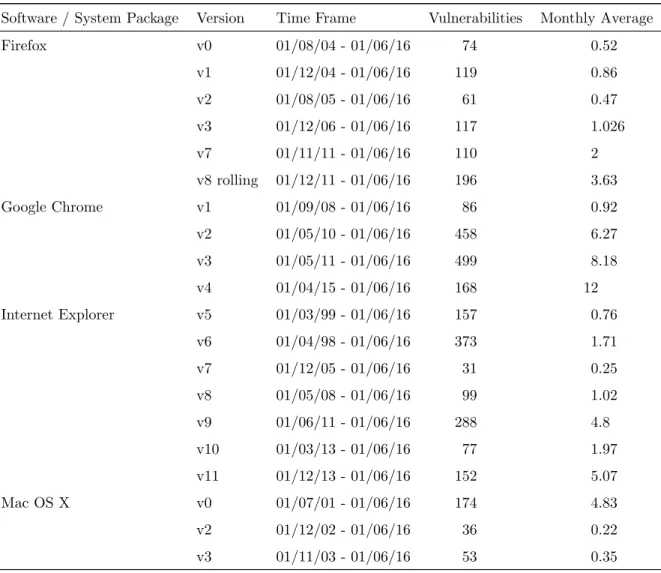
Table 4 shows the descriptive statistics of the used software and system packages.
Table 4: Descriptive Statistics
Software / System Package Version Time Frame Vulnerabilities Monthly Average
Firefox v0 01/08/04 - 01/06/16 74 0.52
v1 01/12/04 - 01/06/16 119 0.86
v2 01/08/05 - 01/06/16 61 0.47
v3 01/12/06 - 01/06/16 117 1.026
v7 01/11/11 - 01/06/16 110 2
v8 rolling 01/12/11 - 01/06/16 196 3.63
Google Chrome v1 01/09/08 - 01/06/16 86 0.92
v2 01/05/10 - 01/06/16 458 6.27
v3 01/05/11 - 01/06/16 499 8.18
v4 01/04/15 - 01/06/16 168 12
Internet Explorer v5 01/03/99 - 01/06/16 157 0.76
v6 01/04/98 - 01/06/16 373 1.71
v7 01/12/05 - 01/06/16 31 0.25
v8 01/05/08 - 01/06/16 99 1.02
v9 01/06/11 - 01/06/16 288 4.8
v10 01/03/13 - 01/06/16 77 1.97
v11 01/12/13 - 01/06/16 152 5.07
Mac OS X v0 01/07/01 - 01/06/16 174 4.83
v2 01/12/02 - 01/06/16 36 0.22
v3 01/11/03 - 01/06/16 53 0.35
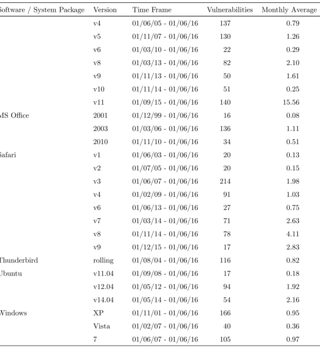
Table 4: Descriptive Statistics
Software / System Package Version Time Frame Vulnerabilities Monthly Average
v4 01/06/05 - 01/06/16 137 0.79
v5 01/11/07 - 01/06/16 130 1.26
v6 01/03/10 - 01/06/16 22 0.29
v8 01/03/13 - 01/06/16 82 2.10
v9 01/11/13 - 01/06/16 50 1.61
v10 01/11/14 - 01/06/16 51 0.25
v11 01/09/15 - 01/06/16 140 15.56
MS Office 2001 01/12/99 - 01/06/16 16 0.08
2003 01/03/06 - 01/06/16 136 1.11
2010 01/11/10 - 01/06/16 34 0.51
Safari v1 01/06/03 - 01/06/16 20 0.13
v2 01/07/05 - 01/06/16 20 0.15
v3 01/06/07 - 01/06/16 214 1.98
v4 01/02/09 - 01/06/16 91 1.03
v6 01/06/13 - 01/06/16 27 0.75
v7 01/03/14 - 01/06/16 71 2.63
v8 01/11/14 - 01/06/16 78 4.11
v9 01/12/15 - 01/06/16 17 2.83
Thunderbird rolling 01/08/04 - 01/06/16 116 0.82
Ubuntu v11.04 01/09/08 - 01/06/16 17 0.18
v12.04 01/05/12 - 01/06/16 94 1.92
v14.04 01/05/14 - 01/06/16 54 2.16
Windows XP 01/11/01 - 01/06/16 166 0.95
Vista 01/02/07 - 01/06/16 40 0.36
7 01/06/07 - 01/06/16 105 0.97
4. Empirical Results and Discussion
445
We predicted the number of IT security vulnerabilities based on the forecasting methodologies implemented in the R package “forecast” (Hyndman, 2017).
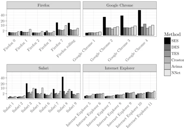
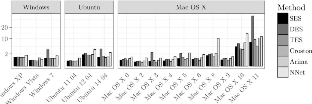
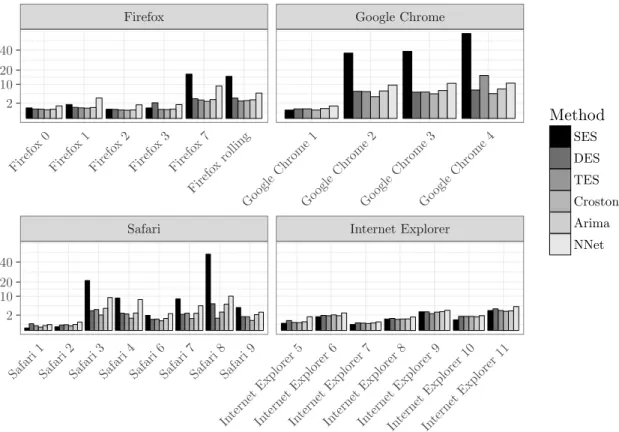
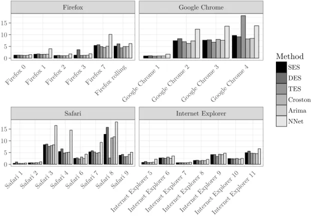
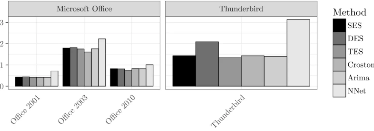
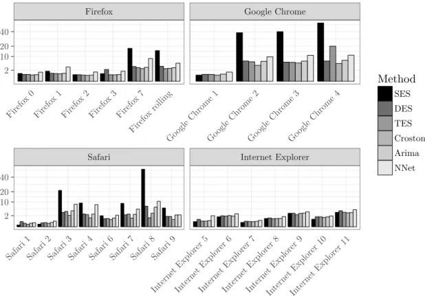
4.1. Results
Since forecasting research has shown that long-term forecasts are generally limited in their pre- dictive accuracy, we evaluated our methodologies on relatively short time frames forecasting one,
450
two, and three months ahead into the future (Leitch and Ernesttanner, 1995; ¨ Oller and Barot, 2000).
We could not find any substantial differences in forecasting accuracy between the shorter forecasting horizons of one or two months in comparison to the longer one of three months. Apart from the findings of prior research and the results of our own analysis, we consider a three-month forecasting horizon to strike a reasonable balance between having enough time to react and having accurate
455
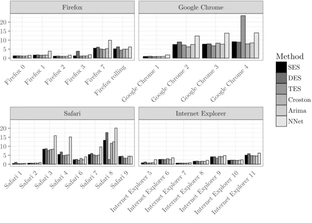
prediction accuracies for decision makers. Throughout the paper, forecasting accuracy (MAE and RMSE) is therefore reported for the entire time frame available (cf. Table 4). Figures 2 to 18 present the overall prediction accuracy (MAE and RMSE) for the analyzed software and system packages.
The figures are grouped according to application domains to facilitate comparisons between related software products. We show data that is subdivided into the major versions (x-axis) for the fore-
460
casting horizon of three months. 7 The absolute metrics’ scores are aggregated for the whole time frame as described in Table 4. The performance for the forecasting methodologies and the different versions of the system and software packages is provided in Table 5, 6, and 7.
Safari Internet Explorer
Firefox Google Chrome
Safari 1
Safari 2
Safari 3
Safari 4
Safari 6
Safari 7
Safari 8
Safari 9
In ternet E xplorer
5
In ternet E xplorer
6
In ternet E xplorer
7
In ternet E xplorer
8
In ternet Explorer
9
In ternet E xplorer
10
In ternet E xplorer
11 Firefo
x 0 Firefo
x 1 Firefo
x 2 Firefo
x 3 Firefo
x 7
Firefo x rolling
Go ogle Chrome
1
Go ogle Chrome
2
Go ogle Chrome
3
Go ogle Chrome
4 2
10 20 40
2 10 20 40
Method
SES DES TES Croston Arima NNet
Figure 2: Prediction Accuracy (MAE) for Browsers, h=1 (month)
7