Potassium-induced radioactivity in milk, rice and legumes

Potassium-induced radioactivity in milk, rice and legumes

Kaliuminduzierte Radioaktivit¨at in Milch, Reis und H ¨ ulsenfr ¨ uchten

Technische Universit¨at M¨unchen

Bachelor Thesis

by

Manuela Duda

18. August 2014

Max-Planck-Institut f¨ur Physik

Werner-Heisenberg-Institut

Contents

1 Introduction 5

1.1 Potassium

K . . . . 5 1.2 Samples . . . . 5 1.3 Structure of this thesis . . . . 5

2 Experimental Setup 6

2.1 Devices . . . . 6 2.2 Background reduction through shielding . . . . 7 2.3 Possible measurement configurations . . . . 8

3 Data taking 10

4 Analysis 12

4.1 Energy calibration . . . . 12 4.2 Number of counts in the signal peak . . . . 13 4.3 Potassium content . . . . 15

5 Results 17

5.1 K content in milk . . . . 17 5.2 K content in rice . . . . 18 5.3 K content in legumes . . . . 20

6 Other peaks 21

7 Summary 22

8 Appendix 23

1 Introduction

This thesis is about measurements of the potassium content in milk, rice and legumes. Potassium is an important mineral for the human body. It is essential for several physiological processes like nerve conduction, regulation of the water balance and blood pressure. The recommended daily allowance for potassium is 2.000 mg for an adult [1]. The potassium content of normal portions of the investigated consumables are compared to this value. To determine the potassium content, the natural radioactivity of potassium is exploited by analyzing spectra taken with a high purity germanium detector.

1.1 Potassium

K

40

19

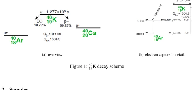
K is one of the isotopes of potassium. It is radioactive with a half-life of 1.27 billion years and has a natural abundance of 0.012 %. It has 19 protons and 21 neutrons. Figure 1 shows the decay scheme.

K decays to 89.28 % via β

decay to the ground state of

Ca. In 10.72 %, it decays via electron capture to an excited state of

Ar, which emits a gamma of 1460 keV [2].

(a) overview (b) electron capture in detail

Figure 1:

K decay scheme

1.2 Samples

The following samples were measured. They were selected to represent common dietary choices of potassium rich consumables.

UHT-milk Rice Dried Legumes

Full cream milk (3.5 % fat) Basmati rice from Pakistan (Asia) White beans Low-fat milk (1.5 % fat) Basmati rice from India (Asia) Green peas Lactose-free milk (1.5 % fat) Long grain rice from Italy (Europe) Red lentils

Sushi rice from California (USA)

Table 9 in the appendix shows the original names and brands of the food samples.

1.3 Structure of this thesis

In the following sections, the experimental setup, data taking, data analysis and results are presented.

2 Experimental Setup

2.1 Devices

To measure the gamma emitted by the potassium, the following components are needed:

• Germanium detector: The germanium detector used was produced by Canberra. It is a so called REGe (Reverse-Electrode Coaxial Germanium Detector). In this n-type REGe, the p + electrode (ion-implanted boron) is on the outside and the n + contact (di ff used lithium) is on the inside.

Figure 2 shows a schematic of the detector. This design features a thin window allowing for a low measuring threshold [3].

Figure 2: Shematic view of the REGe detector used, based on [4]

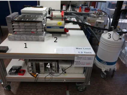
• Vacuum cryostat and cooling finger: Due to the relatively small band gap of Germanium, the de- tector has to be cooled to about 100 K to reduce the thermal generation of charge carriers [3]. The detector is cooled with a cooling finger. The cooling finger is submerged in liquid nitrogen at 77 K in the vacuum cryostat (number (2) in Fig. 3).

To refill the cryostat, a movable dewar (number (3) in Fig. 3) is used. It holds 60 l and is refilled once a week to provide enough LN

for this and other cryostats.

• Shielding: To reduce environmental background, there is a 8.5 cm thick lead castle. It is marked with (1) in Fig. 3. Lead (

Pb) is very dense (11,342

at 20

C [5]), thus, it is a good choice of shielding material. Inside the castle is a box made of copper. This prevents contact between the food samples and the toxic lead. The e ff ectiveness of the shield will be discussed in section 2.2.

• HV supply: The HV supply provides a voltage of -4500 V. This voltage is needed to ensure that the detector is fully depleted and works stably. The voltage also provides the electric field in the detector, which supports the collection of charge carriers [6].

• Data aquisition system (DAQ): The DAQ system is called Pixie-4. It is a multi-channel DAQ

produced by XIA [7]. To read out the REGe, only one channel is necessary. For each event, time

and energy are stored to facilitate a spectral analysis.

Figure 3: Measurement setup: (1) lead castle, (2) cryostat, (3) dewar and (4) HV supply and DAQ

2.2 Background reduction through shielding

As potassium is present in many objects, it contributes significantly to the environmental background. To reduce this background, there is a lead castle for shielding. To study the e ff ectiveness of the shield, three measurements were made with different setups. First measurement was without any shield. Another measurement was taken without the lid and one with the lead castle completely closed (Fig. 4). In Fig. 5, the respective spectra are shown. The peak at 1460 keV as well as the Compton background in that energy region are reduced by more than a factor of 10 by the shield. The good shield makes it possible to measure the activity of food with a low potassium content like milk.

For all further measurements, individual background measurements were made. They were scaled with the lifetime and subtracted from the time scaled sample measurements.

(a) Without any shield (b) Lid open (c) Lid closed

Figure 4: Setup for different levels of shielding

Figure 5: Environmental background measured with no shield (green), lead castle with open lid (blue) and lead castle with closed lid (orange)

2.3 Possible measurement configurations

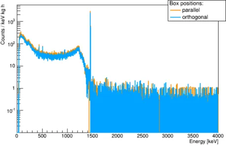
For the measurements, a Lock&Lock

box (HPL812) with a volume of V = 1 l was used. The box was placed in front of the detector in two di ff erent configurations (Fig. 6).

(a) Box parallel to the window (b) Box orthogonal to the window

Figure 6: Di ff erent box configurations

The goal was to maximize the count rate, which is influenced by the geometrical acceptance. For a point source at a distance from the detector, d

, the geometrical acceptance would be

= S

S

= π · r

4π · d

, (1)

where r

= 35 mm is the radius of the detector. The distance of the center of the box in the parallel position is d

= 98 mm and in the orthogonal position d

= 113 mm. Using equation 1, this results in

= 3.2 % and

= 2.4 %. This crude estimate considers only gammas entering the detector through the window. It also does not consider the real geometry of the container and the self absorption. The self absorption, however, is less than 5 % and will be neglected throughout.

To determine the real acceptance, the box was completely filled with potassium chloride (KCl). Equa- tion 2 provides the mass of potassium in KCl from the molar masses, m

= 39.10 u and m

= 35.45 u, where u is the unified atomic mass unit (1 u = 1.661 · 10

kg), and the level of impurity, i

= 0.00258, specified in the data sheet [8]:

m

= m

· (1 − i

) · m

m

+ m

, (2)

where m

= 627, 8 g is the mass of potassium in m

= 1200.1 g of KCl salt. To obtain the number of photons in one second, the activity, A, must be calculated:

A = m

m

· N

· ln(2) t

2

, (3)

where m

is the mass of

K. The Avogadro constant is N

= 6.022 · 10

. Potassium-40 decays with a branching ratio of BR

= 10.67 % to Argon, has a half-time of t

2

= 1.248 · 10

years and a molar mass of m

= 39.96 u. Its natural abundance is a

= 0.012 %. The activity of the box full of KCl becomes:

A = m

· a

m

· N

· ln(2) t

2

· BR

= 2132 Bq . (4)

In both configurations, parallel and orthogonal to the aluminium window, measurements were performed.

Also a background measurement with the empty box was made. The spectrum from 0 keV to the full ab- sorption peak of potassium at 1460 keV was analyzed. The sample measurements and the corresponding background measurement were normalized to their respective lifetimes. A list of measurements is given in Section 3.

The real acceptance,

, was determined from the background subtracted spectrum, integrated from 0 to 1465 keV to include the compton spectrum, the single and double escape peak and the full absorption peak:

= C

A , (5)

where C is the measured count rate per second.

The measurement yielded:

• In the parallel position, 26.16 photons per second were measured. That corresponds to

= (1.230 ± 0, 004) % (stat.).

• In the orthogonal position, 21.62 photons per second were measured. That corresponds to

= (1.010 ± 0, 004) % (stat.).

Considering the ration

real,orthogonal

, the systematic uncertainty on A, coming from measuring uncertainty on m

, drops out. The statistical uncertainty on each of about 0.004 % is small and thus, the di ff erence between

and

is significant.

The full spectra for the two configurations are shown in Figure 7. The parallel position was chosen for all further measurements. The values of

are significantly lower than the crude estimate. This is due to the large size of the box and a significant probability that a gamma entering the detector does not interact inside.

Figure 7: Normalized and background subtracted spectra for a container with 1 kg of KCl placed in front of the detector in two di ff erent orientations

3 Data taking

This section provides a detailed list of the measurements and the parameters relevant for data taking. The DAQ was operated with the following settings:

• Run type: Energy and time only

• Gain = 3

• Threshold = 20 ( ˆ = 280 ADC channels ˆ = 34 keV) [9]

Tables 1 – 4 provide an overview over the measurements. For every measurement, the date and the

lifetime are given. For sample measurements, the mass and the used background is also listed. The

backgrounds were measured close to the sample measurements with the cleaned and empty box. Their

lifetime is always significantly larger than those of the corresponding sample measurements. After the

milk measurements, the box was cleaned with water and cleanroom wipes ”Micropure”, class 100, made

of cellulose and polyester. After all other measurements, the box was cleaned with the cleanroom wipes

only. The first measurement was the calibration measurement with KCl (Table 1). The measurements of

the food samples are listed in Tables 2 (milk), 3 (rice) and 4 (legumes). The food was taken out of the

packaging and filled into the box without any treatment. The box was fully filled and measured in the

parallel position.

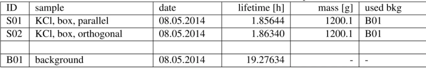
Table 1: Calibration with KCl in di ff erent container positions

ID sample date lifetime [h] mass [g] used bkg

S01 KCl, box, parallel 08.05.2014 1.85644 1200.1 B01

S02 KCl, box, orthogonal 08.05.2014 1.86340 1200.1 B01

B01 background 08.05.2014 19.27634 - -

Table 2: UHT-milk

ID sample date lifetime [h] mass [g] used bkg

S03 full cream milk 15.05.2014 23.98344 1027.8 B02

S04 low-fat milk 18.05.2014 17.88926 1029.2 B02

S05 lactose-free milk 28.05.2014 19.61853 1029.1 B03

B02 background 16.05.2014 54.30156 - -

B03 background 29.05.2014 94.01584 - -

Table 3: Rice from di ff erent countries

ID sample date lifetime [h] mass [g] used bkg

S06 basmati rice from Pakistan 11.06.2014 23.97631 900.0 B04

S07 basmati rice from India 16.06.2014 43.41028 900.0 B04

S08 long grain rice from Italy 18.06.2014 24.31156 900.0 B05 S09 sushi rice from California 08.07.2014 140.20860 974,3 B06

B04 background 12.06.2014 95.60041 - -

B05 background 19.06.2014 100.19971 - -

B06 background 25.06.2014 312.85202 - -

Table 4: Di ff erent legumes

ID sample date lifetime [h] mass [g] used bkg

S10 white beans 26.05.2014 2.57342 900.0 B07

S11 green peas 26.05.2014 3.30631 900.0 B07

S12 red lentils 27.05.2014 12.56044 900.0 B07

B07 background 26.05.2014 28.07208 - -

4 Analysis

4.1 Energy calibration

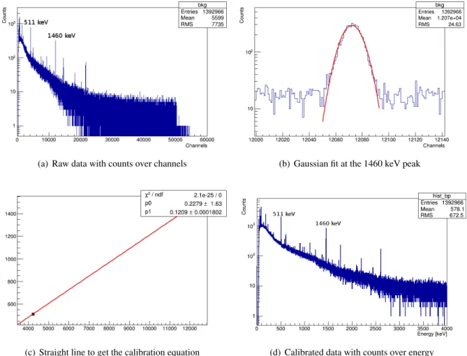
The DAQ provides the number of events per ADC-channel. For further analysis, the data have to be calibrated, i.e. the channel numbers have to be converted into energies. The tool used to handle spectra is ROOT [10]. Figure 8a shows the raw spectrum for measurement S09. The two peaks used for calibration are at channel numbers 4223 and 12070. They are fitted with a Gauss-function. Figure 8b shows the result for the peak at 12070. The two peaks are identified as the 511 keV and 1460 keV peaks:

• The 511 keV peak is caused by annihilation of positrons produced by pair production outside the detector [6].

• The 1460 keV peak is the full absorption peak of

K.

(a) Raw data with counts over channels (b) Gaussian fit at the 1460 keV peak

(c) Straight line to get the calibration equation (d) Calibrated data with counts over energy

Figure 8: Calibration process exemplary for sushi rice

The mean value of the Gaussians are matched with the energies: (511 keV, 4223) and (1460 keV, 12070).

The two points are drawn in an energy-channel-diagram (Fig. 8c). A linear fit gives the y-intercept,

p

, and the slope p

. The fit parameter p

is consistent with 0 within its errors and this validates the

linearity. Table 10 in the appendix provides the calibration parameters for all data sets. The calibration

was extremely stable throughout the data taking. The calibrated spectrum (Fig. 8d) has a modified y-scale

as energy and channel bins have di ff erent widths.

4.2 Number of counts in the signal peak

The 1460 keV peaks are evaluated. The number of events in the peak is determined for the sample and the background measurements. The fit function is a sum of terms corresponding to different physical contributions [11]:

• Gaussian shape: For an ideal detector, a Gaussian with a small natural width due to the statistics of charge carrier creation is expected for full absorption. It is broadened by noise due to incomplete charge carrier collection and electronics.

• Exponentially decaying distribution: Regional incomplete charge collection and pile-up effects can remove counts from the peak. This produces an exponential decaying distribution below the peak.

The Gaussian shape plus this distribution results in a peak with a roughly Gaussian shape but skewed or broadened on the low energy side.

• Step function: The Compton background in the detector can create an apparent step function un- derneath the peak.

• Polynomial: The background term for the continuum is represented by a first order polynomial.

This function is the only one, that does not get folded into the Gauss function.

The sum of these four terms, illustrated in Fig. 9, is:

F( x, σ, b) = A · (1 − F

) 1 σ √

2π exp

− x − µ

√ 2σ

+ A · F

exp(

+

)(1 − erf(

+

) 2b

+ I · 0.5 erfc( x − µ

√ 2σ ) ,

(6)

where A is the area under the peak, F

is the skew factor, σ is the standard deviation, x is the energy, µ is the center of the fit, I is the height of the step and b is the skew width multiplied by σ.

The program package ROOT [10] is used for the fit with the internal fit setting ”Maximum Likelihood”.

ROOT integrates the fit functions and calculates the counts under the peaks with their uncertainties in the unscaled spectra. The uncertainties are approximately

N

. Two fitted spectra are shown in Fig. 10.

The counts and their uncertainties are scaled with the respective lifetimes. The count rate for the back- ground, c

, is subtracted from the count rate for the signal+background spectrum, c

, to obtain the count rate for the signal, c

:

c

= c

− c

. (7)

The uncertainty is calculated with error propagation:

∆ c

= q

∆ c

+ ∆ c

. (8)

Figure 9: Illustration of terms used in the fitting function, based on [11]

(a) raw Signal+bkg for sushi rice (b) Bkg for sushi rice, unscaled

Figure 10: Area under the peak fit exemplary for sushi rice. Fit parameters:

peak1 center ˆ = µ, peak1 area ˆ = A, peak1 sigma ˆ = σ, peak1 stepAmpl ˆ = I.

In order to compare the food samples, the count rates have to be scaled with the respective masses:

c

= c

m . (9)

The masses are measured with an uncertainty of ∆ m = 0.1 g. The uncertainty is calculated as:

∆ c

= s

∆ c

c

+ ∆ m m

· c

. (10)

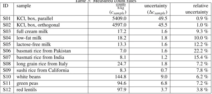
The results are presented in Table 5. Table 11 in the appendix provides information about the count rates before subtraction.

Table 5: Measured count rates

ID sample

(c

)

uncertainty (∆ c

)

relative uncertainty

S01 KCl, box, parallel 5409.0 49.5 0.9 %

S02 KCl, box, orthogonal 4597.0 45.5 1.0 %

S03 full cream milk 17.2 1.6 9.3 %

S04 low-fat milk 18.2 1.8 10.0 %

S05 lactose-free milk 13.3 1.6 12.2 %

S06 basmati rice from Pakistan 7.0 1.6 22.2 %

S07 basmati rice from India 8.1 1.2 15.4 %

S08 long grain rice from Italy 24.7 1.8 7.2 %

S09 sushi rice from California 8.3 0.7 7.8 %

S10 white beans 144.8 9.0 6.2 %

S11 green peas 94.6 6.8 7.2 %

S12 red lentils 97.9 3.7 3.8 %

4.3 Potassium content

In order to determine the potassium content in the food samples, the measured food data are calibrated with the KCl data:

c

m(K)

= c

m(K)

⇒ m(K)

= c

· m(K)

c

=: c

·

, (11) where:

• m(K)

is the mass of potassium in the food sample;

• m(K)

= m

· (1 − i

) ·

mol,K+mmol,Cl

= (627.8 ± 0.6) g is the mass of potassium in the salt;

• c

= (5409 ± 50)

under the KCl peak;

• c

are the measurements listed in Table 5.

Therefore, the uncertainty on m(K)

is calculated as:

∆ m(K)

= s

∆ i

1 − i

+ ∆ m

m

· m(K)

= 0, 6 g , (12) where i

= 0.003, ∆ i

= 0.001, m

= 1200.1 g and ∆ m

= 0.1 g, and the uncertainty on

mmol,K

m_mol,K+m_mol,Cl

is assumed to be zero.

With the values from Table 5 for S01

= 0.0967

. (13)

The asymmetry of the uncertainty is small due to the high statistics of the measurement. This uncertainty is used as a correlated systematic uncertainty of all measurements from here on.

The uncertainties on the m(K)

values are dominated by the statistical uncertainties on the count rates, as the measurement uncertainty on m is comparatively small. Therefore all results will be quoted as

m(K)

= m ± σ

−σsys,−

. (14)

5 Results

In the following sections, the measured potassium content and its uncertainty of the di ff erent food sam- ples are listed. The uncertainties are symmetric, because they are dominated by the statistic uncertainties.

All the results are given in mg per 100 g of the food samples. Also given are expected values [12].

5.1 K content in milk

Table 6 and Fig. 11 show the measured potassium content in milk with its uncertainty together with the expectations [12]. There is no significant di ff erence between the three kinds of milk. The measure- ments agree with each other and with the expectation. If milk is considered as part of the potassium balance, a glass of milk provides about 300 mg of potassium, i.e. 15 % of the recommended daily intake, independent of the fat content.

Figure 11: Potassium content in milk in %. The inner errorbars represent the statistical uncertainties, the

outer bars represent the statistical and systematic uncertainties added in quadrature. The difference is not

visible for all points.

Table 6: K content in milk

ID sample Exp. K Meas. K σ

σ

σ

content content [

] [

] [

] [

] [

]

S03 full cream milk 150 166 15 1 16

S04 low-fat milk 150 176 17 2 17

S05 lactose-free milk 150 129 15 1 16

5.2 K content in rice

The expectation is different for husked and unhusked rice. For basmati and sushi rice, the value for husked rice is taken. For the long grain rice, the expectation for unhusked rice is relevant. Table 3 and Fig. 12 show the results.

Table 7: K content in rice

ID sample Exp. K Meas. K σ

σ

σ

content content [

] [

] [

] [

] [

]

S06 basmati rice from Pakistan 103 68 15 1 15

S07 basmati rice from India 103 78 12 1 12

S08 long grain rice from Italy 150 239 17 2 18

S09 sushi rice from California 103 80 7 1 7

All husked kinds of rice show potassium contents slightly below expectation. Basmati rice is a kind of long grain rice, but the difference between basmati and long grain rice is pronounced. This demonstrates that the kind of rice is not the deciding factor, but the husking is. That confirms that most of the dietary minerals are in the shell.

The origin of the rice could also have an e ff ect. The rice plant takes the potassium from the soil and stores it in the grains. In Fig. 13, the values of the three husked rices are drawn with their weighted average and the uncertainties. No significant variations are observed. Any influence of the soil is too small to be detectable at this level.

A portion of 100 g of husked rice only provides about 4 % of the recommended daily intake of 2 g of

potassium.

Figure 12: Potassium content in rice in %. Other details as in Fig. 11.

Figure 13: The values of the three husked rices with uncertainties and their weighted average (red line)

with its uncertainty (yellow box). Other details as in Fig. 11.

5.3 K content in legumes

All legumes have a relatively high potassium content compared to the other samples. They are listed in Table 8 and are shown in Fig. 14. Green peas and red lentils have the same value within uncertainties.

White beans provide significantly more potassium.

To meet the daily requirement of 2 g of potassium, 219 g of peas, 211 g of lentils or 143 g of beans have to be eaten. This is certainly an easy way to consume the necessary potassium.

Table 8: K content in legumes

ID sample Exp. K Meas. K σ

σ

σ

content content [

] [

] [

] [

] [

]

S10 white beans 1336 1401 87 12 88

S11 green peas 940 915 66 8 66

S12 red lentils 840 946 36 8 37

Figure 14: Potassium content in beans, peas and lentils in %. Other details as in Fig. 11.

6 Other peaks

In principle, the spectra could show lines of minerals other than potassium related to soil conditions or other environmental influences.

Fig. 15 shows the spectrum of the sushi rice, where the background is not yet subtracted. There are many peaks apart from the

K peak. The most pronounced ones are caused by the isotopes

Bi and

Tl.

After the background subtraction, the spectrum depicted in Fig. 16 shows no prominent lines. There is only a small indication of a

Bi line at 609 keV. However as the other

Bi lines are missing, this is most likely a background variation.

Figure 15: Peaks in spectrum of S09, not background subtracted

All background subtracted spectra are shown in the appendix. Milk and legume spectra (Fig. 17, and 19) do not show any features apart from the

K peak. Also basmati rice from Pakistan (Fig. 18a) has no peaks apart from the

K peak. Basmati rice from India has a small

Bi peak at 2204 keV. However, it is most likely due to a background fluctuation as no other

Bi lines are present in the subtracted spectrum.

The long grain rice from Italy (Fig. 18c) shows an indication of an enhanced

Tl line at 2614.5 keV, a

product of the

Th decay chain [13].

Figure 16: Background subtracted spectrum of S09. The 609 keV line from

Bi is marked.

7 Summary

Measurements of gamma spectra of milk, rice and legumes with a high purity germanium detector were presented. The gamma line at 1460 keV from

K was used to determine the potassium content in the consumables.

The experimental setup comprises the germanium detector, a lead shield with space for sizeable samples and the required electronics and data aquisition. The placement of the samples was optimized and the effectiveness of the shield was demonstrated. The system was calibrated by measuring the spectrum of a large sample of KCl. The various measurements of consumables provide information about their potassium content at the 10 % level. The measurement uncertainties are dominated by statistics.

The results demonstrate the different potassium content in the food samples. Among all samples, legumes have the highest potassium content. All measured values are near the expectations.

A search for other peaks in the spectra was performed. In all but one spectrum no indication for other

radioactive minerals was detected. Only Italian rice shows an indication for enhanced Thorium through

a peak associated with

Tl.

8 Appendix

Table 9: Original names and brands of the food samples

ID sample original name brand

S03 full cream milk Haltbare Vollmilch Milbona

S04 low-fat milk Haltbare fettarme Milch Milbona

S05 lactose-free milk Haltbare fettarme Milch, laktosefrei Milbona

S06 basmati rice from Pakistan Bio Basmatireis verivalBIO

S07 basmati rice from India Basmati Reis, Original, weiß BioGourmet S08 long grain rice from Italy Langkornreis, natur BioGourmet S09 sushi rice from California Sushi Reis, Koshihikari Reishunger

S10 white beans Weiße Bohnen M¨ullers M¨uhle

S11 green peas Gr¨une Erbsen M¨ullers M¨uhle

S12 red lentils Rote Linsen M¨ullers M¨uhle

Table 10: Energy calibration details

ID sample ADC channel

for 511 keV

ADC channel for 1460 keV

y-intercept p

slope p

S01 KCl, box, parallel 4222.61 12064.6 0.000000 0.121015

S02 KCl, box, orthogonal 4222.75 12065.0 -1.082630 0.121268

S03 full cream milk 4224.01 12071.9 0.214873 0.120924

S04 low-fat milk 4224.17 12072.3 0.211146 0.120921

S05 lactose-free milk 4222.11 12068.5 0.347026 0.120947

S06 basmati rice from Pakistan 4223.23 12069.4 0.192590 0.120950

S07 basmati rice from India 4223.18 12069.6 0.219565 0.120947

S08 long grain rice from Italy 4222.80 12069.5 0.283750 0.120943 S09 sushi rice from California 4224.08 12072.3 0.227886 0.120919

S10 white beans 4225.98 12073.3 -0.060466 0.120933

S11 green peas 4225.14 12071.7 -0.008373 0.120945

S12 red lentils 4222.93 12070.0 0.292109 0.120937

B01 background 4221.83 12065.4 0.197308 0.120991

B02 background 4223.97 12071.9 0.222313 0.120924

B03 background 4221.77 12068.5 0.410273 0.120942

B04 background 4223.05 12069.4 0.230731 0.120948

B05 background 4223.29 12069.5 0.192590 0.120950

B06 background 4223.50 12071.0 0.251163 0.120930

B07 background 4224.59 12071.2 0.061402 0.120944

Table 11: Lifetime scaled counts in signal+bkg & bkg–peak and the calculated counts from signal ID sample c

∆ c

c

∆ c

c

∆ c

S01 KCl, box, parallel 6517.31 59.35 25.99 1.28 6491.32 59.37

S02 KCl, box, orthogonal 5542.90 54.64 25.99 1.28 5516.91 54.65

S03 full cream milk 45.18 1.44 27.54 0.77 17.64 1.63

S04 low-fat milk 46.29 1.70 27.54 0.77 18.75 1.87

S05 lactose-free milk 42.31 1.56 28.62 0.60 13.69 1.67

S06 basmati rice from Pakistan 33.65 1.27 27.36 0.58 6.29 1.40

S07 basmati rice from India 34.63 0.96 27.36 0.58 7.27 1.12

S08 long grain rice from Italien 49.68 1.50 27.41 0.57 22.27 1.61

S09 sushi rice from California 36.08 0.54 27.97 0.33 8.11 0.64

S10 white beans 158.62 8.03 28.26 1.10 130.36 8.10

S11 green peas 113.43 6.00 28.26 1.10 85.17 6.10

S12 red lentils 116.34 3.11 28.26 1.10 88.08 3.30

(a) Full cream milk (b) Low-fat milk

(c) Lactose-free milk

Figure 17: Background subtracted milk spectra

(a) Basmati, Pakistan (b) Basmati, India

(c) Long grain, Italy (d) Sushi, California

Figure 18: Background subtracted rice spectra with some other marked peaks than potassium

(a) White beans (b) Green peas

(c) Red lentils

Figure 19: Background subtracted legume spectra

References

[1] Deutsche Gesellschaft fuer Ernaehrung e. V., Referenzwerte fuer die Naehrsto ff zufuhr, accessed on 28/07/2014, URL http://www.dge.de/modules.php?name=Content&pa=showpage&pid=

3&page=5.

[2] R. B. Firestone, Table of Isotopes, vol. 1 (1996), 8th ed.

[3] I. Canberra Industries, Germanium Detectors, User’s Manual (2003).

[4] I. Canberra Industries, Reverse Electrode Coaxial Ge Detectors (REGe), accessed on 28/07/2014, URL http://www.canberra.com/products/detectors/pdf/

REGe-Detector-SS-C40432.pdf.

[5] Je ff erson Lab, The element Lead, accessed on 01 / 08 / 2014, URL http://education.jlab.org/

itselemental/ele082.html.

[6] G. F. Knoll, Radiation Detection and Measurement (2000), 3rd ed.

[7] A. Glueck, Automatisierung der Messprozesse des GALATEA Teststandes (2009).

[8] AppliChem, Kaliumchlorid reinst Ph. Eur., USP (2014).

[9] C. Carissimo, Final Report of Summer Internship (2013), unpublished.

[10] CERN, User’s Guide ROOT - Data Analysis Framework (2014).

[11] G. W. Philipps and K. W. Marlow (1976).

[12] Berliner Medizinredaktion, Naehrsto ff datenbank - Kaliumgehalt in Lebensmitteln, accessed on 05 / 08 / 2014, URL http://www.dialyse.de/datenbank/.

[13] Idaho National Engineering & Environmental Laboratory, Gamma-ray Spectrum Catalogue (1998),

4th ed.