DISCUSSION PAPER SERIES
Forschungsinstitut zur Zukunft der Arbeit Institute for the Study of Labor
ORU Analyses of Immigrant Earnings in Australia, with International Comparisons
IZA DP No. 4422
September 2009 Barry R. Chiswick Paul W. Miller
ORU Analyses of Immigrant Earnings in Australia, with International Comparisons
Barry R. Chiswick
University of Illinois at Chicago and IZA
Paul W. Miller
University of Western Australia and IZA
Discussion Paper No. 4422 September 2009
IZA P.O. Box 7240
53072 Bonn Germany
Phone: +49-228-3894-0 Fax: +49-228-3894-180
E-mail: iza@iza.org
Any opinions expressed here are those of the author(s) and not those of IZA. Research published in this series may include views on policy, but the institute itself takes no institutional policy positions.
The Institute for the Study of Labor (IZA) in Bonn is a local and virtual international research center and a place of communication between science, politics and business. IZA is an independent nonprofit organization supported by Deutsche Post Foundation. The center is associated with the University of Bonn and offers a stimulating research environment through its international network, workshops and conferences, data service, project support, research visits and doctoral program. IZA engages in (i) original and internationally competitive research in all fields of labor economics, (ii) development of policy concepts, and (iii) dissemination of research results and concepts to the interested public.
IZA Discussion Papers often represent preliminary work and are circulated to encourage discussion.
Citation of such a paper should account for its provisional character. A revised version may be available directly from the author.
IZA Discussion Paper No. 4422 September 2009
ABSTRACT
ORU Analyses of Immigrant Earnings in Australia, with International Comparisons
*This paper examines the way immigrant earnings are determined in Australia. It uses the overeducation/required education/undereducation (ORU) framework (Hartog, 2000) and a decomposition of the native-born/foreign-born differential in the payoff to schooling developed by Chiswick and Miller (2008). This decomposition links overeducation to the less-than- perfect international transferability of immigrants’ human capital, and undereducation to favorable selection in immigration. Comparisons are offered with findings from analyses for the US and Canada to enable assessment of the relative impacts of favorable selection and the limited international transferability of human capital to the lower payoff to schooling for the foreign born. The sensitivity of the results of the decomposition to several measurement issues is assessed.
JEL Classification: F22, I21, J24, J31, J61
Keywords: immigrants, schooling, occupations, earnings, rates of return, selectivity, skill transferability, ORU analysis
Corresponding author:
Barry R. Chiswick
Department of Economics University of Illinois at Chicago 601 S. Morgan Street
Chicago, IL 60607-7121 USA
E-mail: brchis@uic.edu
September 2009 ORU ANALYSES OF IMMIGRANT EARNINGS IN AUSTRALIA,
WITH INTERNATIONAL COMPARISONS I. INTRODUCTION
A relatively low payoff to schooling for the foreign born is a feature of studies of the comparative labor market performance of the foreign born in all major immigrant receiving countries. In Chiswick’s (1978) pioneering study, based on the 1970 US Census, the partial effect of a year of schooling on earnings for the US native born was 7.2 percent, and that for the foreign born 5.7 percent. Baker and Benjamin (1994) report that the partial effect of years of schooling on earnings in the Canadian labor market was 7.3 percent for natives and 4.8 percent for immigrants in 1971, 6.6 percent and 4.4 percent, respectively, for these groups in 1981, and 7.6 percent and 4.9 percent respectively for the two groups in 1986. Similar findings have been reported for the United Kingdom by Chiswick (1980), for Australia by Beggs and Chapman (1988), for Israel by Chiswick (1979) and for Germany by Dustmann (1993).
Chiswick and Miller (2008) investigate this feature of the immigrant labor market experience in the US. They draw upon insights from the undereducation/overeducation literature (see Hartog, 2000) to propose a decomposition of the different payoffs to schooling for immigrant groups. This decomposition was applied to data from the 2000 US Census to show that the lower payoff to schooling for the foreign born in the US is linked to the labor market outcomes of immigrants who are not correctly matched to the usual educational standards of the jobs they hold, either because they have too much education (e.g., a person with a foreign law degree working as a law clerk) or too little education (e.g., a person with eight years of education working in a job where the usual schooling level is 12 years). The Chiswick-Miller decomposition appears to provide a quantification of the labor market
impacts of both the more intense favorable selection in migration among the foreign born, and of the non-recognition of foreign educational qualifications.
This paper applies the Chiswick and Miller (2008) decomposition to the Australian labor market. This enables an assessment of the roles of overeducation and undereducation in the determination of immigrants’ earnings in Australia, and, by implication, of the contributions of the less-than-perfect international transferability of immigrants’ human capital and selection in immigration to the lower payoff to immigrants’ schooling than for the native born. Comparisons are provided to the findings from similar studies for the US and Canada to permit assessment of the importance to the structure of immigrant earnings of the different systems for allocating visas in these countries—largely family reunion in the US, and points testing for a major component of the immigrant flows in Australia and Canada.
The robustness of the findings to alternative measures of undereducation and overeducation is also examined.
The paper is structured as follows. Section II provides an overview of the Chiswick and Miller (2008) decomposition and the methodological issues that are examined in the current study. Section III reviews the 2001 Australian Census of Population and Housing data to be used in the statistical analysis, while Section IV presents the statistical results for a conventional study of immigrant labor market outcomes, and for two alternative approaches with the undereducation/overeducation methodology. Section V provides the application of the Chiswick-Miller decomposition of the differences in payoffs to education for birthplace groups, again for the two alternative approaches utilized in the regression analyses presented in the previous section. Comparisons of the findings for Australia with similar sets of results for Canada and the US are provided in Section VI. Section VII presents a summary and conclusion.
II. THE CHISWICK-MILLER DECOMPOSITION: METHODOLOGICAL ISSUES A. The Decomposition
The starting point of the Chiswick and Miller (2008) decomposition is the Overeducation/Required education/Undereducation (ORU) specification of the human capital earnings equation (see Hartog, 2000). This modifies the conventional human capital earnings equation through the use of three schooling variables, S So, r and Su, in place of a single variable for the worker’s actual years of schooling (Si).1 Srrepresents the years of education that is usual in, or required by, the job as determined by one of the procedures to be discussed below,2 So denotes the number of years of overeducation (i.e., the individual’s actual education less that required or usual for their job where this amount is positive, and So is zero otherwise), and Su is the number of years of undereducation (i.e., the usual or required education in the job less the individual’s actual education where this magnitude is positive, and it is zero otherwise). That is:
lnWiXioSoirSriuSuii (1)
The estimated parameters, o, r and u, together with sample values of So, Sr and Su, provide the basis of the Chiswick and Miller (2008) decomposition. This can be explained with reference to Figure 1. This contains hypothetical earnings for five types of workers.
Workers A, B and C have levels of education (10, 12 and 14 years, respectively) that are
1The conventional equation takes the following form: lnWi XiSii , where Wi denotes the wage rate of individual i, Xi is a vector of variables (other than level of education) that affect earnings, and Si represents the individual’s years of education. and are parameters to be estimated and i is a random error term. records the payoff to schooling, which, under the assumptions set out in Becker and Chiswick (1966), can be interpreted as the rate of return to investments in formal schooling.
2 The literature uses “required” for this standard. However, as it is possible to work in the occupation with fewer years of schooling than the standard, alternative terms such as “usual”, “reference” or “standard” might be preferred.
assumed to be exactly equal to the levels that are usual in their employment. That is, they are correctly matched to the educational requirements of their jobs. Type D workers are, like the Type B workers, in jobs that require 12 years of education. However, unlike the Type B workers who have 12 years of education, Type D workers have only 10 years of education.
That is, they are undereducated by two years. Undereducation is generally a characteristic among individuals with low education levels. Type E workers are also, like Type B workers, in jobs that require 12 years of education. However, Type E workers are assumed to have 14 years of education. Hence, they are overeducated by two years. Overeducation is generally a characteristic among individuals with high education levels. The native born are denoted by NB in the figure and the foreign born by FB. The placement of workers in Figure 1 reflects the typical results from the ORU literature. Thus, the figure illustrates three key findings.3
First, there are sizeable earnings increments to correctly matched education (compare workers of Types A, B and C). In the Chiswick and Miller (2008) analysis for the US, these increments are essentially the same for the native born and foreign born, being around 15 percent higher earnings for each year of correctly matched education. Similar findings are reported below for the Australian labor market.
Second, undereducated workers, such as Type D workers, with 10 years of education, but working in an occupation where it is usual to have 12 years of education, earn more than workers who have 10 years of education and work in an occupation where it is usual to have 10 years of education (Type A), but they earn less than those with whom they share an occupation who have the correct (12 years) level of education for that occupation (Type C).
The undereducated from both birthplace groups are associated with relatively high earnings compared with those with the same level of education that are correctly matched. This earnings advantage is argued by Chiswick and Miller (2008) to be associated with
3 Parts of this discussion are drawn from Chiswick and Miller (2008).
unobservables that the undereducated are disproportionately endowed with that enable them to be employed in the higher-level occupation. Note, however, that the undereducated foreign born are generally reported to do better than the undereducated native born, and this is held to be associated with the foreign born being self-selected to migrate on the basis of unobserved characteristics that are positively correlated with earnings (e.g., motivation, perseverance, ability).
Figure 1
Earnings Situations of Hypothetical Workers
Third, overeducated workers, for example the Type E workers, with 14 years of education who work in an occupation where it is usual to have only 12 years of education, earn more than the workers with whom they share an occupation who have the correct level of education for that occupation (Type B), but they earn far less than workers with 14 years of education who are correctly matched in an occupation (Type C). The earnings disadvantage for these overeducated workers is greater for the foreign born than for the native born, and
Earnings ($)
Actual Years of Education
10 12 14
ANB, AFB
BNB, BFB
ENB EFB
CNB, CFB
DFB DNB
Native Born
Foreign Born
this is linked by Chiswick and Miller (2008) to the less-than-perfect international transferability of skills possessed by the foreign born.
The return to reference years of education is given by the slope of the line through points A, B and C. In comparison, the return to actual years of education will be derived from earnings-years of education relationships based on averages of the earnings for the workers described above at each level of education (e.g., average for Type A and Type D workers at 10 years of education, average for Type C and Type E workers at 14 years of education). This will therefore depend on both the estimated earnings effects associated with mismatched education, and the number of workers in each education category. As the estimated earnings of undereducated workers are above those for correctly matched workers, and the estimated earnings of overeducated workers are below those for correctly matched workers, the return to actual years of education will be lower than the return to reference years of education.
Hypothetical earnings-actual years of education relationships for the native born (the solid line) and foreign born (the dashed line) are included in Figure 1.
The mean earnings of workers at each education level needed to find the payoff to actual years of education can be computed from equation (1). This is illustrated with reference to the foreign born, though the application to the native born is straightforward.
The procedure is as follows
a. First, in order to remove the effects of characteristics other than educational attainment, each worker is assigned the sample means for each of their non-education variables.
b. Second, workers at each educational attainment are assumed to have the distribution across the overeducation, reference levels of education and undereducation categories specific to the foreign born at the particular education level.
c. Third, the effects on earnings of variables in equation (1), including overeducation, reference levels of education and undereducation, are given by the estimates for the relevant total foreign-born sample (e.g., either for English-speaking countries or for non- English-speaking countries).
d. On the basis of the assumptions listed in (a) to (c) above, use equation (1) to predict earnings at each level of education (e.g., 10, 12, 14 etc.).
The predicted mean logarithm of earnings from step (d) at each education level can then be related to the level of education in a linear regression. This regression is weighted by the number of workers in each educational attainment category. The slope coefficient in this simple regression is a convenient way of establishing the “other things the same” payoff to education.
Once the benchmark payoff to education has been found using the framework set out above, values from the analysis of earnings for the native born are substituted into the algorithm to permit a control for native-born/foreign-born differences. Hence, in the first instance, another weighted linear regression is computed, where in step (c) the earnings effects associated with overeducation, correctly matched education and undereducation for the foreign born (i.e., o, r and u) are replaced with those estimated for the native born. This effectively assigns a foreign-born undereducated worker such as DFB in Figure 1 an earnings level of DNB in the same figure, and it assigns a foreign-born overeducated worker such as EFB in Figure 1 an earnings level of ENB. This will allow the effect of actual years of education on earnings to be estimated under the condition that these earnings effects in the ORU model are identical for both the native born and the foreign born.
The computation of the payoff to education next replaces the information on the distribution across the overeducation, correctly matched education and undereducation
categories (i.e., mean values of So, Sr and Su) for the foreign born within each category of education with the respective information for the native born at each educational attainment category (see step (b)). This will enable an assessment of the role that dissimilar levels of overeducation and undereducation within each educational attainment category for the foreign born and native born have in producing the well documented gap in the returns to schooling for the foreign born.
Lastly, the distribution of the native born across educational attainment categories is employed in place of that of the foreign born in computing the “other things the same” payoff to education. This ensures that this payoff is based on the same distribution across levels of educational attainments among both the native born and the foreign born, as well as resulting in the same overall levels of overeducation and undereducation for both groups. By construction, the payoff derived in this final step will be that for the native born.
B. Measurement of Reference Years of Education
An important consideration in the framework described above is obviously the measurement of the reference or usual level of education for a person’s job, and thus the extent of overeducation and undereducation. Three measures have been proposed. These are the worker self-assessment, job analysis, and realized matches procedures. The nature of the data employed in any given study generally dictates which of these procedures will be used.
Worker self-assessment is a subjective measurement, where individual workers are
asked to specify either the “required” level of education, or the rate of skill utilization, of their job. This method generally requires that the workers’ subjective assessment of his job is collected along with other data that could be used in the analysis. This prevents its application in the current analysis of census data.
Job Analysis is an assessment of the educational requirements for the job titles in an
occupational classification made by professional job analysts. The Australian Standard Classification of Occupations (ASCO), jointly produced by the Australian Bureau of Statistics and the (then) Department of Employment, Education, Training and Youth Affairs, is an example of this type of measure. This is a skill-based classification of the current minimum standards for all occupations in Australia. An advantage to this type of measure is that it can be readily formed with any data set that contains information on the occupation of employment that can be matched to the ASCO codes.
The realized matches procedure is an objective measurement of job requirements derived from the actual educational attainments of workers in each occupational category (Kiker et al., 1997). This procedure measures the job requirements by computing the mean (or modal) educational level for each occupation. The actual level of education for each worker is then compared to the mean (or modal) value to determine whether the worker is matched to the apparent standards of the job. Like the job analysis method, the realized matches procedure can be applied to any data set that contains information on the occupation of employment.
In this study both the realized matches and job analysis procedures are used to compute the reference or required levels of education for the jobs distinguished in the data set.4
III. DATA
The analyses presented below are based on the 2001 Australian Census of Population and Housing Household Sample File (HSF) (see Australian Bureau of Statistics, 2003). The
4 Chiswick and Miller (2009a) undertake analyses for the US based on the worker self-assessment and realized matches procedures. Both measures focus on the central tendency of the occupational requirements. They report that while the point estimates of the earnings effects differ between the methods, the general pattern in the findings was not sensitive to the choice of measure. This echoes Hartog’s (2000) earlier overview.
HSF contains a 1 percent sample of private dwellings, with their associated family and person records, and a 1 percent sample of persons from all non-private dwellings together with records for the non-private dwellings. These data were collected on census night, 7 August 2001, and were accessed through the Australian Bureau of Statistics’ Remote Access Data Laboratory5 (RADL). The expanded Census Confidentialised Unit Record File (CURF) was used.
The empirical analyses are conducted for men working full-time (i.e., 35 hours or more per week) in the age range of 20-64 years. These restrictions leave a total sample of 27,588 men, with 20,709 of them being Australian born, 3,127 overseas born from English- speaking countries (OSENG) and 3,752 overseas born from non-English-speaking countries (OSNENG).6 Parallel sets of analyses were conducted for all employed men (i.e., employed full-time and employed part-time). The major findings from this alternative definition of the sample agree with those reported below.
Means and standard deviations of the key education variables used in the analysis are presented in Table 1. These are presented for the total sample, and separately for the Australian born (76.1 percent of the sample), the OSENG (11.3 percent of the sample) and the OSNENG (13.6 percent of the sample). In each specification of the earnings equation (conventional and ORU), the vector of standardizing variables includes potential labor market experience and its square, government sector employment, marital status, English proficiency, birthplace, and, among the foreign born, period of residence.7
5 The RADL is an on-line database query system, under which microdata are held on a server at the Australian Bureau of Statistics (ABS) in Canberra. Registered users are able to submit programs (e.g., SAS, SPSS) to analyze the data.
6 The former countries include New Zealand, United Kingdom, Scotland, Ireland, Other United Kingdom, United States of America, South Africa and Other North America (primarily Canada).
7 Appendix Table A.1 contains descriptive statistics for all variables used in the earnings equations. The differences in the means across birthplace groups are similar to the patterns established in other studies of immigrants in the Australian labor market (e.g., Miller and Neo, 2003; Chiswick and Miller, 1985; Beggs and Chapman, 1988).
The OSENG have more education (mean of 12.67 years) than the Australian born (12.07 years), and about the same as the OSNENG (12.59 years). The one-half year higher educational attainment of immigrants may reflect selection of immigrants on this basis (via the immigration points system or self-selection). This selection, particularly on unobservables, would be expected to be more intense for immigrants from non-English-speaking countries, whose labor markets and institutions are more distant from those in Australia.
Table 1
Descriptive Statistics for Education Variables in the Models of Earnings Determination, Australia, 2001
Variables Total Sample Australian Born OSENG OSNENG A. Conventional Education Variable
Actual Years of Education
12.213 (2.52)
12.072 (2.40)
12.594 (2.49)
12.673 (3.07) B. ORU Education Variables Using Realized Matches
Reference Years of Education(a)
12.144 (1.44)
12.109 (1.42)
12.356 (1.46)
12.159 (1.53) Years of
Overeducation(a)
0.801 (1.28)
0.704 (1.17)
0.907 (1.37)
1.251 (1.61) Years of
Undereducation(a)
0.732 (1.15)
0.740 (1.13)
0.670 (1.07)
0.737 (1.30) C. ORU Education Variables Using Job Analysis
Reference Years of Education
13.499 (1.93)
13.490 (1.91)
13.676 (1.87)
13.398 (2.06) Years of
Overeducation
0.456 (1.12)
0.392 (1.01)
0.510 (1.20)
0.769 (1.50) Years of
Undereducation
1.742 (1.80)
1.810 (1.80)
1.593 (1.65)
1.494 (1.93) Source: 2001 Australian Census Household Sample File (HSF).
Notes: Table lists the means and standard deviations (in parentheses).
(a) = Based on realized matches procedure; means include those with zero values.
The means for the ORU variables presented in Panel B of Table 1 have been calculated using the realized matches procedure. The lower means for the reference level of education than for actual years of education reflects the use of information on both part-time
and full-time workers when compiling the former measure.8 The mean for reference years of education, given their occupational distribution, is 12.11 years for the Australian born, 12.36 years for the OSENG and 12.16 years for the OSNENG. These values reflect a tendency for the overseas born, and particularly those from English-speaking countries, to be employed in higher-skilled occupations.
The mean years of overeducation is lowest among the Australian born (0.70 years) and highest among the OSNENG (1.25 years). On the other hand, the mean for years of undereducation is found to be highest among the Australian born (0.74 years) and the OSNENG (also 0.74 years), and lowest for the OSENG (0.67 years).9
The means and standard deviations for the three ORU variables based on the job analysis procedure are given in Panel C of Table 1. For each sample the mean reference level of education is higher with the job analysis procedure (based on current minimum standards) than with the realized matches procedure (based on means for all workers). This presumably reflects increases over time in the entry levels of education, with the job analysis procedure reflecting current requirements and the realized matches procedure reflecting past (lower) entrance requirements as well. The higher reference level of education under the job analysis method is associated with lower levels of overeducation and higher levels of undereducation than with the realized matches approach. The simple correlation between the reference level of education under the realized matches approach and that for the job analysis approach for the full sample is 0.81, and it is 0.79 for the Australian born and 0.86 for each of the foreign- born samples.
8 Chiswick and Miller (2008) show that the results using the realized matches procedure are generally insensitive to reasonable variations in the sample used to construct the reference levels of education. Both full-time and part-time workers are used as most analyses in this literature base their measure of the usual level of education on the most comprehensive samples available.
9For the total sample, the means for the overeducation and undereducation variables in Voon and Miller’s (2005) analysis of 1996 Census data were 0.78 and 0.66, respectively. The mean for overeducation is virtually identical to that in the current set of analyses, although there is a slightly higher mean years of undereducation (0.73 years).
IV. EMPIRICAL RESULTS
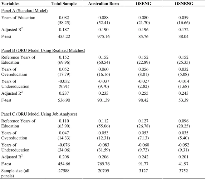
Table 2 lists selected estimated coefficients for the conventional education and experience earnings function (Panel A) and for the ORU specification (Panels B and C).10 Estimates are presented for the sample pooled across birthplace groups, and for the separate samples of the Australian born, the OSENG, and the OSNENG.
Table 2(a)
Effects of Schooling on Earnings Using Standard and ORU Models by Birthplace, Australia 2001
Variables Total Sample Australian Born OSENG OSNENG Panel A (Standard Model)
Years of Education 0.082 (58.25)
0.088 (52.41)
0.080 (21.70)
0.059 (16.66)
Adjusted R2 0.187 0.190 0.196 0.172
F-test 455.22 975.16 85.76 38.04
Panel B (ORU Model Using Realized Matches) Reference Years of
Education
0.152 (69.96)
0.152 (60.54)
0.152 (22.89)
0.152 (25.35) Years of
Overeducation
0.052 (17.79)
0.060 (16.16)
0.056 (8.01)
0.032 (5.08) Years of
Undereducation
-0.032 (9.91)
-0.037 (9.70)
-0.027 (2.82)
-0.014 (1.68)
Adjusted R2 0.237 0.233 0.255 0.243
F-test 536.90 901.39 98.42 53.39
Panel C (ORU Model Using Job Analyses) Reference Years of
Education
0.110 (63.90)
0.112 (55.06)
0.127 (26.78)
0.096 (20.25) Years of
Overeducation
0.047 (14.33)
0.053 (12.31)
0.053 (7.13)
0.035 (5.40) Years of
Undereducation
-0.076 (34.06)
-0.083 (31.59)
-0.060 (9.72)
-0.052 (9.31)
Adjusted R2 0.208 0.206 0.242 0.201
F-test 454.66 769.76 91.77 41.97
Sample size (all panels)
27588 20709 3127 3752 Source: 2001 Australian Census Household Sample File (HSF).
Note: (a) Heteroscedastic consistent ‘t’ statistics in parentheses.
10Appendix B, available from the authors upon request, reports the entire regression equations for the models of Table 2. These show that the partial effects of the non-education variables are consistent with the literature for Australia (see Miller and Neo, 2003; Chiswick and Miller, 1985; Beggs and Chapman, 1988).
The years of education variable in the conventional specification (Panel A) records the actual years of full-time education of each worker, and its coefficient indicates the return to one additional year of education. This return is 8.2 percent for the pooled sample.11 When separate analyses are conducted for birthplace groups, the Australian born have the highest return (8.8 percent) compared to the OSENG (8.0 percent) and the OSNENG (5.9 percent).12 The important feature of the results is that the payoff to schooling for the foreign born is lower than that for the native born, overall and particularly for the OSNENG. This evidence is consistent with that reported in Chiswick and Miller (2008) based on analyses of the 2000 US Census, the results in Chiswick and Miller (2009b) for the Canadian labor market (with both of these studies providing the basis for the across-country comparisons in Section VI), and also with the studies of other time periods in the US and for other countries summarised in Section I.
Panel B of Table 2 presents estimates of the coefficients of the education variables in the Over-, Required and Under-education (ORU) model based on the realized matches procedure. The inclusion of these three variables in the estimating equation has minimal impact on the estimated coefficients of any variables other than that of education. This change to the specification, however, has a marked impact on the explanatory power of the model, raising the adjusted R2 by between 4 and 7 percentage points. The largest impact is for the OSNENG regression.
The coefficients on the education variables in Panel B tell quite a different story than that contained in the conventional model of Panel A. The test that the conventional
11This rate is comparable to those reported by Preston (2001), of around 9 percent using 1981, 1991 and 1996 Australian Census data, and a simple specification of the earnings equation that contains only education and experience variables.
12 In a study of the 1981 Australian Census, Chiswick and Miller (1985) found that the estimated returns for the three birthplace groups were 8.7 percent, 8.8 percent and 4.6 percent, respectively.
specification holds was rejected by the data (i.e., that R O U , where R is the coefficient on required education, O is the coefficient on the overeducation variable and U is the coefficient on the undereducation variable).
The return to education that is correctly matched to the standards of the worker’s job is around 15 percent for each of the birthplace groups. These rates of return to education are much higher than those generated by the conventional model (see Panel A), but they are consistent with findings based on the realized matches procedure from the 2000 US Census reported in Chiswick and Miller (2008) and from the 2001 Census of Canada in Chiswick and Miller (2009b). Indeed, in the US analysis, the return to correctly matched education was also around 15 percent.
The higher value of the rate of return found with this specification of the estimating equation than with the conventional model employed in Panel A arises because account is taken of poorly matched education – that is, cases where a person has too little or too much education compared to that which is usual for their job. Moreover, the smaller effect of schooling on earnings for the OSNENG vanishes when focusing only on the return to correctly matched years of education. This suggests that the lower payoff to schooling for the foreign born is associated with different propensities for the groups to have levels of education that are “correct” for their jobs, or with wage differences associated with mismatch.
We return to this matter below.
The coefficient for the overeducation variable is positive. This implies that a worker will earn more than his counterparts for each year of education he has which is surplus to the standards of his job. For instance, if an Australian native with 11 years of education is working in a job where it is usual to have only 10 years of education, he will earn 6.0 percent
more than his counterparts with 10 years of education.13 Years of education in excess of the standards for the job are worth less in the Australian labor market than is education that is correctly matched. An alternative way of viewing these estimates is as follows. Compared to an Australian native who obtains an extra year of education that is matched to the standards for the job, a worker for whom this extra year of education is surplus to the standards for their job will reap only 6.0 percent higher earnings – or 9.2 percentage points less than the worker whose education is correctly matched. This 9.2 percentage points effect can be viewed as a wage penalty for mismatch, that is, from being in an occupation where the typical worker has less education that the worker actually has.
The return to overeducation varies across birthplace groups, being 5.6 percent for the OSENG, and a lower 3.2 percent for the OSNENG. This evidence suggests that the schooling acquired abroad by immigrants from non-English-speaking countries is less transferable to the Australian labor market than is the schooling from English-speaking developed countries.
The negative coefficient for the undereducation variable indicates a wage penalty is associated with each year of education that falls short of the standard for the job. In this case, if an Australian-born worker with 11 years of education is working in a job where it is usual to have 12 years of education, he will earn 3.7 percentage points less than his counterparts with 12 years of education.14 Contrasting the case for overeducation, this undereducated worker will actually earn more than a worker with 11 years of education who is employed in a job where it is usual to have 11 years of education. For example, an Australian-born worker who is undereducated by one year (for example, he has 11 years of education but works in a job that usually requires 12 years of education) would earn 15.2 3.7 11.5 percentage points
13 Based on US Census data, Chiswick and Miller (2008) also documented a similar rate (5.2 percent) for the native born in the United States.
14 This finding is consistent with Voon and Miller (2005) where a wage penalty of 3.1 percentage points is found to be associated with undereducation. Chiswick and Miller (2008) recorded a rate of 5.2 percentage points for the native born in the United States.
more than the worker with a correctly matched 11 years of education (that is, the worker’s job requires only 11 years of education). 15 This negative wage effect associated with undereducation differs across birthplace groups (2.7 percent and 1.4 percent for the OSENG and OSNENG, respectively). The smaller (in absolute value) effect of undereducation for immigrants from non-English-speaking countries than for immigrants from English-speaking countries is consistent with more intense selection in immigration for the former group. This is what would be expected where the labor markets and institutions in non-English-speaking countries are more dissimilar from those in Australia than is the case for immigrants from English-speaking countries.
Panel C presents the estimated coefficients of the ORU model based on the job analysis procedure.16 While the point estimates in Panel C differ from those for the realized matches procedure in Panel B, the relative magnitudes of coefficients for the ORU variables within each birthplace group are similar for both panels B and C, as are the comparisons across birthplaces. Detailed discussion is therefore not offered, other than to note that the Panel C results also support the conclusion that the schooling acquired abroad by OSNENG is less transferable to the Australian labor market than the schooling acquired abroad by OSENG. Similarly, the smaller (in absolute value) effect of the undereducation variable for
15 This earnings gain is given by the extra year of required education for the job the person holds (15.2 percent) less the wage penalty for being mismatched (3.7 percent).
16 Two alternatives for assessing the required level of education were employed. Under the first, used in Panel C of Table 2, the minima set out in the ASCO descriptions were translated into a years of formal education equivalent. In the second, the qualifications set out in the ASCO descriptions were used to assign workers to the
“correctly” matched category (or otherwise), and then the mean years of education of all correctly matched workers was used. This latter method will differ from the first approach to the extent that pathways to qualifications need not be unique. For instance, workers with Year 10, Year 11 and Year 12 education report possession of a trade qualification, and hence there will be heterogeneity in the years of full-time schooling for trades qualified workers.
OSNENG than for OSENG in Panel C is again consistent with selection being more intense for OSNENG than it is for OSENG.17
V. DECOMPOSITION OF THE DIFFERENCE IN PAYOFFS TO EDUCATION FOR BIRTHPLACE GROUPS
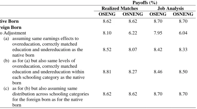
Table 3 presents the implied payoffs to schooling for both the OSENG and the OSNENG. The first two columns are based on the realized matches procedure whereas the final two columns are based on the job analysis procedure. The results for the two alternative measures are broadly the same. Hence detailed discussion is provided only for the realized matches procedure.
Table 3
Implied Payoffs to Schooling, Realized Matches and Job Analysis Procedures, Australia 2001
Payoffs (%)
Realized Matches Job Analysis OSENG OSNENG OSENG OSNENG
Native Born 8.62 8.62 8.70 8.70
Foreign Born - No Adjustment
(a) assuming same earnings effects to overeducation, correctly matched education and undereducation as the native born
(b) as for (a) but also same levels of overeducation, correctly matched education and undereducation within each schooling category as the native born
(c) as for (b) but also assuming same distribution across schooling categories for the foreign born as for the native born
8.10
8.52
8.81
8.62
6.22
8.07
8.27
8.62
7.95
8.42
8.46
8.70
6.04
8.33
8.50
8.70
17The comparisons between Panels B and C are consistent with Hartog’s (2000, p.135) conclusion that the general findings from application of the ORU model are not sensitive to the measure of required education.
Chiswick and Miller (2009a) arrive at the same conclusion in their more recent analysis.
The information for the decomposition based on the realized matches procedure listed in Table 3 shows that four-fifths of the small difference (of one-half of one percentage point) in the payoffs to schooling for the OSENG and the Australian born can be linked back to differences between the partial effects on earnings associated with either correctly matched education or mismatched education for these groups.18 As the partial earnings effects associated with correctly matched education are the same for the two groups (15.2 percent for the Australian born and for the OSENG), it is apparent that it is mismatched education that is driving the results. The differences in the earnings effects associated with overeducation and undereducation for the Australian born and the OSENG are about the same (see Panel B of Table 2), and the years of overeducation and undereducation are similar, implying that overeducation and undereducation will be approximately equal contributors to this part of the decomposition. This is confirmed by tests, where the predicted earnings for each category of education were formed replacing the earnings effects and means for the ORU variables one- by-one, rather than as a set.
In the case of the OSNENG, 77 percent of the difference in the payoffs to education for this group and the Australian born (of 2.4 percentage points) is explained by the differences between the partial earnings effects associated with overeducation and undereducation.19 About another 8 percent is due to the differences in distributions of workers across overeducation/undereducation categories within each educational category.20 Lastly,
18 That is, 8.52 8.10 8.62 8.10 0.81
.
19 That is, 8.07 6.22 0.77.
8.62 6.22
20 That is, 8.27 8.07 0.08.
8.62 6.22
approximately 15 percent of the gap is caused by the different representations of this group of foreign born and the Australian born across the education categories.21
The differences in the partial earnings effects between the foreign born and native born associated with undereducation are attributed in Chiswick and Miller (2008) to the
“unobserved” attributes of immigrants that permit them to compete successfully for jobs for which they are under-qualified, in terms of formal schooling. Higher levels of motivation, decision making skills, and innate ability are the main possibilities that have been raised in the literature. The difference in the partial earnings effects associated with overeducation most likely are associated with the non-recognition of overseas qualifications (whether formal or informal) because skills are not fully transferable.22
These findings mirror reasonably well the results of the decompositions for the US provided by Chiswick and Miller (2008), where most of the difference in the payoffs to schooling between immigrants from non-English-speaking countries and the native born can be linked to the earnings effects associated with overeducation and undereducation.
Finally, the broad similarity of the findings in Table 3 based on the realized matches and job analysis procedures is to be noted. Thus, the Chiswick-Miller decomposition does not appear to be sensitive to the measurement of the usual level of education for occupations in the Australian labor market.
21 That is, 8.62 8.27 0.15.
8.62 6.22
22An alternative that has been raised in the literature (e.g., Miller and Neo (2003), drawing on Greeley (1976)) is that the labor market is characterised by a subtle form of discrimination that is more intense among the better educated. Another alternative is lower quality of foreign schooling. These explanation, however, are not consistent with the similarity of the estimated payoffs for the foreign born and native born to years of education that match the requirements of the workers’ jobs.
VI. INTERNATIONAL COMPARISONS
Analyses similar to those presented here have recently been undertaken for the US (Chiswick and Miller, 2008) and Canada (Chiswick and Miller, 2009b). In the US immigration is dominated by family reunification, with skill-tested visas playing a minor role.
In 2007, for example, 17.7 percent of (non-refugee) immigrants to the US entered under employment preference visas, including the visas provided to the accompanying spouse and minor children of the skill-tested applicant. In the same year, 66.5 percent of non-refugee immigrants to Canada were categorized as “economic immigrants”. In 2007-2008, 68.4 percent of non-refugee immigrants to Australia entered under skilled (points-tested) visas.
A summary of the results from application of the Chiswick and Miller (2008) decomposition to data for Australia, Canada and the US is presented in Table 4.
In Australia, Canada and the US, adjustment for the means of the ORU variables has little impact on the implied payoff to schooling. Adjustment for the different distributions of the foreign born and native born across the educational categories has minimal impact on the implied payoff to schooling in Canada and Australia, but it has a reasonably important effect in the US, particularly among immigrants from less-developed countries. This is the Latino effect that Antecol et al. (2003) have previously noted as being important in comparisons involving these three countries. The larger part of the gap between the payoff to schooling for immigrants and the native born in each country, however, is linked to differences in the earnings effects of the ORU variables. In Australia, these earnings effects account for around 80 percent of the payoff differential, for both OSENG and OSNENG. In Canada the figure is 88 percent, whereas in the US the figure is 76 percent for immigrants from developed countries, and 62 percent for immigrants from less-developed countries.
Table 4
Cross-Country Comparison of Decomposition of Immigrant/Native-Born Difference in Payoff to Education, Males, Australia, Canada and the US
Country
Payoff:
Native Born
Payoff:
Foreign Born
Payoff: Foreign Born Adjusting for Estimated
ORU Effects
Payoff: Foreign Born Adjusting for Means of ORU Variables
Payoff:
Foreign Born Adjusting for
Weights
Australia-OSENG 8.6 8.1 8.5 8.8 8.6
Australia-OSNENG 8.6 6.2 8.1 8.3 8.6
Canada 7.6 6.0 7.4 7.5 7.6
US-Total 10.5 5.3 8.5 8.6 10.5
US-Developed 10.5 7.1 9.7 9.9 10.5
US-LDC 10.5 4.7 8.3 8.5 10.5
Source: Table 3 of this paper, Tables 6 and 8 of Chiswick and Miller (2008), Table 4 of Chiswick and Miller (2009b).
In Australia, which arguably has the tightest points-testing, the earnings effects of undereducation and overeducation make approximately equal contributions to the earnings effects component of the gap between the payoffs to schooling for the native born and the foreign born. In Canada, the calculations presented in Chiswick and Miller (2009b) show that the earnings effects of undereducation are about twice as important as the earnings effects of overeducation. In the US, however, the earnings effects of undereducation are fully ten times more important than the earnings effects of overeducation. In other words, as the importance of visas issued on the basis of family ties increases relative to selection based on skill testing by migration authorities, the role of undereducation, which is more prevalent among low- skilled workers, also increases. Concomitantly, a greater role for skill-based visas by immigration authorities appears to result in overeducation. Overeducation is associated with the limited international transferability of the human capital immigrants acquired abroad.
Thus, the earnings patterns and the effects of schooling on the earnings of immigrants compared to natives is influenced by immigration policy.
VII. CONCLUSION
This paper has studied the earnings consequences of overeducation/undereducation in the Australian labor market among immigrants and those born in Australia using data from the 2001 Census of Population and Housing. The empirical analyses are generated using both the realized matches and job analysis procedures, and have focused on enhancing understanding of the immigrant labor market experience in Australia.
The inclusion of ORU variables in the earnings equation improved its explanatory power by up to 7 percentage points (or, equivalently, improved the degree of explanation of the earnings function by up to 40 percent), which suggests there is considerable information content to the approach. The payoff to usual levels of education for the Australian born is 15.2 percent using the realized matches procedure and 11.2 percent using the job analysis procedure. Both are much higher than the payoff obtained when the conventional schooling model using actual education is employed (8.8 percent for the Australian born).
Among immigrants from the English-speaking developed countries (OSENG), the coefficient on actual schooling is 8.0 percent, and for the usual or reference level of schooling it is 15.2 percent under the realized matches technique, and 12.7 percent under the job analysis technique. In contrast, for immigrants from other countries (OSNENG), the coefficient on actual schooling is smaller, only 5.9 percent, and for the usual level of schooling it is also 15.2 percent using realized matches and 9.6 percent for the job analysis method. Remarkably, for analyses for the US, the coefficient on usual schooling is also 15 percent for natives and immigrants using the realized matches method (Chiswick and Miller, 2008).
With each of the methods for measuring correctly matched education, there are substantial earnings effects associated with undereducation and overeducation. The wage effects associated with mismatched education vary across birthplace groups. For the OSENG, years of overeducation and of undereducation are associated with wage effects of 5.6 percent
and 2.7 percent, respectively. These wage effects are at the smaller rates of 3.2 percent and
1.4 percent, respectively, for the OSNENG. This is similar to the pattern of wage effects associated with the job analysis approach. The general conclusions on the wage effects of overeducation and undereducation in the immigrant labor market therefore do not appear to be sensitive to the choice of method for constructing these variables. The differences between the OSENG and OSNENG in the wage effects is consistent with the conventional wisdom on the relative importance of the less-than-perfect international transferability of immigrants human capital and self-selection in immigration for these two birthplace groups.
Application of the Chiswick-Miller (2008) decomposition shows that the categorization of education into its usual, overeducation and undereducation components can enhance understanding of the reasons for the lower payoff to schooling for the OSNENG.
Most of the gap (around four-fifths) between the payoff to schooling for this group of immigrants and the native born in Australia can be linked to differences in the wage effects of overeducation and undereducation. In turn, these differences in wage effects appear to be linked to the role of unobservables in the positive self selection of immigrants in the case of undereducation, and to the limited international transferability of overseas schooling in the case of overeducation. The decomposition provides a means of quantifying the importance of self-selection among the less-well qualified, and of non-recognition of foreign qualifications among those with more schooling. It also appears to debunk the myth that discrimination in the labor market is more intense against the better educated immigrants. These are important findings for the immigrant labor market in Australia, and they have clear parallels in the findings reported for the US labor market by Chiswick and Miller (2008) and the Canadian labor market by Chiswick and Miller (2009b).
The analyses show that the lower payoff to schooling for the “undereducated” can be linked to their higher earnings, ceteris paribus, that is, to positive self-selection in migration, and should not be a cause for concern among policy makers.
The favorable self-selection of immigrants (predominantly the US case) and institutional (legislated and administrative) selection (the Australian and Canadian situations) appear to generate different mixes of immigrants in terms of unobservables among the less- well educated. The policy concern regarding the lower payoff to schooling for the foreign born needs to focus only on the workers who are overeducated. Oddly enough, the relative contribution that overeducation makes to the gap in the payoff to schooling between the foreign born and native born is greater in Australia than in the US. The more stringent testing of immigrants for entry into Australia does not appear to be accompanied by improved international transferability of the skills immigrants acquired abroad. Because of the favorable selectivity of immigrants, even if the issues associated with the limited international transferability of schooling acquired abroad can be addressed, the payoff to schooling for the OSNENG will still fall short of that for the native born. Elsewhere (Chiswick and Miller, 2009c), it is shown that the degree of overeducation diminishes with duration in the destination as immigrants adjust their occupations to better match their educational qualifications. Policies to facilitate this process are worthy of consideration.
APPENDIX A
DEFINITIONS OF VARIABLES
The variables used in the statistical analysis of the 2001 Australian Census of Population and Housing are defined below. The analyses are restricted to male full-time workers (i.e., working 35 hours or more per week) aged 20-64 years.
Dependent Variables
Log of Hourly Earnings Natural logarithm of hourly earnings (where earnings are defined as gross earnings from all sources). As weekly earnings were coded in intervals, midpoints of intervals were used to construct a continuous measure. The open-ended upper category was assigned a value of 1.5 times the lower threshold level. Weekly hours were recorded in intervals so midpoints were used to construct a continuous measure. Hourly earnings was then constructed by dividing weekly earnings by weekly hours worked.
Explanatory Variables
Years of Education This is a continuous variable that records the equivalent years of full-time education completed by the individual. Those holding a Postgraduate degree are assigned 19 years of education, Graduate Diploma and Graduate Certificate holders are assumed to have 17 years, Bachelor degree holders have the equivalent of 15.5 years of education, Advanced Diploma and Diploma holders are coded as having 14 years, holders of Certificates are assigned 13 years, those who have completed either Year 9 or any years through to Year 12 are coded as 9, 10, 11 and 12 years of education, respectively, and those who did not go to school or attained Year 8 or below are assumed to have 7 years of education.
Reference Education (YRIGHT)
This variable records “correctly matched” years of education.
It is constructed using the mean level of education in the occupation of employment for the Realized Matches procedure. For the Job Analysis procedure, the minimum required level of education for each occupation was obtained from the Australian Standard Classification of Occupations.
Further details are given in the text.
Overeducation (YOVER)
The overeducation variable equals the difference between the person’s actual years of education and the years of education required for the person’s job where this computation is positive. Otherwise, it is set equal to zero.
Undereducation (YUNDER)
The undereducation variable equals the difference between the years of education required for the person’s job and the person’s actual years of education where this computation is positive. Otherwise, it is set equal to zero.
Age This is a continuous variable for age.
Marital Status Binary variable set to one if an individual is married and set to
zero otherwise.
Birthplace of individual Two dummy variables were constructed for individuals who were born overseas (OSENG for overseas born from English- speaking developed countries; OSNENG for overseas born from non-English-speaking countries). Both are set equal to one for the respective groups of foreign born and zero otherwise. Birthplaces for the Foreign Born are: New Zealand (benchmark region for OSENG), Other English Speaking Developed Countries, Europe (benchmark region for OSNENG), South Eastern Europe, Africa, Middle East and North Africa, South East Asia, China, Southern and Central Asia, Pacific Islands, Japan and Korea, and Latin America.
Duration of Residence in Australia
This records the number of years an individual born overseas has lived in Australia. Three dummy variables were created based on the Census information: Arrived 1991-1995, Arrived 1986-1990, Arrived before 1986. The benchmark group is those who arrived after 1995.
Experience The experience variable was derived using the Mincer (1974) Proxy; Age – Years of Education – 5.
Government Employment
This is binary variable that distinguish between those working in government organizations and those working in the private sector.
Table A.1
Descriptive Statistics for Variables in the Models of Earnings Determination, Australia 2001
Variables Total Sample
Australian Born
Overseas Born English-Speaking Countries (OSENG)
Overseas Born non- English-Speaking Countries (OSNENG)
Log Earnings 2.896
(0.56)
2.882 (0.56)
3.004 (0.54)
2.883 (0.56) Actual Years of
Education
12.213 (2.52)
12.072 (2.40)
12.594 (2.49)
12.673 (3.07) Reference Years of
Education(a)
12.144 (1.44)
12.109 (1.42)
12.356 (1.46)
12.159 (1.53) Years of
Overeducation(a)
0.801 (1.28)
0.704 (1.17)
0.907 (1.37)
1.251 (1.61) Years of
Undereducation(a)
0.732 (1.15)
0.740 (1.13)
0.670 (1.07)
0.737 (1.30) Years of Experience
(EXPER)
22.626 (11.52)
21.761 (11.50)
25.430 (10.75)
25.066 (11.47) Married 0.727
(0.45)
0.708 (0.45)
0.79 (0.41)
0.780 (0.41) Government
Employment
0.157 (0.36)
0.164 (0.37)
0.151 (0.36)
0.124 (0.33) Speaks English Very
Well
0.093 (0.29)
(b) (b) 0.408
(0.49) Speaks English Well 0.034
(0.18)
(b) (b) 0.231
(0.42) Speaks English Not
Well
0.010 (0.101)
(b) (b) 0.072
(0.26) Speaks English Not at
All
0.001 (0.02)
(b) (b) 0.004
(0.06) OSENG 0.113
(0.317)
(b) (b) (b)
OSNENG 0.136 (0.343)
(b) (b) (b)
New Zealand (b) (b) 0.245
(0.43)
(b) Other English
Speaking Developed Countries
(b) (b) 0.755
(0.43)
(b)
Europe (b) (b) (b) 0.274
(0.45)
South Eastern Europe (b) (b) (b) 0.124
(0.33)
Africa (b) (b) (b) 0.032
(0.18) Middle East and North
Africa
(b) (b) (b) 0.089
(0.29)
South East Asia (b) (b) (b) 0.193
(0.39)
China (b) (b) (b) 0.086
(0.28) Southern and Central
Asia
(b) (b) (b) 0.101
(0.30)
Pacific Islands (b) (b) (b) 0.042
(0.20)
Japan and Korea (b) (b) (b) 0.018
(0.13)
Latin America (b) (b) (b) 0.041
(0.20) Arrived after 1995 0.031
(0.17)
(b) 0.145
(0.35)
0.104 (0.31) Arrived 1991-1995 0.022
(0.15)
(b) 0.068
(0.25)
0.107 (0.31) Arrived 1986-1990 0.039
(0.19)
(b) 0.125
(0.33)
0.183 (0.39) Arrived Before 1986 0.157
(0.36)
(b) 0.661
(0.47)
0.606 (0.49) Source: 2001 Australian Census Household Sample File (HSF).
Notes: Table lists the means and standard deviations (in parentheses).
(a) = Based on realized matches procedure.
(b) = Variable not relevant.