Modeling Assessments of Climate Engineering

(1)

i

Modeling Assessments of Climate Engineering

Dissertation zur Erlangung des Doktorgrades der Mathematsch-Naturwissenshaftlichen Falkutät

der Christian-Albrechts-Universität zu Kiel

vorgelgt von Yuming Feng Kiel, Dezember 2016

(2)

ii Referent: Prof. Dr. Andreas Oschlies

Korreferent #1: Prof. Dr. Martin Visbeck Tag der mündlich Prüfung: 2017-02-15

(3)

iii

Summary

Climate Engineering (CE), defined as the deliberate intervention in the Earth’s climate system in large scale to alleviate global warming, has been discussed as an important option to counter climate change challenges. In this thesis, I conducted five assessments on some specific CE technologies using the University of Victoria Earth System Climate Model (UVic_ESCM).

Each individual assessment investigated the climate responses when particular CE technologies were applied under high CO² emission scenarios from year 2020 to 2099. The main aim of those assessments is to improve the understanding of CE technologies regarding their global warming offset efficacy, environmental side effects, simulation uncertainties, and extended usages potentially.

Artificial Ocean Alkalinization (AOA), which could remove carbon dioxide from atmosphere by artificially dissolving alkaline minerals (e.g. lime and olivine), was the focus for the first two assessments. In the first assessment, implementing lime-based AOA in Barrier Reef, Caribbean Sea and South China Sea, was tested effective for protecting local coral habitat from ocean acidification threats. However a rapid rebound to the acidified conditions of the experimental regions was observed if AOA was stopped. The second assessment studied the climate responses when olivine-based AOA was implemented along the ice-free coastal waters.

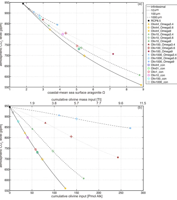
Decreasing olivine grain diameter from 1000 to 10 µm could provide a higher overall CO² sequestration efficiency despite the fact that grinding smaller olivine grains could emit more CO². If some aragonite Ω upper limits were taken to prevent excessive alkalinization from harming the

(4)

iv

marine ecosystems, AOA in coastal waters could still reduce atmospheric CO² by 89.4~595.56 GtC cumulatively by year 2100.

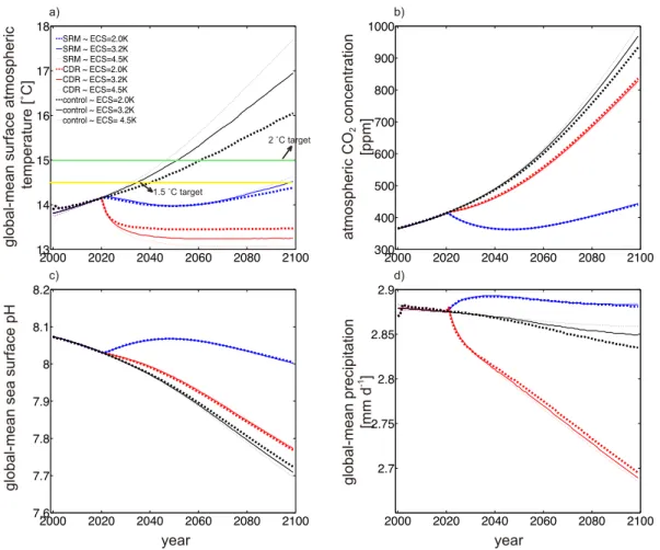
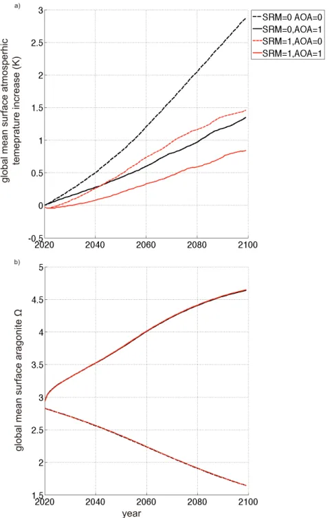
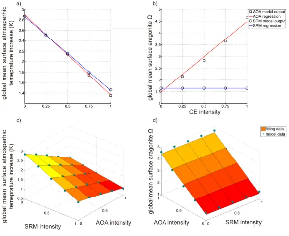
In the third assessment, sulphate aerosol injection-based SRM, and direct air capture- based CDR, were evaluated under different equilibrium climate sensitivities (ECSs) as well as CE intensities separately. Under the same CE intensities, SRM and CDR induced global-mean surface temperature reductions from respective control run levels in year 2099, were larger if ECS was set higher. While under higher ECS, more SRM and CDR were required than the case under lower ECS, if they were employed for stopping >1.5 °C global warming from the preindustrial in 21st century. For the studied cases, the climate feedback caused cooling were 14%~52% and 45%~86% in magnitude to that from direct SRM and CDR radiative perturbations. Preliminary results from the forth assessment found that to prevent global warming and ocean acidification concurrently, combining lime-based AOA with sulphate aerosol injection-based SRM had some economic advances compared to implementing it alone, but the marginal costs for this approach would increase dramatically due to the nonlinearity interactions generated within those combined schemes.

The last assessment was a comprehensive study that compares the climate mitigation effectiveness and side effects of Afforestation, Artificial Ocean Upwelling, Ocean Iron Fertilization, AOA, and SRM. As a summary, the results showed those CE technologies were either not effective enough for mitigating the global warming obviously, or potentially having some severe environmental side effects.

(5)

v

Zusammenfassung

Climate Engineering (CE) wird als eine gezielte großskalige Intervention ins Erd- und Klimasystem definiert, um die globale Erwärmung und die damit verbundenen Klimaauswirkungen zu verringern. Es wird schon als wichtige Alternative zur Bewältigung der Klimaveränderung gesehen. In dieser Arbeit habe ich mit dem University of Victoria Earth System Climate Model (UVic_ESCM) fünf Evaluierungen zu einigen vorhandenen CE- Technologien durchgeführt. Jede einzelne Evaluierung untersucht die Reaktion des Klimas, wenn eine oder mehrere CE-Technologien unter besonderen CO²-Emissionsszenarien von 2020 bis 2099 eingesetzt wurden. Das Hauptziel dieser Evaluierungen ist, das Verständnis für die Effektivität der Reduzierung der globalen Erwärmung, umweltbedingte Nebenwirkungen, Simulationsunsicherheiten und potenzielle Anwendungen der spezifischen CE-Technologien zu verbessern.

Artificial Ocean Alkalinization (AOA) war der Schwerpunkt der ersten beiden Evaluierungen, was das CO² aus der Atmosphäre durch künstliche Auflösung von alkalischen Mineralien (z. B.

Calciumoxid und Olivin) entfernen könnte. In der ersten Evaluierung wurde nachgewiesen, dass die Umsetzung der zeitbasierten AOA in Great Barrier Reef, Caribbean Sea and South China Sea ein wirksamer Ansatz ist, den lokalen Korallenlebensraum vor den Bedrohungen der Ozeanversauerung schützen zu können. Allerdings existiert ein schneller Rückgang zu den angesäuerten Bedingungen der Zielregionen, wenn die Anwendung der AOA beendet wird. Die zweite Evaluierung schätzte das erzielte Klimaschutzpotenzial, als olivinbasierte AOA entlang

(6)

vi

der eisfreien Küstengewässer angewandt wurde. Es gab eine rasch erhöhte Klimaschutzeffizienz, wenn kleinere Olivinkörner sogar unter Berücksichtigung des Mahlprozesses verwendet wurden, der mit der CO²-Kompensation in Zusammenhang steht. Im Allgemeinen hatte AOA in den Küstengewässern Klimaschutzpotenziale, obwohl die Aragonit-Ω-Obergrenze genommen wurde, um übermäßige Alkalisierung zu vermeiden, die die Meeresökosysteme schädigen könnte.

Die dritte und die vierte Evaluierung untersuchten zwei verschiedene CE-Technologien. In der dritten Evaluierung werden auf der Einspritzung der Sulfatsaerosol-basierten SRM und auf der Basis von direkter Erfassung der Luft stehenden CDR unter verschiedenen Gleichgewichts- Klimasensitivitäten (equilibrium climate sensitivities, ECS) und Ingenieurintensitäten analysiert.

Der Stand der Temperatursenkung der globalen Oberfläche, der durch ausgewerteter CE- Technologie verursacht war und mit der Referenz verglichen wurde, war umso größer, je größer ECS war. In diesem Fall wurden jedoch mehr SRM und CDR benötigt, um die globale Erwärmung auf nicht mehr als 1.5 ° C im 21. Jahrhundert effektiv zu beschränken. Erste Ergebnisse aus der vierten Evaluierung zeigten, um die gleichen Klimaschutzziele – das gleichzeitige Vorkommen der globalen Erwärmung und Ozeanversauerung zu vermeiden - zu erreichen, hat die Kombination von calciumoxidbasiertem AOA mit auf der Einspritzung der Sulfatsaerosol basierten SRM einen wirtschaftlichen Vorteil als einzelne Umsetzung, aber die negativen Externalitäten wie Niederschlagsanomalien könnten bleiben.

Die letzte Evaluierung war eine Synthese-Studie, die die Wirksamkeit der Effekte des Klimaschutzes und Nebenwirkungen von Aufforstung, künstlichem Ozeanauftrieb,

(7)

vii

Ozeaneisendüngung, Ozeanalkalinisierung und Solar Radiation Management (SRM) vergleicht.

Jedoch zeigten die Ergebnisse, dass die CE-Technologien entweder nicht wirksam genug waren, um die globale Erwärmung zu reduzieren, oder potenziell einige starke Nebenwirkungen hatten.

(8)

viii

1. Introduction

1.1. Climate Engineering Concepts

Climate change is considered one of the biggest threats to mankind in the 21^st century. The Intergovernmental Panel on Climate Change (IPCC 2014) shows that the global average temperature has a linear trend of warming with 0.85 °C (IPCC- WG1 2013) since 1880 to 2012. The unequivocal concept of climate change is associated with impacts such as sea level rise, ocean acidification, oceanic oxygen decrease and extreme weather conditions, etc. The climate change caused by anthropogenic green house gas (GHG) emissions begins to result in severe consequences, for both human society and biodiversity (Figure 1-1).

For the future, numerical climate models have demonstrated a continued surface temperature increase (Figure 1-1) if GHG emissions keep on. The temperature will exceed 1.5 °C by 2100 under medium and high emission pressure (IPCC-WG1 2013). Continued climate change will amplify the current risks for urban and natural ecosystems, and some of the associated impacts, such as ocean acidification, can still last for several centuries after surface temperature stabilization.

Therefore measures such as climate adaptation and mitigation, are required to prevent the above-mentioned pervasive consequences from happening (IPCC-WG2 2014).

(13)

Figure 1-1. The environmental risks from climate change and their relationship to global-mean surface temperature change (referenced to preindustrial level) (a), cumulative anthropogenic CO² emissions (counted from year 1870) (b) and global GHG emission changes between year 2050 to 2010 (c). The results are based on Coupled Model Intercomparison Project Phase 5 (CMIP5) simulations (pink plume in Panel (b)) and on a simple climate model for the baselines and five mitigation scenarios (colored ellipses). This figure is achieved and modified from IPCC-WG1 (2013).

Climate adaptation is the process of adjustment to avoid the direct harmful climate impacts, while climate mitigation refers to technologies that can reduce or prevent GHG emissions. Climate adaption is considered essential, but it has limited effectiveness if the rate of climate change is high. Climate mitigation measures can ideally reduce emissions close to zero, and therefore diminish the climate change

(14)

risks. An example of such climate mitigation technology is the carbon capture and storage (CCS). CCS captures waste carbon dioxide from large point sources (e.g.

industrial sectors) and deposits it in geological formations resulting in overall CO² emission declines. However to massively reduce anthropogenic CO² concentrations in 21^st century via climate mitigation technologies alone, humanity will require intensive global industrial reformations (Figure 1-2). This large-scaled reformation can be very difficult to fully commit to due to the industrial inertia and short time window left to avert harmful climate change impacts.

Figure 1-2. Atmospheric GHG emissions (as CO² equivalent) under different future GHG scenarios (a) and associated scale-up requirements for low-carbon energy sources for year 2030, 2050 and 2100, compared to the level in 2010 (b).

Figure is from IPCC-WG2 (2014).

(15)

Besides climate adaptation and mitigation, a potential alternative to deal with climate change is climate engineering (CE, also named geoengineering). CE is the process that is designed to deliberately alter the climate system on a large scale for alleviating climate change impacts. In specific, most CE technologies can be categorized into either “Solar Radiation Management” (SRM) branch, which aims to reduce incoming solar radiation, or “Carbon Dioxide Removal” (CDR) branch, which operates by enriching terrestrial and oceanic carbon reservoirs (Figure 1-3). This categorization is not given according to a CE technology’s climate affects. Whether a CE technology should be considered as SRM or CDR, depends on if it primarily deals with the cause or the consequence of anthropogenic climate change. If the primary aim of a CE technology is to mitigate the continuously increased atmospheric CO², i.e.

the cause of climate change, this CE technology usually belongs to CDR branch. In contrast, if a CE technology in the first place aims to offset the increase of surface temperature, i.e. the consequence of climate change, via solar insolation reduction, this technology is usually considered SRM.

Though CE is brought up apart from climate mitigation in previous paragraphs, it has some overlaps with climate mitigation. Since CDR can decrease the atmospheric CO², it is a particular climate mitigation technology by definition.

Albeit several CDR technologies such as Reforestation (RFO) have been included in some mitigation scenarios (e.g. Representative Concentration Pathway 2.6), most CE methods (mainly SRM methods) have not yet been involved. In the CE research community, “geoengineering“ in early studies is widely used to describe SRM technologies. In some particular contexts, climate mitigation refers to any effort that

(16)

can decrease the global warming rate other than the atmospheric CO²elevation.

Upon this definition, SRM, which has weak intervention to carbon cycle, can also be regarded as climate mitigation technology. To avoid those terminological complexities, “climate mitigation” used in this chapter is defined as the measures to decrease atmospheric CO² concentrations.

1.2. Climate Engineering History

Since the industrial revolution, the first idea to modify the weather and climate for serving humanity came from American Meteorologist James Pollard Espy, who introduced a method of setting fires to generate precipitation on command in year 1841. In the middle of the 20st century, the Soviet and the United States government both established their institutes to study “cloud seeding” to alter the weather. During the Vietnam War, the US air force deployed cloud seeding operations as a hostile weather manipulation for the first time. Learning from the history of Vietnam War, the United Nations general assembly later approved the Environmental Modification Convention (EMC) that was ratified by 76 countries for banning the wartime and other hostile use of modifying weather and climate. In 1974, Russian scientist Mikhail Budyko brought up the idea of burning sulfur and sending these aerosols in the stratosphere to reverse global warming. Following his proposal the concept of “Solar Radiation Management” is gradually formed and became one of the two major study branches of CE (Keith 2000). During the cold war, the concerns of nuclear war eventually formed the theory of “nuclear winter”. In nuclear warfare scenarios, the firestorms caused by massive nuclear bomb explosions could generate a huge aerosol/dust shield to reflect solar radiation for years and

(17)

reverse anthropogenic global warming effects (Robock 1984). The catastrophic consequence of nuclear winter was compared to Cretaceous-Paleogene (K-Pg) extinction event. One popular hypothesis for this event suggests this extinction is due to the Earth cooling effect caused by planetary albedo enhancement from massive volcanism and firestorm during the Chicxulub Asteroid impact (Pope et al.

1998). In 1991, Mount Pinatubo erupted and threw millions of tons of volcanic ashes into the atmosphere and reduced the global-mean surface temperature by 0.5 °C in the following two years (McCormick et al. 1995). This natural phenomenon is often considered as an analogue to implementing SRM. In 2006, Nobel Prizer Paul Crutzen advocated for promoting SRM related research (Crutzen 2006), which triggered a new bloom for SRM study till nowadays.

The earliest work on CDR was traced back to the 1970s in the US Department of Energy. After 1970s, the idea of planting tress to remove CO² from atmosphere began to occur. In 1977, Marchetti proposed to scrub CO² from smoke stacks and inject the stream into Mediterranean outflow water as a prototype to capture CO² from both atmosphere (CDR) and industrial exhaust (CCS). In 1992, the First International Conference on Carbon Dioxide Removal (ICCDR-1) was held in Amsterdam, representing the first major gathering of researchers in the field of CO² capture, disposal and utilization (Blok et al. 1992). Thereafter the CDR branch was gradually established.

After 2010, due to the urgency of dealing with climate change and the potential CE, several strategic projects designed to study CE were initiated in UK (Royal Society 2009, Pidgeon et al. 2013), USA (NAS 2015), Germany (Rickels et al.

(18)

2011) and China (Cao et al. 2015). In 2011, an IPCC expert meeting on climate engineering was held in Lima, Peru (Edenhofer et al. 2011). In 2014, IPCC in its fifth assessment began to discuss CE options (IPCC-WG1 2013).

Figure 1-3. Illustration for commonly discussed CE technologies. Figure Source:

Rickels et al. (2011).

Due to the complexity and uncertainties of climate system as well as CE technologies, implementing CE in present world, is expensive and will likely lead to some environmental side effects. Therefore scientists tend to use climate models to study CE technologies upon their environmental and social-economical impacts. The past several years have witnessed a great improvement in our understanding of CE.

In following paragraphs I will examine some of the most discussed CE technologies in specific and give a brief literature review of the relevant studies.

(19)

1.2. Solar Radiation Management 1.2.1. Stratospheric Aerosol Injection

SRM has been suggested as a policy response to avert some of the most severe impacts of anthropogenic global warming (Crutzen 2006). Stratospheric aerosol injection (SAI), the most frequently discussed method of SRM, involves injection of sulfur dioxide (SO2) into the tropical stratosphere to raise the planetary albedo. It reduces insolation in an attempt to offset some fraction of anthropogenic warming. The meridional circulation of the stratosphere is mainly governed by vast regions of upwelling in the tropics and large-scale sinking in the extratropics. SO² injections into the tropical stratosphere will mix well globally within weeks through this Brewer-Dobson circulation, resulting with a relatively homogeneous stratosphere (Bala et al. 2003).

Climate models with comprehensive atmosphere dynamics and chemistry can simulate a stratospheric aerosol layer in several ways, including by direct injection of sulfates into the stratosphere or a prescribed aerosol layer (Kravitz et al.

2011). However, many modeling groups choose to simply dim the sun by changing the solar constant in a climate model. This simpler design is often used because solar dimming may be easier to implement than SAI in coding aspects. In many cases, it allows modelers to study the effects of reduced insolation even if the model is incapable to simulate complex dynamical changes induced by SAI. One large difference between SAI simulations and solar dimming simulations is the perturbation over the circulation near the Southern Ocean. Stratospheric heating triggered by SAI is not seen in solar dimming simulations. SAI simulations induce a

(20)

large equator to pole temperature gradient in the stratosphere, strengthening the Jetstream and high-latitude surface winds. This anomalous wind stress applied to the ocean allows for greater mixing in the Southern Ocean, and subsequently promotes warm advection of water toward the Antarctic ice-sheets (McCusker et al.

2015). In addition, solar dimming cannot be used to simulate the changes in atmospheric chemistry triggered by SAI. Those different model designs are summarized Geoengineering Model Intercomparison Project (GeoMIP) (Kravitz et al.

2011), in which solar dimming design is presented in the G1 (solar dimming deployed to compensate instantaneous 4xCO² increase) and G2 (solar dimming deployed to compensate 1% yr^-1 CO² increase) Groups while SAI is set in G3 (SAI deployed to compensate CO²forcing following RCP 4.5 scenario) and G4 (SAI deployed in constant rates per year) Groups. Therefore, while solar dimming is often a good approximation of an SAI engineered climate, the difference may become significant when discussing particular elements of the climate response to SAI.

A major concern associated with SAI is the perturbation over global hydrological cycles. Globally, the precipitation under SAI is reduced compared to the case without it (Tilmes et al. 2013). According to an SAI model comparison study (Kravitz et al. 2013a), global precipitation is reduced by around 4.5% once radiative forcing rebounds to preindustrial level by SAI under quadrupled CO² condition using solar dimming approach. Kleidon et al. (2015) found that much of the global- scale change in the hydrologic cycle can be robustly predicted by the response of the thermodynamically constrained surface energy balance to altered radiative forcing.

Bala et al. (2008) found that SAI could not offset temperature elevation and

(21)

hydrological perturbation under climate change at once, because insolation change by SAI can directly perturb both the surface latent and sensible heat flux. Kravitz et al.

(2013b) figured out the SAI runs have a smaller magnitude of land sensible but larger latent heat flux adjustments than the control run, which implies a greater reduction of evaporation and less land temperature increase induced by SAI.

SAI can also perturb the cloud and associated thermal dynamics in atmosphere. Besides the mentioned perturbation on circulation over Southern Ocean, English et al. (2012) found simulated SAI in tropical atmosphere will result a significant perturbation to tropospheric aerosols with enhanced sulfate burden particularly in upper layer and near poles. There is also evidence indicating that SAI will change the pattern of extreme weathers in global patterns and frequencies (Curry et al. 2014). When SAI is terminated abruptly while atmospheric CO² level is still high, the global-mean precipitation rate is increased (Matthews and Caldeira 2007), while mitigated global-mean temperature (Jones et al. 2013) will rebound to unmitigated level in less than several years.

SAI can also affect the global biogeochemical cycles. Studies (Tilmes et al.

2008, Tilmes et al. 2012 and Heckendorn et al. 2011) found sulphate aerosols can accelerate the hydroxyl catalyzed ozone destruction and caused a rapid depletion even though future halogen concentration will be much reduced. Carbon changes are often observed in SRM engineered future. Matthews and Caldeira (2007) using a climate model with fully coupled carbon cycle found SAI could enhance the terrestrial and ocean carbon uptake compared with the control run. Some other

(22)

research also confirmed that land carbon sinks will be enhanced through increasing diffuse solar radiation (Mercado et al. 2009, Xia et al. 2016).

While many studies show that SRM would be effective in reducing global- mean temperature, there are likely disparate regional impacts. Yu et al. (2015) and Jones et al. (2010) looked into the temperature and precipitation compensation inequalities under SAI and found those inequalities vary greatly from one region to another. Ricke et al. (2011) found that when SAI is used in an attempt to reduce the rate of increase in surface air temperature, the effectiveness of the SAI in stabilizing regional climates decreases if climate sensitivity is higher.

Some studies investigated the socioeconomic impacts induced by SAI. SAI itself has been long considered inexpensive (Barrett 2008). McClellan et al. (2012) concluded that the engineering price to implement SAI to effectively mitigate climate change is less than 8 billion USD per year. However, Klepper and Rickels (2012) pointed out that price and external effects are not yet sufficiently accounted for, and that the question of dynamic efficiency is still unresolved.

More recently, some scientists began to focus on improving the implementation strategies to enhance SAI’s efficiency to reduce global warming to avoid harmful environmental side effects and to diminish the involved uncertainties.

Keith and MacMartin (2015) pointed that the environmental impacts of SAI are largely depending on the implementation scenario, and the negative externality is not SAI’s inherent feature. MacMartin et al. (2014) suggested only implementing SAI for constraining the rate of global-mean temperature change instead of atmospheric CO² forcing change. It will lead to a finite deployment period depending on

(23)

emission pathway. Apart from SO², other aerosol options such as magnetic or electrostatic torques, solid aerosols, were brought up for improving scatter efficiency and decreasing ozone loss, though they were not proven as feasible as sulfur aerosols (Keith 2010, Weisenstein et al. 2015). MacMartin et al. (2012) optimized the latitudinal and seasonal distribution of SAI in order to improve the fidelity with which SAI can better offset anthropogenic climate change. Wigley (2006) proposed to combine CO² reduction and SAI technologies together to reduce mitigation costs and prevent severe climate impacts before massive emission reductions can be undertaken.

Though reflecting incoming solar radiation was intuitively more urgent in polar regions due to “polar amplification”, Caldeira and Wood (2008) found at high latitudes (polar regions), there is less sunlight deflected per unit albedo change but climate system feedbacks operate more powerfully. They concluded the SAI effectiveness was insensitive to latitude.

Some scientists also tried to undertake experiments for testing SAI. Izrael et al.

(2009) studied the field tests of radiation transmission with different aerosol particles.

Dykema et al. (2014) proposed to use small-scale in-situ experimentation under well- regulated circumstances. Keith et al. (2014) examined the possible platforms to conduct a field SAI test and summarized a portfolio over this topic.

1.2.2. Cloud Whitening

SAI is considered as a CE strategy to modify the incoming solar radiation in long term and global scale, while cloud whitening (CW) can be sued to modify solar radiation within a shorter time period and more regional scopes. CW works by injecting the aerosols over marine regions into the low atmosphere to first enhance

(24)

the cloud condense nuclei (CCN) concentration, subsequently to boost stratocumulus clouds, and ultimately to block the sunlight through both the clouds formation (i.e.

the “Twomey Effect”) and the aerosol particles (Latham 2002). This proposal is explained in detail through Salter et al. (2008) regarding its mechanisms and hardware platforms. But unlike SAI using sulphate, the proposed aerosol particles for CW are the sea salt particles (sea spray), which are usually larger and heavier.

Also, the altitude of aerosol injection for CW is within marine troposphere instead of stratosphere for SAI.

Numerical models in recent years were used to evaluate the potential of CW when it is implemented in planetary scale to offset climate change, and in regional scale to modify local climate. Unlike SAI which is designed to inject aerosols in tropical stratosphere, CW is simulated in marine areas where cloud droplet number concentration (CDNC) is susceptible to increase (Rasch et al. 2009), and has a higher fraction of low-level cloud with little overlaying high-level cloud (Jones et al. 2009).

Globally, North Pacific, South Pacific and South Atlantic are the most feasible areas for CW. Some study (Partanen et al. 2012) found beside the aerosol indirect effects by forming cloud, the aerosol particles reflection contributes 29% of the CW induced cooling effects. Alterskjær et al. (2012) combined model (Norwegian Earth System Model) results with cloud observations from MODIS (Moderate Resolution Imaging Spectroradiometer), and confirmed stratocumulus regions off the west continents coasts are most susceptible for CW implementation. Kravitz et al. (2013c) concluded that the CW induced effective radiative forcing compensation is largely confined to the latitudes in which injection occurs. The results showed increased land-sea

(25)

temperature contrast, arctic warming, and large shifts in annual-mean precipitation patterns.

Besides being used as a specific CE technology to mitigate climate change, CW has been recently proposed to prevent hurricanes (Latham et al. 2012) and coral bleaching (Latham et al. 2013) as it cools down the sea surface temperature. Those examples have demonstrated that some CE technologies might be used in weather modification and biodiversity conservation.

1.3. Carbon Dioxide Removal 1.3.1. CO

2

Direct Air Capture

The most direct forward approach to sequestrate atmospheric CO² is through direct air capture (DAC). DAC includes two main processes: capturing the atmospheric CO², and immobilizing CO² into geological structures (Keith et al. 2006).

The immobilization process of DAC, e.g. depositing captured CO² into geological formations, is similar to CCS, but there is substantial difference between DAC and CCS in capturing atmospheric CO². For CCS technologies, the secret of absorbing CO² is the carbon dioxide scrubber at energy intensive sectors such as electricity industry and power plants. Amine, (e.g. momoethanolamine) (Rochelle 2009), basic oxides/hydroxides (CaO and NaOH), active carbon and ion-exchange membrane can all be used to absorb the CO² disposal from above sectors. While for DAC, chemical vents for capturing carbon dioxide, repeatedly described as ‘artificial trees’ with alkaline solids/solution filled scrubbers, are set in open fields to uptake CO² from the air.

(26)

Since CO² concentration is very low in atmosphere, the efficiency for DAC is predicted low (IPCC-WG1 2013). Consequently the economic costs will become a major constrain for DAC’s commercialization. House et al. (2011) has demonstrated that air capture processes would be significantly more expensive than mitigation technologies aimed at decarbonizing the electricity sector. In environmental science aspects, DAC cannot be considered a reversed process completely, because the oceanic pH and oxygen decrease caused by climate change cannot be completely fixed by implementing DAC (Mathesius et al. 2015) in next several centuries.

1.3.2. Artificial Ocean Alkalinization

Artificial Ocean Alkalinization (AOA) adds alkaline minerals, such as lime (CaO and its hydrate form)(Kheshgi 1995), olivine ([Mg⁺²,Fe⁺²]²SiO⁴) (Schuiling and Krijgsman 2006, Köhler et al. 2010) and limestone (CaCO³) (Rau and Caldeira 1999) into the ocean, rivers, lakes and land surface (Moosdorf et al. 2014). Equations (1-1)(1- 2) and (1-3) indicate the bulk chemical reactions when alkaline minerals dissolve in water:

Ca(OH)_!+2CO_! →Ca^!!+2HCO_!^! (1-1) Mg_!SiO_!+4CO_!+4H_!O→2Mg^!!+4HCO_!^!+H_!SiO_! (1-2) CaCO_!+CO_! +H_!O→Ca^!!+2HCO_!^! (1-3)

Being represented in the context of AOA “enhanced weathering”, chemical reactions (1-1) and (1-2) can occur the natural environment spontaneously while reaction (1-3) only happens when local oceanic calcium carbonate is undersatruated.

(27)

In nature, weathering processes, namely hydrolysis of silicates and dissolution of carbonate, are slow feedbacks transforming airborne CO² into dissolved inorganic carbon (DIC), which ultimately enters the ocean, mostly via riverine transport.

Natural weathering can increase ocean total alkalinity (TA), however, on timescales of tens of thousands to millions of years (Kump et al. 2000). When lime and ground olivine deployed at ocean surface, they can react rapidly with oceanic dissolved CO² and transform acidic soluble CO² into bicarbonate. Through this process AOA may provide considerable climate mitigation potential by increasing oceanic carbon uptake.

To achieve the goal of dramatically removing atmospheric CO², how to prepare and add such large amount of alkaline minerals into the ocean is the first task to be solved. As commonly acknowledged that limestone cannot spontaneously dissolve in natural waters, some studies suggest to dump limestone into upwelling regions where local DIC is particularly high (Harvey 2008). Some early research (Kheshgi 1995) proposed to construct limestone-based AOA facilities on the coast to produce lime through calcination, and to use CCS technology to capture emitted CO² during the whole process. To enhance the CDR efficiency, Rau et al. (2001) proposed to use limestone particles to react with CO²-rich effluent gas stream in water solution/spray. This solution from above step could ultimately be discharged to the ocean. Rau (2008) also proposed a new technique by dissolving limestone in electrochemical chambers while producing H²gas to compensate the electricity input.

Ilyina et al. (2013a) used an Earth system model to simulate dumping quick lime in global ocean in long-term run over several thousand years, and found AOA can

(28)

effectively mitigate ocean acidification and therefore decrease atmospheric CO². Renforth et al. (2013) recalculated mitigation efficiency of ocean liming, and found every tonne of sequestered CO² requires between 1.4 and 1.7 ton of limestone to be crushed, calcined, and distributed.

The dissolution of olivine however is highly predominated by its grain size, ambient water temperature and pH. As for the grain size, Hangx and Spiers (2009) found increasing olivine grain size from 10 um to 1000 um could prolong the complete dissolution duration from 23 years to 2300 years. In their study, they also confirmed that cold water and high water pH (larger than 9) could strongly inhibit olivine dissolution. To enhance the olivine dissolution rate with less energy input, House et al. (2007) introduced a process via electrochemical chambers, in which olivine dissolves in high NaCl solutions. Köhler et al. (2013) used an Earth system coupled with silicate cycle to examine the CDR potential of adding olivine into open ocean. They found adding olivine could trigger plankton bloom due to the iron and silicon fertilization. However large olivine particles can sink below ocean mixing layer quickly, leaving olivine-AOA in large grain size inefficient to decrease atmospheric CO² in a short period of time. Several studies proposed to implement olivine on the coastlines (Schuiling and Krijgsman 2006, Hangx and Spiers 2009) because high dynamical mixing of tides and waves can greatly enhance olivine dissolution efficiency. But those proposals have not been comprehensively tested within the Earth system models.

(29)

1.3.3. Enhanced Biological Production

Atmospheric CO² reduction can also be achieved by enhanced biological production from both land and ocean

1.3.3.1. Afforestation

Forest turns absorbed CO² into forest biomass, dead organic matter and soil biomass. Deforestation has caused CO² emitted into the atmosphere and loss of biodiversity (IPCC-WG1 2013). A reversed approach, “Afforestation” (AF;

Sometimes “Reforestation” is used for planting more “native” species where deforestation has occurred) of fast-growing trees on non-forested land, has been applied/exerted as a CDR method.

However, forest can also be carbon source when trees burn or decay after aging or insect attack caused death. Replacing landscape of sands with dark-colored forests can also enhance the radiation absorption via albedo-feedback effect (Bernier et al. 2011)^.Planting large number of trees will strongly modify the local hydrological cycle and heat fluxes, and perturb the climate. Research found afforestation in low latitude is likely to cause a net cooling effect whereas AF in high latitude with snow cover can cause net warming effect (Bala et al. 2007, Bathiany et al. 2010, Boysen et al.

2014).

1.3.3.2. Blue Carbon Enhancement

“Blue carbon” refers to the carbon that is stored by oceans and coastal ecosystems, including mangroves, salt marshes, sea grasses and algae. In contrast to forest “green carbon”, the blue carbon has a much higher carbon sequestration rate and stores more carbon mass per equivalent area. By far sea grass (Zhang et al. 2012)

(30)

and mangrove (Greiner et al. 2013) restoration projects have been launched to increase blue carbon. But among those blue carbon species, microalgae, which is abundant in both coastal open ocean marine ecosystems, is considered the marine engine to produce aquatic biomass and serves as the first level in marine food chain.

Those microalgae including cyanobacteria, diatom, dinoflagellate and cocollithophore and green algae, are also the main participants in the ocean biological pump. The microalgae that generate calcium or silicon carbonate accounts for the largest fraction of direct carbon sequestration in the ocean. Half of the carbon- rich biomass generated by microalgae is consumed by grazers, and around 20-30%

organic and mineralized carbons will sediment below the thermocline. This marine biological pump is an important component in global carbon cycle, and some significant perturbation in this process can also affect the global climate system substantially, e.g. Azolla Event in middle Eocene epoch (Pearson and Palmer 2000).

Above-mentioned phytoplankton usually requires light, appropriate temperature and abundant nutrients (nitrogen, iron and phosphorus) to maintain their bioactivity. Those nutrients are important elements for the cells and complex molecules of phytoplankton. Most nutrients that can be taken by phytoplankton are in the form of inorganic compounds such as nitrate, ammonia and phosphate. In open ocean surface, the limited and insufficient nutrients remain a major constrain for phytoplankton growth. Therefore supplying the limiting nutrients for phytoplankton are predicted an effective measure to enhance the biological carbon sequestration.

(31)

Nutrient addition: Many studies have proposed to manually add nutrients, e.g.

phosphorus (Lenton and Vaughan 2009)and nitrogen (Jones 1996) into the ocean to enhance biomass. Silicon is an important nutrient for diatoms, therefore silicon addition can potentially lead to diatom blooms (Allen et al. 2005). The most often discussed nutrient addition strategy is however Ocean Iron Fertilization (OIF).

Approximately 20% of the global ocean is considered as “high-nutrient, low- chlorophyll” (conservatively the “nutrient” does not include bioavailable iron, despite that in nutriology iron is also nutrient) zones where iron is believed the reason for low phytoplankton growth rate and productivity. Watson et al. (2000) studied the effect of OIF in southern ocean from glacial times, and confirmed that moderate CO² reduction via OIF is possible.

To further test the effectiveness of OIF, several projects have been commenced in the past few years. In “European Iron Fertilization Experiment (EIFEX)” (Smetacek et al. 2012), scientists observed massive diatom blooms after four weeks in a mesocosm experiment in Atlantic Circumpolar Current, and the detritus formed after phytoplankton mortality sank into the deep ocean successfully. Another experiment “the Croszet Natural Iron Bloom and Export Experiment (CROZEX)”, found that compared with natural iron influx from currents, artificial iron addition is not efficient due to the rapid dilution of the iron compound into the water (Pollard et al. 2009). “Indian and German Iron Fertilization Experiment (LOHAFEX)”

commenced in year 2009 also confirmed small potential of OIF for biological bloom because silicon was limited for phytoplankton growth in the region where LOHAFEX was undertaken. Since silicon concentration was low for 65% of the

(32)

southern ocean, the potential of OIF as a means to sequester anthropogenic CO² should be much smaller than believed so far (~1 GtC per year). Besides, OIF might regulate the halocarbons-based on change of phytoplankton activities under OIF (Wingenter et al. 2004). It is generally accepted that, OIF can only mitigate less than 100 ppm atmospheric CO² within 100 years even under very idealized scenario.

Artificial upwelling: Upwelling is a phenomenon that involves motion of denser, cooler, and usually nutrient-rich water towards the ocean surface. It can boost the biological pump through enhanced surface primary production, and subsequently draws down atmosphere CO². Inspired by this feature, researchers proposed to use artificial upwelling (AU), as a CE strategy to mitigate CO² increase (Lovelock and Rapley 2007). AU is generated by device that can use ocean wave energy or ocean thermal energy to pump water to the surface. To evaluate its practical efficacy, some AU prototypes have been tested in Japan (Mizumukai et al.

2008), Norway (McClimans et al. 2010), the US (Liu and Jin 1995) and China (Pan et al.

2015). Those proposed AU prototypes with a self-pumping system could bring the water below the thermocline upward adiabatically, and enhance primary production remarkably. The main negative side of AU is that the regions to deploy AU are limited (IPCC-WG1 2013) and AU can cause downwelling in remote areas (Yool et al.

2009, Lenton and Vaughan 2009). Simulated surface temperatures and atmospheric CO² concentrations will rise quickly if AU is stopped, and reach even higher levels than the conditions that AU is not engaged (Oschlies and Pahlow et al. 2010).

(33)

1.4. Research Motivations and Thesis Outline

In year 2015 at Paris, a new agreement within United Nations Framework Convention on Climate Change (UNFCC) was negotiated by representatives of 195 countries to deal with climate change. Paris Agreement set a goal on “holding the increase in the global average temperature to well below 2 °C above preindustrial level, and pursuing efforts to limit the temperature increase to 1.5 °C above preindustrial levels”. Since CE is designed to mitigate the climate change and reduce global warming risks, the scientific understanding on CE’s effectiveness, side effects and uncertainties appears crucial on determining whether CE should be seriously considered as an option for achieving the 2 and 1.5 °C mitigation goals.

Employing an Earth system climate model, this thesis will evaluate some of the proposed CE methods in the perspective of climate science with complementary comments about their engineering and economical feasibilities (Figure 1-4). Since there are relatively fewer modeling studies on AOA, I conducted two separate studies on this CE technology at first. For the first time in climate modeling society, I explored the potential of lime-based AOA’s in protecting tropical coral reef from ocean acidification (Research #1), and investigated the climate responses to adding olivine minerals along coastal waters (Research #2). To better understand how CE model results are affected by the uncertainties within climate feedbacks, I conducted a modeling intercomparison study for SAI and DAC under different equilibrium climate sensitivities (ECSs) and CE implementation intensities, the relevant contents from which are summarized in “Research #3”. Previous CE studies have made many assessments for sole implementation of a specific CE technology, “Research #4”,

(34)

however attempts to understand how future climate involves if SAI and AOA are implemented in some combined schemes. At last, “Research #5” commenced a comprehensive evaluation on five CE technologies, and analyzed their potential for stopping the global warm risks and possible environmental side effects.

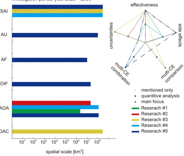
Figure 1-4. The studied CE technologies in this thesis are Sulphate Aerosol Injection (SAI), Artificial Upwelling (AU), Afforestration (AF), Ocean Iron Fertilization (OIF), Artificial Ocean Alkalinization (AOA) and CO² Direct Air Capture (DAC). In the radar diagram to the right side, individual research with related manuscript written as first author, is marked in solid curves (#1, #2, #3, #4), and in dashed curve curve (#5) as second author.

0 0.1 0.2 0.3 0.4 0.5 0.6 0.7 0.8 0.9 1

10⁷ 10⁸ 10⁶

10⁵ 10⁴ 10³ 10² 10¹

spatial scale [km²] SAI

AOA

DAC

effectiveness

side effects

uncertainties

multi-CE comparison multi-CE

combination

main focus

quantitive analysis mentioned only

Reserach #1 Reserach #2 Reserach #3 Reserach #4 investigation period: year 2020 ~ 2099

AF

OIF AU

Reserach #5

(35)

1.5. Publications and Author Contributions

---

Research #1

(E.) Y. Feng (冯玉铭), D. P. Keller, W. Koeve and A. Oschlies (2016): Could artificial ocean alkalinization protect tropical coral ecosystems from ocean acidification?

Environmental Research Letters, 11 (7) [highlighted by journal]

Contributions:

Idea and experimental design: D. P. Keller and Y. Feng Model simulations: Y. Feng

Data analysis: Y. Feng, D. P. Keller, W. Koeve and A. Oschlies

Manuscript preparation: Y. Feng with inputs and comments from D. P. Keller, W.

Koeve and A. Oschlies

---

Research #2

(E.) Y. Feng, W. Koeve, D. P. Keller and A. Oschlies (to be submitted): Model-based assessment of the potential of coastal ocean alkalinization Environmental Research Letters,

Contributions:

Idea and experimental design: Idea is raised by A. Oschlies, W. Koeve and D. P.

Keller, experiment and algorithm designs are undertaken by Y. Feng Modeling simulations: Y. Feng

Data analysis: Y. Feng

(36)

Manuscript preparation: Y. Feng with inputs and comments from W. Koeve, D. P.

Keller and A. Oschlies

---

Research #3

(E.) Y. Feng, D. P. Keller and A. Oschlies (prepared manuscript): Cooling effects from climate feedbacks in climate engineering implementations Journal of Climate (targeted)

Contributions:

Idea and experimental design: Y. Feng and A. Oschlies Modeling simulations: Y. Feng

Manuscript preparation: Y. Feng with inputs and comments from D. P. Keller ---

Research #4

(E.) Y. Feng (prepared manuscript): Modeling assessment of combined SRM/AOA scheme Climatic Change (targeted)

Contributions:

Idea and experimental design: Y. Feng Modeling simulations: Y. Feng

Manuscript preparation: Y. Feng

---

(37)

Research #5

D. P. Keller, (E.) Y. Feng, and A. Oschlies (2014): Potential climate engineering effectiveness and side-effects during a high carbon dioxide emission scenario?

Nature Communications, doi:10.1038 Contributions:

Idea and experimental design: Idea is raised by D. P. Keller, experiment and code designs are undertaken by D. P. Keller and Y. Feng

Modeling simulations: D. P. Keller Data analysis: D. P. Keller

Manuscript preparation: D. P. Keller with comments from A. Oschlies and Y. Feng

(38)

2. Research #1

Could artificial ocean alkalinization protect tropical coral ecosystems from ocean acidification?

Ellias Y. Feng (冯玉铭)^{1, 2}, David P. Keller¹, Wolfgang Koeve¹ and Andreas Oschlies^{1, 2}.

1 GEOMAR Helmholtz Centre for Ocean Research Kiel

2 University of Kiel

1 E-mail: yfeng@geomar.de

Abstract: Artificial ocean alkalinization (AOA) is investigated as a method to mitigate local ocean acidification and protect tropical coral ecosystems during a 21st century high CO2 emission scenario. Employing an Earth system model of intermediate complexity, our implementation of AOA in the Great Barrier Reef, Caribbean Sea and South China Sea regions, shows that alkalinization has the potential to counteract expected 21st century local acidification in regard to both oceanic surface aragonite saturation Ω and surface pCO2. Beyond preventing local acidification, regional AOA, however, results in locally elevated aragonite oversaturation and pCO2 decline. A notable consequence of stopping regional AOA is a rapid shift back to the acidified conditions of the target regions. We conclude that artificial ocean alkalinization may be a method that could help to keep regional coral ecosystems within saturation states and pCO2 values close to present-day values even in a high-emission scenario and thereby might “buy some time” against the ocean acidification threat, even though regional AOA does not significantly mitigate the warming threat.

(39)

2.1. Introduction

Anthropogenic CO² invades the ocean and thereby perturbs ocean chemistry, this phenomenon is also known as “ocean acidification” (e.g. Caldeira and Wickett 2003, Feely et al. 2004). If CO² emissions continue to increase and the ocean continues to become more acidic these changes will further affect the ambient saturation state of aragonite (described by aragonite Ω). Since calcification, which is a crucial skeleton building process for most stony corals, is considered to be highly sensitive to ambient aragonite Ω, coral calcification is likely to become inhibited in the future (Gattuso et al. 1998, Langdon and Atkinson 2005). Stony coral reefs sustain the most diverse ecosystems in the tropical oceans, and the coral-supported tropical fish (Munday et al. 2014), coralline algae (McCoy and Ragazzola 2014), echinoderms (Dupont et al. 2010), molluscs (Gazeau et al. 2007), crustaceans (Whiteley 2011), and corals themselves (Kleypas et al. 1999a, Hoegh-Guldberg et al. 2007, Cao and Caldeira 2008, Crook et al. 2011, Meissner et al. 2012a) are expected to face difficulties in adapting to future ocean conditions in coming decades because of both ocean acidification itself and the loss of the reef structure. A potential loss of coral reefs and their ecosystems may also have a direct impact on coastal resources and services (Brander et al. 2009). Besides the threat from ocean acidification coral reefs face a number of other significant threats such as coral bleaching, which is triggered by persistent heat stress and is thought to be one of the most serious climate change related threats (Hoegh-Guldberg 1999, Cooper et al. 2008, De’ath et al. 2009, Frieler et al. 2012, Caldeira 2013).

(40)

Since efforts to mitigate global warming and ocean acidification by reducing emissions have, up to now, been unsuccessful in terms of a significant reduction in the growth of atmospheric CO² concentrations, there has been growing interest in climate engineering (CE) to mitigate or prevent various consequences of anthropogenic climate change (Crutzen 2006, Schuiling and Krijgsman 2006, Oschlies et al. 2010). For example, several modelling studies have examined “Artificial Ocean Alkalinization (AOA)” which modifies ocean alkalinity. These studies simulated the use of alkalizing agents such as olivine (a Mg-Fe-SiO⁴ mineral) (Köhler et al. 2010, 2013, Hartmann et al. 2013), calcium carbonate (Caldeira and Rau 2000, Harvey 2008), or calcium hydroxide (Ilyina et al. 2013a, Keller et al. 2014) to elevate the ocean’s alkalinity to increase CO² uptake and mitigating ocean acidification. While these simulations suggested that AOA could potentially be used to mitigate global warming and ocean acidification to some degree, some studies also suggested that deploying AOA at a global scale may face prohibitive logistical and economical constraints and could possibly cause undesired side effects (Renforth et al. 2013, Keller et al. 2014).

In this paper we use Earth system model simulations of regional AOA to investigate the potential of AOA to protect specific stony coral reef regions against ocean acidification. We also investigate possible environmental side effects of AOA and possible regional differences in effectiveness or undesired side effects. The model simulations show AOA could mitigate ocean acidification in our investigated coral reef regions, albeit at substantial economic costs and with the termination risk of a rapid return to acidified conditions after the stop of local AOA.

(41)

2.2. Method

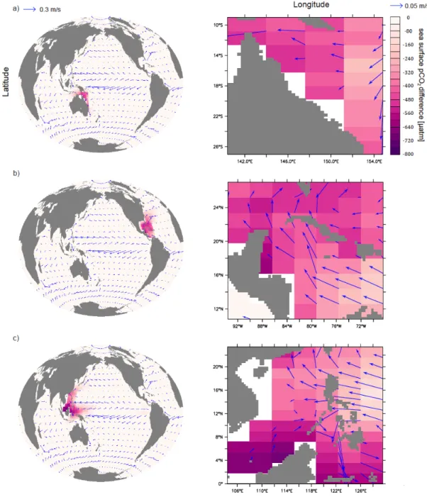
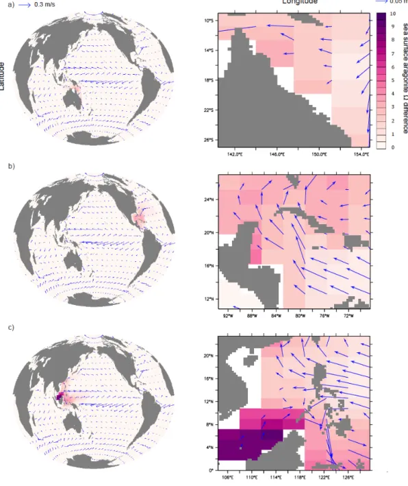
We simulated calcium hydroxide (Ca(OH)2)-based AOA in the Great Barrier Reef (GB, 9.0°S~27.0°S, 140.4°E~154.8°E, an area of 1.7 x 106 km²), the Caribbean Sea (CS, 10.8°N~27°N, 68.4°W~93.6°W, an area of 3.9 x 106 km²) and the South China Sea (SC, 0°N~23.4°N, 104.4°E~129.6°E, an area of 5.2 x 10⁶ km²) (Figure 2-1) using the University of Victoria Earth System Climate Model (UVic) version 2.9. These areas contain some of the world’s most abundant coral reefs (http://www.reefbase.org/) and are large enough to be addressed by the UVic model. From the data obtained from ReefBase (http://www.reefbase.org/), we found that from a total of 10,048 coral reef locations, 3323 are located in the Great Barrier Reef box, 601 in the Caribbean Sea box, and 2060 in the South China Sea box. Altogether 5984 reef points are included in our three regions, which is more than half of the global coral reef locations collected from ReefBase.

The UVic model consists of an energy-moisture balance atmospheric component, a 3D primitive-equation oceanic component that includes a sea-ice sub- component, and a terrestrial component (Weaver et al. 2001, Meissner et al. 2003).

Wind velocities are prescribed from NCAR/NCEP monthly climatological data.

Accordingly, UVic does not feature decadal ocean-atmosphere oscillations, like ENSO. The model has a spatial resolution of 3.6°×1.8° with 19 vertical layers in the ocean. The global carbon cycle is simulated with air-sea gas exchange of CO² and marine inorganic carbonate chemistry following the Ocean Carbon-Cycle Model Intercomparison Project Protocols (Orr et al. 1999). The inorganic carbon cycle is coupled to a marine ecosystem model that includes phytoplankton, zooplankton,

(42)

detritus, the nutrients nitrate and phosphate, and oxygen (Keller et al. 2012). The model has been evaluated in several model intercomparison projects (Eby et al. 2013, Zickfeld et al. 2013, Weaver et al. 2012), and shows a reasonable response to anthropogenic CO² forcing that is well within the range of other models. In order to illustrate that our model is robust in reproducing general ocean circulation and chemistry, we validate our model against GLODAP (Global Ocean Data Analysis Data Project) v1.1 data for ocean total alkalinity and oceanic dissolved inorganic carbon (Key et al. 2004) (Figure A1 and A2 in Appendix A), SOCAT (Surface Ocean CO² Atlas) data (Bakker et al. 2014, Landschützer et al. 2014) for sea surface pCO² (Figure A3), and WOA (World Ocean Atlas) 2013 data for sea surface temperature (Figure A4). The validation illustrates that UVic can generally reproduce the global patterns of surface ocean alkalinity and dissolved inorganic carbon as well as sea surface pCO². UVic’s performance in reconstructing sea surface temperature (SST) is also generally good, especially in regions where AOA is implemented in our study with less than a 0.8 ℃ model-data misfit. Overall, the model-data differences displayed by the UVic model are well within the range data-error bonds from CMIP5 model simulations (Wang et al. 2014, Ilyina et al. 2013b, Jungclaus et al. 2013).

The model was spun-up for 10,000 years under pre-industrial atmospheric and astronomical boundary conditions. From year 1800 to 2005 the model was forced with historical fossil fuel and land-use carbon emissions. Then, from the year 2006 onwards the Representative Carbon Pathway 8.5 (RCP 8.5) anthropogenic CO² emission scenario forcing was used (Meinshausen et al. 2011). CO² is the only greenhouse gas taken into account. Continental ice sheets, volcanic forcing, and

(43)

astronomical boundary conditions were held constant to facilitate the experimental set-up and analysis.

Figure 2-1. Annual-mean surface aragonite Ω and pCO² simulated by the UVic model control run without regional artificial ocean alkalinization (AOA) for preindustrial (a, c) and 2020 (b, d). AOA experimental regions are marked by black boxes. Coral Reef locations are marked in cyan.

Ca(OH)²-based AOA is simulated in an idealized manner by increasing surface alkalinity (Keller et al. 2014). The rationale behind this method is that dissolving one mole of Ca(OH)² in seawater increases total alkalinity by 2 moles (Ilyina et al. 2013a). We simulate Ca(OH)²-based AOA by homogeneously and continuously adding alkalinity to the upper 50m of the targeted regions. In the following, we therefore use the term “lime addition” to refer to our simulated

(44)

current model’s capacity and we therefore focus on AOA-induced impacts on regional and global marine chemistry. Also, we ignore the impact of increasing water temperature on corals, which will accompany elevated levels of atmospheric CO² and would likely also have a detrimental impact on coral reefs.

We use a fixed threshold aragonite Ω to describe suitable stony coral habitats since most of today’s coral reefs are found in waters with ambient seawater aragonite Ω above a critical value (Kleypas et al. 1999b, Meissner et al. 2012a, 2012b, Ricke et al.

2013). However, this approach involves some uncertainties (Kleypas et al. 1999b, Guinotte et al. 2003) due to the neglect of seasonal and diurnal Ω fluctuations, species variety, and species ability to adapt. Critical coral habitat threshold values of ambient aragonite Ω ranging from Ω = 3 (Meissner et al. 2012b), Ω = 3.3 (Meissner et al. 2012a), to Ω = 3.5 (Ricke et al. 2013) have been used in recent climate change studies, acknowledging that these represent regional mean values and that local reef- scale carbonate chemistry may display large diurnal fluctuations also in healthy reefs.

Ignoring sea surface temperature as a regulator of coral reef habitats may be a further simplification (Couce et al. 2013). We follow these earlier studies and, in this paper, use an aragonite Ω threshold of 3 to determine whether or not seawater chemistry with a region is suitable for stony corals.

A healthy coral ecosystem usually includes a multitude of both calcifying and non-calcifying organisms. Aragonite Ω is commonly used to evaluate the impact of ocean acidification on marine calcifying organisms. Nevertheless, ocean acidification can also affect non-calcifying organisms, e.g. by reducing their metabolic rates (Rosa and Seibel 2008) or damaging their larval and juvenile stages (Frommel et al. 2011).

(45)

Concerning non-calcifying organisms, often pCO² is employed as a metric to evaluate impacts of ocean acidification. We therefore also consider how seawater pCO² will develop under increasing atmospheric pCO² and continuous AOA.

Without AOA, annual-mean surface seawater pCO² will follow atmospheric pCO² with some small time lag (e.g. Bates 2007). A meta-study of resistance of different marine taxa to elevated pCO² (Wittmann and Pörtner 2013) found that 50% of the species of corals, echinoderms, molluscs, fishes and crustaceans are negatively affected if seawater pCO² reaches high levels (between 632 to 1,003 µatm) with many species, except for crustaceans, also being significantly affected by pCO² levels between 500-650 µatm. Among the studied species, 57 % of echinoderms and 50 % of molluscs were negatively affected by the lowest levels of experimental pCO² manipulations. Since the loss of even one species, such as a keystone species, could potentially be detrimental for reef health, we chose a relatively low threshold of 500 µatm pCO² (as an annual average) to determine whether or not conditions were suitable for maintaining a healthy reef habitat. Moreover, by choosing a lower threshold we can better account for any variability in pCO² that may not be well simulated by our model. However, we must acknowledge that there are considerable uncertainties concerning such a threshold. Furthermore, these thresholds can be modulated by other environmental factors (Manzello 2015) and may not be absolutely applicable in every reef location. To avoid unnecessary complexity, the thresholds for both pCO² and Ω are considered here in terms of regional and annual averages.