1 Supplemental Information:
The role of host promiscuity in the invasion process of a seaweed holobiont
Guido Bonthond1*, Till Bayer1, Stacy A. Krueger-Hadfield2, Nadja Stärck1, Gaoge Wang3, Masahiro Nakaoka4, Sven Künzel5, Florian Weinberger1
1 GEOMAR Helmholtz Centre for Ocean Research Kiel, Düsternbrooker Weg 20, 24105, Kiel, Germany.
2 Department of Biology, University of Alabama at Birmingham, 1300 University Blvd, CH464, Birmingham, AL, 35294, USA
3 College of Marine Life Sciences and Institute of Evolution and Marine Biodiversity, Ocean University of China, 5 Yushan Road, Qingdao 266003, China
4 Akkeshi Marine Station, Field Science Center for Northern Biosphere, Hokkaido University, Aikappu 1, Akkeshi, Hokkaido 088-1113, Japan
5 Max Planck Institute for Evolutionary Biology, Plön, Germany
* Corresponding author: gbonthond@geomar.de
Table of Contents:
Figure S1 Page 2
Figure S2 Page 3
Figure S3 Page 4
Figure S4 Page 5
Table S1 Sample summary Page 6,7 Table S2 Experiment overview Page 8-10
Table S3 Core OTUs Page 11-15
Table S4 Statistical output Page 16-22
2
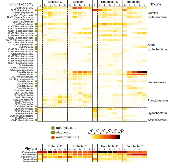
Figure S1. Relative OTU (A) and Phyla (B) abundances displayed in a heatmap by substrate (epi- and
endobiota) and treatment (control and treated). Only the 50 most abundant OTUs and 5 most abundant
Phyla are shown. Columns are ordered in time, starting from left right with the field collection (t
f) and
ending with the final sampling in the experiment (t
6). Rows are ordered by Phylum and abundance. Core
OTUs, identified as geographically independent in Bonthond et al. (2020), are labeled with green
(epiphytic core), red or green-red (geographically conserved in both epi- and endobiota).
3
Figure S2. Changes in community properties between the field and start of the experiment. Panels
display diversity changes in (A: rarefied OTU richness; Sn) and (B: evenness). Predicted functional
groups are displayed in C-F (autotrophy, aerobic heterotrophy, anaerobic heterotrophy and diazotrophy,
respectively)
4
Figure S3. Regression curves of beta-diversity in terms of Bray-Curtis and weighted UniFrac distances.
Diagrams display the mean distance within populations (controls in blue and treated algae in orange; A-
D) and between populations (E-H) over time, between native (black) and non-native (red) controls over
time (I-L) and between native and nonnative treated individuals over time (M-P). The 95% confidence
regions are indicated in shades of the corresponding color. Marginal and conditional R
2values of the
models are displayed in the bottom right corner of the most right panel corresponding to the same
model.
5
Figure S4. Regression curves of Bray-Curtis (A, B) and weighted UniFrac distances (C, D), within
epibiota (A, C) and endobtioa (B, D) with respect to the field. Diagrams display the mean distance with
respect to microbiota in the field for treated native (black) and treated non-native (red) holobionts over
time. The 95% confidence regions are indicated in shades of the corresponding color. Marginal and
conditional R
2values of the models are displayed in the bottom right corner.
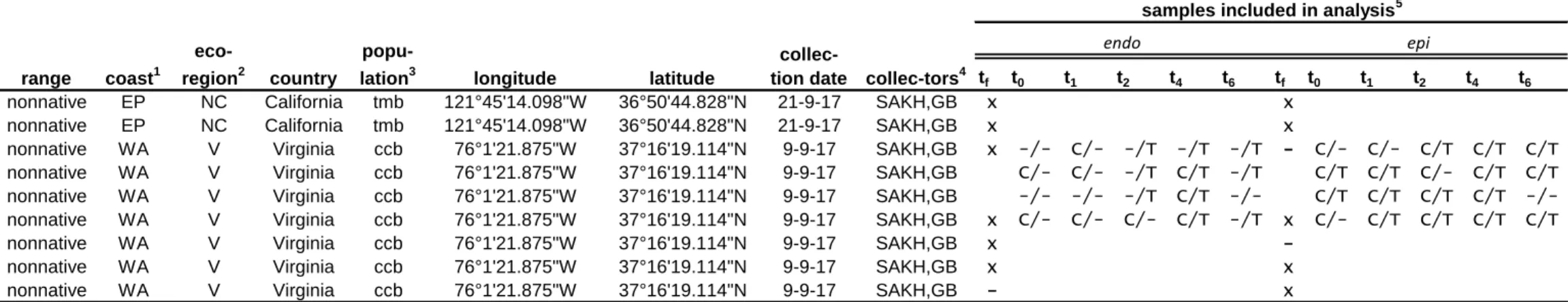
Table S1. Summary of samples remaining after data quality treatment and included in analyses.
tf t0 t1 t2 t4 t6 tf t0 t1 t2 t4 t6 sou1 native WP NH Japan sou 141°3'34.90"E 38°21'10.20"N 27-8-17 MN,FW,TB - -/- C/- C/T -/T -/T x -/T C/T C/T C/T -/T sou2 native WP NH Japan sou 141°3'34.90"E 38°21'10.20"N 27-8-17 MN,FW,TB x -/- -/- -/T -/T -/- x C/T C/T C/T C/T C/- sou5 native WP NH Japan sou 141°3'34.90"E 38°21'10.20"N 27-8-17 MN,FW,TB - C/T C/T -/- C/T C/T x C/T C/T C/T C/T C/T sou6 native WP NH Japan sou 141°3'34.90"E 38°21'10.20"N 27-8-17 MN,FW,TB x -/- -/- C/T -/- -/- x -/T -/T C/T C/T C/-
sou4 native WP NH Japan sou 141°3'34.90"E 38°21'10.20"N 27-8-17 MN,FW,TB - x
sou8 native WP NH Japan sou 141°3'34.90"E 38°21'10.20"N 27-8-17 MN,FW,TB x x
akk4 native WP OC Japan akk 144°56'59.30"E 43°2'51.90"N 31-8-17 MN,TB - C/T C/T C/T -/- -/- x C/T C/T C/- C/T C/T akk7 native WP OC Japan akk 144°56'59.30"E 43°2'51.90"N 31-8-17 MN,TB - C/- -/T C/T C/T -/T x C/T C/T C/- C/T C/T akk8 native WP OC Japan akk 144°56'59.30"E 43°2'51.90"N 31-8-17 MN,TB - C/T C/T C/T C/T -/T x C/T C/T C/- C/T C/T akk9 native WP OC Japan akk 144°56'59.30"E 43°2'51.90"N 31-8-17 MN,TB - C/- -/T C/T C/T -/- x C/T C/T C/- C/T C/T
akk1 native WP OC Japan akk 144°56'59.30"E 43°2'51.90"N 31-8-17 MN,TB - x
akk10 native WP OC Japan akk 144°56'59.30"E 43°2'51.90"N 31-8-17 MN,TB - x
ron3 native WP YS China ron 122°20'44.60"E 37°6'45.70"N 1-9-17 GW,FW x C/T C/- C/- -/T -/- x C/T C/T C/T C/T C/T ron4 native WP YS China ron 122°20'44.60"E 37°6'45.70"N 1-9-17 GW,FW x C/T C/- C/- C/T C/- x C/T C/T C/T C/T C/T ron5 native WP YS China ron 122°20'44.60"E 37°6'45.70"N 1-9-17 GW,FW x C/T C/T C/- C/T C/- x C/T C/T C/T C/T C/T
ron8 native WP YS China ron 122°20'44.60"E 37°6'45.70"N 1-9-17 GW,FW C/- C/T C/- C/T C/T -/T C/T C/T C/T C/-
ron6 native WP YS China ron 122°20'44.60"E 37°6'45.70"N 1-9-17 GW,FW x x
ron9 native WP YS China ron 122°20'44.60"E 37°6'45.70"N 1-9-17 GW,FW x x
fdm4 nonnative EA CS France fdm 1°58'11.30"W 48°30'52.60"N 21-9-17 MV,FW - C/T C/T -/T C/T C/T x -/T C/T -/T C/T C/T
fdm5 nonnative EA CS France fdm 1°58'11.30"W 48°30'52.60"N 21-9-17 MV,FW C/T C/T C/T C/- -/- -/- C/T -/- C/T C/T
fdm6 nonnative EA CS France fdm 1°58'11.30"W 48°30'52.60"N 21-9-17 MV,FW x -/- C/T -/- C/T C/T x -/- C/T -/- C/- C/T fdm9 nonnative EA CS France fdm 1°58'11.30"W 48°30'52.60"N 21-9-17 MV,FW - -/- -/- -/- -/- -/- x -/- C/T -/- -/T C/-
fdm1 nonnative EA CS France fdm 1°58'11.30"W 48°30'52.60"N 21-9-17 MV,FW - x
fdm10 nonnative EA CS France fdm 1°58'11.30"W 48°30'52.60"N 21-9-17 MV,FW x -
nor2 nonnative EA NS Germany nor 8°48'44.65"E 54°29'9.34"N 11-9-17 FW,NS - C/- -/T -/T C/T -/- x C/- C/- C/T C/T C/T nor4 nonnative EA NS Germany nor 8°48'44.65"E 54°29'9.34"N 11-9-17 FW,NS - C/T -/T -/T -/T -/- x C/- C/T C/T C/T C/T nor5 nonnative EA NS Germany nor 8°48'44.65"E 54°29'9.34"N 11-9-17 FW,NS x -/- -/- -/- C/T C/T x -/- C/T C/T C/- C/- nor6 nonnative EA NS Germany nor 8°48'44.65"E 54°29'9.34"N 11-9-17 FW,NS x C/- -/- -/- C/- C/- x C/- C/T C/T -/T C/T
nor1 nonnative EA NS Germany nor 8°48'44.65"E 54°29'9.34"N 11-9-17 FW,NS x x
nor8 nonnative EA NS Germany nor 8°48'44.65"E 54°29'9.34"N 11-9-17 FW,NS - x
tmb84 nonnative EP NC California tmb 121°45'14.098"W 36°50'44.828"N 21-9-17 SAKH,GB x x
tmb72 nonnative EP NC California tmb 121°45'14.098"W 36°50'44.828"N 21-9-17 SAKH,GB C/- C/T C/T C/- C/T C/T C/T C/T C/T C/T tmb73 nonnative EP NC California tmb 121°45'14.098"W 36°50'44.828"N 21-9-17 SAKH,GB C/T C/T C/- C/- -/- C/T C/T -/T C/T C/T tmb85 nonnative EP NC California tmb 121°45'14.098"W 36°50'44.828"N 21-9-17 SAKH,GB C/- C/T C/T -/- C/- C/- C/T -/T C/T C/T tmb75 nonnative EP NC California tmb 121°45'14.098"W 36°50'44.828"N 21-9-17 SAKH,GB x C/T C/T C/T C/- C/T x C/T C/T C/T C/T C/T
tmb17 nonnative EP NC California tmb 121°45'14.098"W 36°50'44.828"N 21-9-17 SAKH,GB x x
endo epi
samples included in analysis5
code collec-tors4
collec- tion date latitude
longitude popu-
lation3 country
eco- region2 coast1
range
Table S1. Continued
tf t0 t1 t2 t4 t6 tf t0 t1 t2 t4 t6
tmb76 nonnative EP NC California tmb 121°45'14.098"W 36°50'44.828"N 21-9-17 SAKH,GB x x
tmb74 nonnative EP NC California tmb 121°45'14.098"W 36°50'44.828"N 21-9-17 SAKH,GB x x
ccb30 nonnative WA V Virginia ccb 76°1'21.875"W 37°16'19.114"N 9-9-17 SAKH,GB x -/- C/- -/T -/T -/T - C/- C/- C/T C/T C/T ccb32 nonnative WA V Virginia ccb 76°1'21.875"W 37°16'19.114"N 9-9-17 SAKH,GB C/- C/- -/T C/T -/T C/T C/T C/- C/T C/T ccb46 nonnative WA V Virginia ccb 76°1'21.875"W 37°16'19.114"N 9-9-17 SAKH,GB -/- -/- -/T C/T -/- C/T C/T C/T C/T -/- ccb50 nonnative WA V Virginia ccb 76°1'21.875"W 37°16'19.114"N 9-9-17 SAKH,GB x C/- C/- C/- C/T -/T x C/- C/T C/T C/T C/T
ccb33 nonnative WA V Virginia ccb 76°1'21.875"W 37°16'19.114"N 9-9-17 SAKH,GB x -
ccb7a nonnative WA V Virginia ccb 76°1'21.875"W 37°16'19.114"N 9-9-17 SAKH,GB x x
ccb3 nonnative WA V Virginia ccb 76°1'21.875"W 37°16'19.114"N 9-9-17 SAKH,GB - x
coast1
eco-
region2 country
samples included in analysis5
endo epi
popu-
lation3 longitude latitude
collec-
tion date collec-tors4
1 Abbreviations for continental coasts: Western Pacific (WP), Eastern Pacific (EP), Western Atlantic (WA) and Eastern Atlantic (EA)
2 Abbreviations for ecoregions: Northeastern Honshu (NH), Oyashio Current (OC), Yeallow Sea (YS), Celtic Seas (CS), North Sea (NS), Northern California (NC) and Virginian (V)
3 Abbreviations for populations: Soukanzan (sou), Akkeshi (akk), Rongcheng (ron), Pleudihen-sur-Rance (fdm), Nordstrand (nor), Tomales Bay (tmb), Cape Charles Beach (ccb)
4 Colllectors are abbreviated by author initials.
5 Crosses indicate field samples with more than 1000 after quality filtering included in the analyses. Samples taken during the experiment and passing the quality filtration steps are displayed as
control/treatment. Dashed indicate samples not passing quality criteria whereas samples not included in the field study or experiment are represented by empty cells code range
day group 1: sou group 2: akk & ron group 3: ccb group: 4 nor group: 5 fdm & tmb date
1 field collection sou (tf) 27-08-2017
2 28-08-2017
3 29-08-2017
4 30-08-2017
5 start acclimation field collection akk (tf) 31-08-2017
6 field collection ron (tf) 01-09-2017
7 02-09-2017
8 03-09-2017
9 04-09-2017
10 05-09-2017
11 start acclimation 06-09-2017
12 water exchange 07-09-2017
13 08-09-2017
14 field collection ccb (tf) 09-09-2017
15 10-09-2017
16 field collection nor (tf) 11-09-2017
17 12-09-2017
18 water exchange start acclimation 13-09-2017
19 water exchange 14-09-2017
20 start acclimation 15-09-2017
21 16-09-2017
22 17-09-2017
23 18-09-2017
24 19-09-2017
25 water exchange water exchange 20-09-2017
26 water exchange field collection fdm & tmb (tf) 21-09-2017
27 water exchange 22-09-2017
28 23-09-2017
29 24-09-2017
30 25-09-2017
31 start acclimation 26-09-2017
32 water exchange water exchange 27-09-2017
33 water exchange 28-09-2017
34 29-09-2017
35 water exchange 30-09-2017
36 01-10-2017
37 start treatment 02-10-2017
38 water exchange 03-10-2017
39 water exchange water exchange 04-10-2017
40 end treatment (t0) 05-10-2017
41 06-10-2017
42 water exchange 07-10-2017
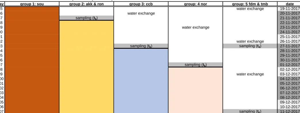
Table S2. Schematic overview of the experiment.
day group 1: sou group 2: akk & ron group 3: ccb group: 4 nor group: 5 fdm & tmb date
43 start treatment 08-10-2017
44 09-10-2017
45 water exchange water exchange 10-10-2017
46 water exchange end treatment (t0) 11-10-2017
47 sampling (t1) 12-10-2017
48 13-10-2017
49 start treatment 14-10-2017
50 15-10-2017
51 16-10-2017
52 water exchange end treatment (t0) start treatment water exchange 17-10-2017
53 water exchange sampling (t1) 18-10-2017
54 sampling (t2) 19-10-2017
55 end treatment (t0) 20-10-2017
56 21-10-2017
57 22-10-2017
58 water exchange water exchange 23-10-2017
59 water exchange sampling (t1) 24-10-2017
60 water exchange sampling (t2) 25-10-2017
61 water exchange 26-10-2017
62 sampling (t1) start treatment 27-10-2017
63 28-10-2017
64 29-10-2017
65 water exchange end treatment (t0) 30-10-2017
66 water exchange sampling (t2) 31-10-2017
67 water exchange 01-11-2017
68 sampling (t4) water exchange 02-11-2017
69 sampling (t2) 03-11-2017
70 04-11-2017
71 water exchange 05-11-2017
72 water exchange sampling (t1) 06-11-2017
73 water exchange 07-11-2017
74 water exchange sampling (t4) 08-11-2017
75 water exchange 09-11-2017
76 10-11-2017
77 11-11-2017
78 water exchange 12-11-2017
79 water exchange sampling (t2) 13-11-2017
80 water exchange sampling (t4) 14-11-2017
81 sampling (t6) 15-11-2017
82 water exchange 16-11-2017
83 sampling (t4) 17-11-2017
84 18-11-2017
Table S2. Schematic overview of the experiment. (continued)
day group 1: sou group 2: akk & ron group 3: ccb group: 4 nor group: 5 fdm & tmb date
85 water exchange 19-11-2017
86 water exchange 20-11-2017
87 sampling (t6) 21-11-2017
88 22-11-2017
89 water exchange 23-11-2017
90 24-11-2017
91 25-11-2017
92 water exchange 26-11-2017
93 sampling (t6) sampling (t4) 27-11-2017
94 28-11-2017
95 29-11-2017
96 30-11-2017
97 sampling (t6) 01-12-2017
98 02-12-2017
99 water exchange 03-12-2017
100 04-12-2017
101 05-12-2017
102 06-12-2017
103 07-12-2017
104 08-12-2017
105 09-12-2017
106 10-12-2017
107 sampling (t6) 11-12-2017
Table S2. Schematic overview of the experiment. (continued)
Group 1 (in red; Soukanzan: sou), group 2 (in yellow; Akkeshi & Rongcheng: akk & ron), group 3 (in blue; Cape Charles Beach: ccb), group 4 (in pink: Nordstrand: nor) and group 5 (Pleudihen-sur-Rance & Tomales Bay: fdm & tmb). The days during which the treated algae were exposed to the antibiotic mix are marked in black. Sampling moments are labelled with tf (in the field) t0, t1, t2, t4 and t6. Right before the application of the treatment and during the rest of the experiment, wet weight was recorded with every water exchange.
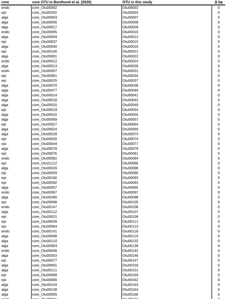
Table S4. Core OTUs identified in this study by cross comparison to Bonthond et al. (2020).
core core OTU in Bonthond et al. (2020) OTU in this study Δ bp
endo core_Otu00002 Otu00002 0
epi core_Otu00202 Otu00003 0
alga core_Otu00003 Otu00007 0
alga core_Otu00006 Otu00008 0
alga core_Otu00017 Otu00009 0
endo core_Otu00005 Otu00010 0
alga core_Otu00004 Otu00014 0
epi core_Otu00037 Otu00015 0
alga core_Otu00040 Otu00019 0
epi core_Otu00146 Otu00021 0
alga core_Otu00001 Otu00022 0
endo core_Otu00012 Otu00024 0
alga core_Otu00013 Otu00026 0
endo core_Otu00007 Otu00031 0
epi core_Otu00061 Otu00035 0
epi core_Otu00025 Otu00037 0
alga core_Otu00070 Otu00038 0
alga core_Otu00477 Otu00040 0
alga core_Otu00014 Otu00041 0
alga core_Otu00018 Otu00043 0
alga core_Otu00015 Otu00049 0
epi core_Otu00019 Otu00054 0
alga core_Otu00010 Otu00055 0
alga core_Otu00069 Otu00057 0
epi core_Otu00027 Otu00064 0
alga core_Otu00024 Otu00069 0
alga core_Otu00028 Otu00073 0
epi core_Otu00030 Otu00074 0
epi core_Otu00044 Otu00077 0
alga core_Otu00078 Otu00079 0
epi core_Otu00076 Otu00081 0
endo core_Otu00082 Otu00084 0
epi core_Otu01112 Otu00086 0
alga core_Otu00016 Otu00088 0
epi core_Otu00059 Otu00090 0
epi core_Otu00166 Otu00093 0
epi core_Otu00592 Otu00094 0
alga core_Otu00057 Otu00095 0
endo core_Otu00067 Otu00097 0
alga core_Otu00390 Otu00098 0
epi core_Otu00098 Otu00105 0
endo core_Otu00147 Otu00106 0
alga core_Otu00112 Otu00107 0
epi core_Otu00021 Otu00109 0
epi core_Otu00039 Otu00111 0
epi core_Otu00064 Otu00113 0
endo core_Otu00141 Otu00118 0
alga core_Otu00008 Otu00119 0
alga core_Otu00110 Otu00132 0
alga core_Otu00063 Otu00138 0
endo core_Otu00048 Otu00142 0
alga core_Otu00303 Otu00146 0
epi core_Otu00077 Otu00147 0
alga core_Otu00091 Otu00150 0
alga core_Otu00111 Otu00151 0
epi core_Otu00068 Otu00160 0
epi core_Otu00080 Otu00162 0
alga core_Otu00104 Otu00163 0
alga core_Otu00148 Otu00164 0
alga core_Otu00055 Otu00166 0
endo core_Otu00041 Otu00174 0
epi core_Otu00058 Otu00177 0
Table S4. Continued
epi core_Otu00065 Otu00178 0
alga core_Otu00286 Otu00180 0
endo core_Otu00086 Otu00184 0
epi core_Otu00949 Otu00187 0
alga core_Otu00109 Otu00195 0
endo core_Otu00236 Otu00199 0
endo core_Otu00193 Otu00203 0
alga core_Otu00150 Otu00204 0
alga core_Otu00383 Otu00206 0
alga core_Otu00066 Otu00212 0
alga core_Otu00174 Otu00219 0
alga core_Otu00574 Otu00224 0
epi core_Otu00103 Otu00241 0
epi core_Otu00960 Otu00246 0
alga core_Otu00169 Otu00247 0
alga core_Otu00128 Otu00248 0
alga core_Otu00134 Otu00256 0
alga core_Otu00154 Otu00257 0
epi core_Otu00087 Otu00258 0
epi core_Otu00094 Otu00262 0
alga core_Otu00182 Otu00272 0
epi core_Otu00546 Otu00281 0
epi core_Otu00270 Otu00286 0
alga core_Otu00323 Otu00290 0
epi core_Otu00649 Otu00293 0
epi core_Otu00235 Otu00295 0
alga core_Otu00413 Otu00301 0
endo core_Otu00140 Otu00312 0
alga core_Otu00149 Otu00316 0
alga core_Otu00516 Otu00321 0
alga core_Otu00137 Otu00322 0
epi core_Otu00356 Otu00325 0
epi core_Otu00221 Otu00326 0
epi core_Otu00168 Otu00328 0
alga core_Otu00117 Otu00332 0
alga core_Otu00219 Otu00333 0
alga core_Otu00187 Otu00335 0
alga core_Otu00675 Otu00343 0
alga core_Otu00304 Otu00354 0
endo core_Otu00339 Otu00359 0
epi core_Otu00184 Otu00363 0
endo core_Otu00319 Otu00377 0
alga core_Otu00225 Otu00381 0
alga core_Otu00344 Otu00388 0
alga core_Otu00172 Otu00389 0
alga core_Otu00549 Otu00408 0
alga core_Otu00294 Otu00419 0
alga core_Otu00460 Otu00421 0
alga core_Otu00326 Otu00433 0
alga core_Otu01267 Otu00435 0
endo core_Otu00347 Otu00437 0
epi core_Otu00259 Otu00439 0
epi core_Otu00643 Otu00452 0
alga core_Otu00283 Otu00460 0
alga core_Otu00454 Otu00477 0
alga core_Otu00277 Otu00495 0
alga core_Otu00288 Otu00496 0
epi core_Otu00586 Otu00504 0
epi core_Otu00375 Otu00527 0
epi core_Otu00512 Otu00539 0
alga core_Otu00204 Otu00561 0
alga core_Otu00622 Otu00578 0
epi core_Otu00686 Otu00580 0
Table S4. Continued
alga core_Otu00991 Otu00586 0
alga core_Otu00291 Otu00598 0
epi core_Otu00228 Otu00606 0
epi core_Otu00439 Otu00625 0
alga core_Otu00485 Otu00634 0
alga core_Otu00285 Otu00635 0
alga core_Otu00536 Otu00655 0
alga core_Otu01057 Otu00658 0
epi core_Otu00382 Otu00659 0
epi core_Otu03335 Otu00674 0
alga core_Otu00994 Otu00697 0
epi core_Otu00295 Otu00709 0
epi core_Otu00320 Otu00730 0
endo core_Otu00783 Otu00733 0
alga core_Otu00504 Otu00740 0
alga core_Otu00669 Otu00776 0
epi core_Otu00412 Otu00799 0
epi core_Otu00522 Otu00801 0
epi core_Otu03089 Otu00807 0
alga core_Otu00814 Otu00811 0
epi core_Otu00640 Otu00814 0
epi core_Otu00275 Otu00825 0
alga core_Otu00691 Otu00833 0
alga core_Otu00445 Otu00838 0
alga core_Otu00613 Otu00875 0
alga core_Otu00380 Otu00920 0
epi core_Otu00679 Otu00923 0
epi core_Otu00537 Otu00941 0
epi core_Otu00583 Otu00979 0
epi core_Otu00612 Otu01000 0
alga core_Otu00937 Otu01010 0
epi core_Otu00774 Otu01019 0
epi core_Otu00690 Otu01038 0
epi core_Otu01126 Otu01047 0
epi core_Otu00557 Otu01094 0
epi core_Otu00972 Otu01141 0
endo core_Otu00970 Otu01151 0
epi core_Otu00695 Otu01158 0
epi core_Otu01312 Otu01166 0
alga core_Otu00563 Otu01173 0
epi core_Otu00391 Otu01174 0
epi core_Otu00654 Otu01178 0
epi core_Otu00476 Otu01217 0
alga core_Otu00573 Otu01250 0
epi core_Otu01553 Otu01254 0
epi core_Otu00876 Otu01255 0
alga core_Otu01398 Otu01266 0
epi core_Otu00466 Otu01269 0
epi core_Otu01006 Otu01328 0
epi core_Otu00934 Otu01355 0
alga core_Otu00580 Otu01362 0
epi core_Otu00651 Otu01369 0
endo core_Otu01181 Otu01387 0
alga core_Otu01208 Otu01490 0
endo core_Otu01365 Otu01527 0
epi core_Otu01292 Otu01606 0
alga core_Otu01128 Otu01607 0
epi core_Otu00595 Otu01653 0
epi core_Otu01150 Otu01738 0
alga core_Otu01331 Otu01839 0
epi core_Otu01119 Otu01878 0
epi core_Otu00384 Otu01884 0
epi core_Otu01249 Otu01987 0
Table S4. Continued
alga core_Otu00195 Otu02072 0
alga core_Otu01634 Otu02096 0
epi core_Otu01076 Otu02127 0
epi core_Otu00562 Otu02147 0
endo core_Otu01796 Otu02165 0
alga core_Otu02433 Otu02311 0
alga core_Otu02051 Otu02314 0
epi core_Otu01325 Otu02323 0
epi core_Otu01728 Otu02400 0
alga core_Otu02469 Otu02408 0
epi core_Otu00936 Otu02436 0
epi core_Otu01474 Otu02450 0
alga core_Otu01261 Otu02473 0
epi core_Otu01529 Otu02571 0
epi core_Otu01772 Otu02613 0
alga core_Otu01218 Otu02882 0
epi core_Otu02486 Otu02895 0
epi core_Otu02197 Otu03205 0
epi core_Otu00740 Otu03274 0
epi core_Otu02052 Otu03354 0
alga core_Otu03263 Otu03618 0
epi core_Otu02087 Otu03646 0
epi core_Otu02863 Otu03828 0
epi core_Otu03011 Otu03893 0
epi core_Otu02067 Otu03916 0
epi core_Otu03326 Otu03920 0
epi core_Otu02759 Otu04080 0
alga core_Otu02610 Otu04452 0
epi core_Otu03076 Otu05089 0
endo core_Otu02787 Otu08149 0
alga core_Otu00020 Otu00016 3
alga core_Otu00023 Otu00029 2
alga core_Otu00034 Otu06204 3
alga core_Otu00035 Otu06508 10
alga core_Otu00052 Otu00123 2
alga core_Otu00083 Otu00709 6
alga core_Otu00089 Otu00251 1
alga core_Otu00130 Otu00044 4
alga core_Otu00133 Otu00126 2
alga core_Otu00153 Otu01039 5
epi core_Otu00155 Otu00709 10
epi core_Otu00179 Otu01189 3
epi core_Otu00197 Otu00059 1
epi core_Otu00199 Otu00727 6
epi core_Otu00200 Otu00340 1
epi core_Otu00216 Otu00912 6
epi core_Otu00218 Otu00337 3
epi core_Otu00230 Otu00273 1
alga core_Otu00242 Otu04147 2
epi core_Otu00245 Otu00413 6
epi core_Otu00262 Otu06481 14
alga core_Otu00269 Otu02079 1
epi core_Otu00280 Otu00760 7
epi core_Otu00290 Otu01757 3
epi core_Otu00298 Otu00624 1
alga core_Otu00300 Otu00577 2
alga core_Otu00301 Otu00534 1
epi core_Otu00322 Otu00837 2
epi core_Otu00332 Otu00900 1
epi core_Otu00343 Otu07111 6
epi core_Otu00370 Otu00405 4
alga core_Otu00387 Otu01104 6
epi core_Otu00406 Otu00670 4
Table S4. Continued
epi core_Otu00416 Otu00125 3
epi core_Otu00421 Otu00230 1
epi core_Otu00422 Otu01193 1
epi core_Otu00441 Otu03376 5
alga core_Otu00446 Otu00259 5
alga core_Otu00461 Otu00369 3
endo core_Otu00468 Otu00445 4
epi core_Otu00470 Otu07593 3
epi core_Otu00568 Otu00271 10
alga core_Otu00633 Otu03661 6
epi core_Otu00652 Otu00509 1
alga core_Otu00658 Otu00884 3
epi core_Otu00684 Otu00693 1
epi core_Otu00731 Otu00633 22
alga core_Otu00749 Otu00278 4
alga core_Otu00755 Otu03833 3
epi core_Otu00766 Otu01660 9
epi core_Otu00784 Otu00246 2
epi core_Otu00791 Otu00831 6
epi core_Otu00902 Otu04165 4
epi core_Otu01105 Otu01592 1
epi core_Otu01289 Otu00909 1
epi core_Otu01299 Otu03245 2
epi core_Otu01412 Otu01200 4
epi core_Otu01426 Otu01929 3
alga core_Otu01454 Otu01702 2
epi core_Otu01514 Otu02302 3
epi core_Otu01539 Otu00091 2
alga core_Otu01544 Otu03231 2
endo core_Otu01585 Otu02358 2
epi core_Otu01594 Otu02246 2
epi core_Otu02159 Otu02808 7
alga core_Otu02183 Otu00580 5
alga core_Otu02188 Otu06067 4
epi core_Otu02221 Otu01310 3
epi core_Otu02388 Otu04680 1
endo core_Otu02399 Otu01298 6
alga core_Otu02654 Otu06117 1
Core types include epi-, endophytic and alga (both epi- and endophytic). OTU numbers and corresponding nucleotide sequences from both studies are shown with the number of nucleotide differences.
Table S3. Statistical output of models fitted in this study. (A) Core abundance
Sum Sq Mean Sq NumDF DenDF F value Pr(>F)
substrate 0.762 0.762 1 115.20 59.763 4.39E-12***
treatment 3.215 1.608 2 114.78 126.018 1.10E-29***
range 0.003 0.003 1 5.12 0.258 0.633
substrate:treatment 0.068 0.034 2 114.51 2.653 0.075 .
substrate:range 0.036 0.036 1 115.20 2.848 0.094 .
treatment:range 0.036 0.018 2 114.78 1.412 0.248
substrate:treatment:range 0.016 0.008 2 114.51 0.629 0.535
Estimate Std. Error df t value Pr(<|t|)
field – treatmentC 0.364 0.026 114.2 13.965 < 2.2E-16***
field – treatmentT 0.308 0.026 115.1 11.904 < 2.2E-16***
treatmentC – treatmentT -0.056 0.030 115.1 -1.895 0.06
.
Table S3. Statistical output of models fitted in this study. (B) Host relative growth rate
Sum Sq Mean Sq NumDF DenDF F value Pr(>F)
range 1665.0 1665.0 1 4.88 7.437 0.043
*
poly(time,3) 9609.3 3203.1 3 364.02 14.307 7.84E-09
***
treatment 439.8 439.8 1 362.86 1.964 0.162
range:poly(time,3) 3312.0 1104.0 3 364.02 4.931 2.28E-03
**
range:treatment 0.0 0.0 1 362.86 0.000 0.998
poly(time,3):treatment 462.7 154.2 3 362.86 0.689 0.559
range:poly(time,3):treatment 147.8 49.3 3 362.86 0.220 0.883
model structure (core/size) ~ substrate * treatment * range + (1|population) + (1|individual)
pairwise comparisons ANOVA table
ANOVA table
model structure ~ range * treatment * poly(time,3) + (1|population) + (1|individual)
Model structures are written in the syntax of the R package lme4 (Bates et al. 2015). The natural logarithm of the sequencing depth is abbreviated with LSD. P-values < 0.05 are displayed in bold and with stars (. < 0.1, * < 0.05, ** < 0.01 and *** < 0.001).
Model structures are written in the syntax of the R package lme4 (Bates et al. 2015). The natural logarithm of the sequencing depth is abbreviated with LSD. P-values < 0.05 are displayed in bold and with stars (. < 0.1, * < 0.05, ** < 0.01 and *** < 0.001).
Table S3. Statistical output of models fitted in this study. (C) α-diversity
Sum Sq Mean Sq NumDF DenDF F value Pr(>F)
timepoint 9300 9300 1 90.687 2.670 0.106
substrate 302685 302685 3 90.586 86.902 6.95E-15***
timepoint:substrate 24499 24499 1 90.835 7.034 9.44E-03**
Estimate Std. Error df t value Pr(>t)
tf:endo – t0:endo -12.664 18.416 90.7 -0.688 0.493
tf:endo – tf:epi -147.589 16.145 90.8 -9.142 1.62E-14***
tf:endo – t0:epi -94.618 18.215 90.9 -5.195 1.25E-06***
t0:endo – tf:epi -134.925 16.602 90.4 -8.127 2.18E-12***
t0:endo – t0:epi -81.954 18.675 90.6 -4.388 3.08E-05***
tf:epi – t0:epi 52.921 16.473 90.8 3.216 1.80E-03**
Sum Sq Mean Sq NumDF DenDF F value Pr(>F)
timepoint 0.886 0.886 1 91.024 1.766 0.187
substrate 33.357 33.357 1 90.878 68.066 1.17E-12***
timepoint:substrate 3.424 3.424 1 91.239 6.988 9.66E-03**
Estimate Std. Error df t value Pr(>t)
tf:endo – t0:endo -0.582 0.218 91.1 -2.666 9.08E-03**
tf:endo – tf:epi -1.591 0.191 91.3 -8.320 8.13E-13***
tf:endo – t0:epi -1.398 0.216 91.3 -6.479 4.60E-09***
t0:endo – tf:epi -1.010 0.197 90.6 -5.129 1.64E-06***
t0:endo – t0:epi -0.816 0.221 90.9 -3.688 3.84E-04***
tf:epi – t0:epi 0.193 0.195 91.1 0.990 0.325
Sum Sq Mean Sq NumDF DenDF F value Pr(>F)
poly(time,3) 161833.771 53944.590 3 356.285 41.230 6.80E-23***
substrate 92291.158 92291.158 1 357.220 70.539 1.08E-15***
treatment 64671.504 64671.504 1 353.675 49.429 1.07E-11***
poly(time,3):substrate 51131.954 17043.985 3 355.817 13.027 4.32E-08***
poly(time,3):treatment 38312.435 12770.812 3 353.698 9.761 3.34E-06***
substrate:treatment 14654.028 14654.028 1 354.586 11.200 9.06E-04***
poly(time,3):substrate:treatment 17259.021 5753.007 3 353.881 4.397 4.70E-03**
Sum Sq Mean Sq NumDF DenDF F value Pr(>F)
poly(time,3) 16.872 5.624 3 358.544 18.032 6.40E-11***
substrate 23.498 23.498 1 359.049 75.339 1.41E-16***
treatment 19.948 19.948 1 355.042 63.959 1.81E-14***
poly(time,3):substrate 3.906 1.302 3 357.992 4.174 6.35E-03**
poly(time,3):treatment 12.832 4.277 3 354.958 13.714 1.75E-08***
substrate:treatment 1.644 1.644 1 356.207 5.271 0.022 *
poly(time,3):substrate:treatment 5.342 1.781 3 355.296 5.709 7.95E-04***
SnSn ANOVA tablePairwise comparisons
logit PIE Pairwise comparisons
model structure
model structure ~ timepoint+ substrate + timepoint:substrate + (1|population) + (1|individual)
ANOVA table
~ poly(time,3)* substrate * treatment + (1|population) + (1|individual)
ANOVA tableANOVA table
Model structures are written in the syntax of the R package lme4 (Bates et al. 2015). Abbreviations are used for natural logarithm of the sequencing depth (LSD), rarefied richness (Sn), probability of interspecific encounter (PIE). P-values < 0.05 are displayed in bold and with stars (. < 0.1, * < 0.05, ** < 0.01 and *** < 0.001).
logit PIE
Table S3. Statistical output of models fitted in this study. (D) Functional groups
Sum Sq Mean Sq NumDF DenDF F value Pr(>F)
LSD 59.053 59.053 1 94.419 246.121 4.80E-28***
timepoint 5.593 5.593 1 90.761 23.310 5.56E-06***
substrate 2.087 2.087 1 89.629 8.697 4.07E-03**
timepoint:substrate 0.488 0.488 1 89.576 2.032 0.157
Sum Sq Mean Sq NumDF DenDF F value Pr(>F)
LSD 65.402 65.402 1 75.177 8180.492 1.81E-78***
timepoint 0.028 0.028 1 94.078 3.474 0.065 .
substrate 0.087 0.087 1 92.059 10.896 1.37E-03**
timepoint:substrate 0.004 0.004 1 91.380 0.451 0.503
Sum Sq Mean Sq NumDF DenDF F value Pr(>F)
LSD 85565.149 85565.149 1 40.512 396.813 1.54E-22***
timepoint 32.049 32.049 1 94.976 0.149 0.701
substrate 525.556 525.556 1 94.730 2.437 0.122
timepoint:substrate 4586.436 4586.436 1 93.556 21.270 1.26E-05***
Sum Sq Mean Sq NumDF DenDF F value Pr(>F)
LSD 32.877 32.877 1 94.199 37.271 2.28E-08***
timepoint 10.794 10.794 1 90.937 12.236 7.27E-04***
substrate 8.430 8.430 1 89.967 9.556 2.65E-03**
timepoint:substrate 8.222 8.222 1 89.926 9.321 2.98E-03**
Sum Sq Mean Sq NumDF DenDF F value Pr(>F)
LSD 183.404 183.404 1 357.512 333.320 4.40E-53***
poly(time,3) 19.401 6.467 3 356.737 11.753 2.33E-07***
substrate 17.100 17.100 1 370.621 31.078 4.78E-08***
treatment 41.819 41.819 1 352.675 76.002 1.13E-16***
poly(time,3):substrate 1.373 0.458 3 355.323 0.832 0.477
poly(time,3):treatment 10.579 3.526 3 354.194 6.409 3.08E-04***
substrate:treatment 2.359 2.359 1 354.257 4.287 0.039 *
poly(time,3):substrate:treatment 4.553 1.518 3 353.217 2.758 0.042 *
Sum Sq Mean Sq NumDF DenDF F value Pr(>F)
LSD 213.861 213.861 1 362.427 16913.021 3.25E-306***
poly(time,3) 0.044 0.015 3 357.883 1.147 0.330
substrate 0.005 0.005 1 373.691 0.389 0.533
treatment 0.015 0.015 1 354.038 1.218 0.270
poly(time,3):substrate 0.329 0.110 3 356.622 8.660 1.46E-05***
poly(time,3):treatment 0.110 0.037 3 355.913 2.892 0.035 *
substrate:treatment 0.109 0.109 1 355.590 8.637 0.004 **
poly(time,3):substrate:treatment 0.089 0.030 3 354.416 2.336 0.073 .
log(aerobic heterotroph) ANOVA table
log(aerobic heterotroph)
sqrt(anaerob ic heterotroph)
log(diazotrop h + 1)log(autotroph) ANOVA table
model structure ~ timepoint + substrate + timepoint:substrate + (1|population) + (1|individual)
ANOVA tableANOVA table
model structure ~ poly(time,3)* substrate * treatment + (1|population) + (1|individual)
ANOVA table
log( autotroph) ANOVA table
Table S3. Statistical output of models fitted in this study. (D) Functional groups (continued)
Sum Sq Mean Sq NumDF DenDF F value Pr(>F)
LSD 103564.419 103564.419 1 348.684 1055.300 1.69E-107***
poly(time,3) 2842.657 947.552 3 358.908 9.655 3.82E-06***
substrate 13.370 13.370 1 372.504 0.136 0.712
treatment 7300.525 7300.525 1 354.734 74.391 2.17E-16***
poly(time,3):substrate 717.194 239.065 3 357.524 2.436 0.065 .
poly(time,3):treatment 2085.315 695.105 3 356.324 7.083 1.23E-04***
substrate:treatment 59.197 59.197 1 356.361 0.603 0.438
poly(time,3):substrate:treatment 608.010 202.670 3 355.281 2.065 0.105
Sum Sq Mean Sq NumDF DenDF F value Pr(>F)
LSD 138.093 138.093 1 270.693 158.212 7.01E-29***
poly(time,3) 38.869 12.956 3 361.681 14.844 3.91E-09***
substrate 0.163 0.163 1 369.715 0.187 0.666
treatment 118.517 118.517 1 356.242 135.783 8.36E-27***
poly(time,3):substrate 6.674 2.225 3 360.147 2.549 0.056 .
poly(time,3):treatment 35.251 11.750 3 357.767 13.462 2.42E-08***
substrate:treatment 3.465 3.465 1 358.171 3.969 0.047 *
poly(time,3):substrate:treatment 1.149 0.383 3 357.309 0.439 0.725
sqrt(anaerobic heterotroph) ANOVA tableANOVA table
log(diazotroph + 1)
Model structures are written in the syntax of the R packages lme4 (Bates et al. 2015). The natural logarithm of the sequencing depth is abbreviated with LSD. P-values < 0.05 are displayed in bold and with stars (. < 0.1, * < 0.05, ** < 0.01 and *** < 0.001).
Table S3. Statistical output of models fitted in this study. (E) mGLMs
mod I
Res.Df Df.diff Dev Pr(>dev)
(Intercept) 268 NA NA NA
LSD 267 1 25409.99 0.002
**
population 261 6 77355.52 0.002
**
mod II
Res.Df Df.diff val(F) Pr(>F)
(Intercept) 268 NA NA NA
poly(time,3) 265 3 10751.069 0.004
**
treatment 263 2 4472.002 0.004
**
poly(time,3):treatment 260 6 858.745 0.004
**
mod I
Res.Df Df.diff Dev Pr(>dev)
(Intercept) 182 NA NA NA
LSD 181 1 16491.06 0.002
**
population 175 6 40095.79 0.006
**
mod II
Res.Df Df.diff val(F) Pr(>F)
(Intercept) 182 NA NA NA
poly(time,3) 179 3 3285.973 0.004
**
treatment 177 2 2365.377 0.004
**
poly(time,3):treatment 174 6 642.136 0.004
**
Model structures are written in the syntax of the R package mvabund (Wang et al. 2012). The natural logarithm of the sequencing depth is abbreviated with LSD. p-values < 0.05 are displayed in bold and with stars (. < 0.1, * < 0.05, ** < 0.01 and *** < 0.001).
endobiota
community matrix ~ LSD + pop
ANOVA table
residuals model I ~ poy(time,3) * treatment
ANOVA table
epibiota
community matrix ~ LSD + pop
ANOVA table
residuals model I ~ poly(time,3) * treatment
ANOVA table
Table S3. Statistical output of models fitted in this study. (F) β-diversity
Sum Sq Mean Sq NumDF DenDF F value Pr(>F)
poly(time, 3) 0.351 0.117 3 1136.138 143.430 8.25E-79***
treatment 0.324 0.324 1 1113.915 396.503 1.03E-75***
range 0.015 0.015 1 13.051 17.880 9.78E-04***
pop 0.019 0.019 1 13.165 23.685 2.97E-04***
poly(time, 3):treatment 0.169 0.056 3 1133.769 69.187 4.34E-41***
poly(time, 3):range 0.110 0.037 3 1142.264 45.025 1.67E-27***
poly(time, 3):pop 0.051 0.017 3 1127.385 20.911 3.46E-13***
treatment:range 0.015 0.015 1 1118.174 18.787 1.59E-05***
treatment:pop 0.013 0.013 1 1108.682 16.525 5.14E-05***
poly(time, 3):treatment:range 0.062 0.021 3 1138.261 25.136 9.50E-16***
poly(time, 3):treatment:pop 0.013 0.004 3 1127.107 5.223 0.001**
Sum Sq Mean Sq NumDF DenDF F value Pr(>F)
poly(time, 3) 0.069 0.023 3 504.683 17.770 5.59E-11***
treatment 0.012 0.012 1 485.917 9.160 0.003**
range 0.013 0.013 1 12.957 10.387 0.007**
pop 0.012 0.012 1 13.470 9.443 0.009**
poly(time, 3):treatment 0.034 0.011 3 489.090 8.854 1.00E-05***
poly(time, 3):range 0.076 0.025 3 513.655 19.624 4.66E-12***
poly(time, 3):pop 0.009 0.003 3 512.790 2.218 0.085 .
treatment:range 0.044 0.044 1 493.691 33.842 1.08E-08***
treatment:pop 0.000 0.000 1 487.338 0.019 0.891
poly(time, 3):treatment:range 0.008 0.003 3 493.261 1.987 0.115
poly(time, 3):treatment:pop 0.002 0.001 3 487.688 0.556 0.645
Sum Sq Mean Sq NumDF DenDF F value Pr(>F)
poly(time, 3) 0.041 0.014 3 1151.684 68.894 5.59E-41***
treatment 0.009 0.009 1 1119.572 46.017 1.89E-11***
range 0.005 0.005 1 12.110 26.239 2.45E-04***
pop 0.004 0.004 1 12.639 19.273 7.80E-04***
poly(time, 3):treatment 0.012 0.004 3 1145.278 20.677 4.74E-13***
poly(time, 3):range 0.010 0.003 3 1158.093 16.583 1.49E-10***
poly(time, 3):pop 0.002 0.001 3 1139.416 2.717 0.043*
treatment:range 0.004 0.004 1 1123.783 21.144 4.74E-06***
treatment:pop 0.000 0.000 1 1111.731 1.825 0.177
poly(time, 3):treatment:range 0.003 0.001 3 1149.717 4.578 0.003**
poly(time, 3):treatment:pop 0.000 0.000 3 1136.229 0.732 0.533
Sum Sq Mean Sq NumDF DenDF F value Pr(>F)
poly(time, 3) 0.004 0.001 3 502.287 8.274 2.21E-05***
treatment 0.000 0.000 1 485.397 0.434 0.510
range 0.001 0.001 1 12.492 6.504 0.025*
pop 0.001 0.001 1 13.367 4.533 0.052 .
poly(time, 3):treatment 0.003 0.001 3 487.402 4.896 0.002**
poly(time, 3):range 0.007 0.002 3 510.938 12.943 3.68E-08***
poly(time, 3):pop 0.001 0.000 3 509.883 2.080 0.102
treatment:range 0.000 0.000 1 493.047 1.144 0.285
treatment:pop 0.000 0.000 1 486.540 0.329 0.567
poly(time, 3):treatment:range 0.002 0.001 3 490.971 3.099 0.027*
poly(time, 3):treatment:pop 0.000 0.000 3 486.451 0.835 0.475
epi - Bray-Curtis distances
model structure
epi - UniFrac distances ANOVA table
endo - UniFrac distances ANOVA table
endo - Bray-Curtis distances
~ poly(time,3) * treatment * (range + pop) + (1|population) + (1|individual)
Model structures are written in the syntax of the R packages lme4 (Bates et al. 2015). The natural logarithm of the sequencing depth is abbreviated with LSD. P-values < 0.05 are displayed in bold and with stars (. < 0.1, * < 0.05, ** < 0.01 and *** < 0.001).
ANOVA tableANOVA table
Table S3. Statistical output of models fitted in this study. (G) Relative to field
Sum Sq Mean Sq NumDF DenDF F value Pr(>F)
poly(time, 3) 0.047 0.016 3 464.259 20.233 2.44E-12***
range 0.009 0.009 1 115.694 11.234 0.001 **
poly(time, 3):range 0.041 0.014 3 464.259 17.820 5.80E-11***
Sum Sq Mean Sq NumDF DenDF F value Pr(>F)
poly(time, 3) 0.008 0.003 3 169.762 3.860 0.011 *
range 0.000 0.000 1 77.735 0.341 0.561
poly(time, 3):range 0.006 0.002 3 169.762 2.658 0.050 *
Sum Sq Mean Sq NumDF DenDF F value Pr(>F)
poly(time, 3) 0.007 0.002 3 470.157 9.711 3.15E-06***
range 0.006 0.006 1 116.181 27.309 7.73E-07***
poly(time, 3):range 0.014 0.005 3 470.157 20.035 3.10E-12***
Sum Sq Mean Sq NumDF DenDF F value Pr(>F)
poly(time, 3) 0.003 0.001 3 160.786 15.302 8.33E-09***
range 0.000 0.000 1 77.233 2.595 0.111
poly(time, 3):range 0.000 0.000 3 160.786 1.122 0.342
epi - Bray- Curtisendo - Bray- Curtisepi - UniFrac ANOVA table
endo - UniFrac ANOVA table
Model structures are written in the syntax of the R packages lme4 (Bates et al. 2015). The natural logarithm of the sequencing depth is abbreviated with LSD. P-values < 0.05 are displayed in bold and with stars (. < 0.1, * < 0.05, ** < 0.01 and *** < 0.001).
ANOVA table
model structure ~ poly(time,3) * individual * range + (1|individual)
ANOVA table