The 2018 northern European hydrological drought and its drivers in a historical perspective

(1)

Hydrol. Earth Syst. Sci., 24, 5621–5653, 2020 https://doi.org/10.5194/hess-24-5621-2020

The 2018 northern European hydrological drought and its drivers in a historical perspective

Sigrid J. Bakke¹, Monica Ionita², and Lena M. Tallaksen¹

1Department of Geosciences, University of Oslo, Oslo, Norway

2Alfred Wegener Institute, Helmholtz Centre for Polar and Marine Research, Bremerhaven, Germany Correspondence:Sigrid J. Bakke (s.j.bakke@geo.uio.no)

Received: 19 May 2020 – Discussion started: 18 June 2020

Revised: 25 September 2020 – Accepted: 1 October 2020 – Published: 26 November 2020

Abstract. In 2018, large parts of northern Europe were affected by an extreme drought. A better understanding of the characteristics and the large-scale atmospheric circulation driving such events is of high importance to enhance drought forecasting and mitigation. This paper examines the historical extremeness of the May–August 2018 meteorological situation and the accompanying meteorological and hydrological (streamflow and groundwater) drought. Further, it investi- gates the relation between the large-scale atmospheric circulation and summer streamflow in the Nordic region. In May and July 2018, record-breaking temperatures were observed in large parts of northern Europe associated with blocking systems centred over Fennoscandia and sea surface temperature anomalies of more than 3^◦C in the Baltic Sea. Extreme meteorological drought, as indicated by the 3-month Stan- dardized Precipitation Index (SPI3) and Standardized Pre- cipitation Evapotranspiration Index (SPEI3), was observed in May and covered large parts of northern Europe by July.

Streamflow drought in the Nordic region started to develop in June, and in July 68 % of the stations had record-low or near- record-low streamflow. Extreme streamflow conditions persisted in the southeastern part of the region throughout 2018.

Many groundwater wells had record-low or near-record-low levels in July and August. However, extremeness in groundwater levels and (to a lesser degree) streamflow showed a diverse spatial pattern. This points to the role of local terrestrial processes in controlling the hydrological response to meteorological conditions. Composite analysis of low summer streamflow and 500 mbar geopotential height anomalies revealed two distinct patterns of summer streamflow variability: one in western and northern Norway and one in the rest of the region. Low summer streamflow in western and

northern Norway was related to high-pressure systems centred over the Norwegian Sea. In the rest of the Nordic region, low summer streamflow was associated with a high-pressure system over the North Sea and a low-pressure system over Greenland and Russia, resembling the pattern of 2018. This study provides new insight into hydrometeorological aspects of the 2018 northern European drought and identifies large- scale atmospheric circulation patterns associated with summer streamflow drought in the Nordic region.

1 Introduction

From May and throughout the summer of 2018, the northern and parts of central Europe experienced drought and record- breaking and persistent high temperatures, leading to severe impacts across a range of sectors (Table 1). Drought is a complex phenomenon characterised by below average natural water availability affecting all components of the hydrological cycle. Unlike most other natural hazards, it is a “creeping phenomenon” with a wide range of economic, societal, and environmental impacts gradually accumulating over time and space (Stahl et al., 2016; Mishra and Singh, 2010; Tallaksen and Van Lanen, 2004).

In 2018, wild fires destroyed vast areas in northern and central Europe. Sweden was especially impacted, with a record-breaking 24 310 ha (835 % of annual average) of burnt area (Table 1a). The drought also led to a significant drop in EU cereal production, whereas beef production grew more than expected due to increased slaughter following fodder shortage (Table 1b). In Scandinavia and Germany, wheat and barley yields were described as catastrophically low (Ta-

(2)

5622 S. J. Bakke et al.: The 2018 northern European hydrological drought and its drivers

Table 1.Reports and news articles about 2018 heat- and drought-related impacts. The impact categories follow the European Drought Impact Report Inventory (EDII; Stahl et al., 2016).

Ref. Impact category Region Publisher URL

(last updated/last accessed)

(a) Wildfires Europe Joint Research Centre,

European Commission

https://op.europa.eu/en/publication-detail/- /publication/435ef008-14db-11ea-8c1f- 01aa75ed71a1/language-en

(29 November 2018/24 March 2020) (b) Agriculture and

livestock farming

European Union Agriculture and Rural Development, European Commission

https://ec.europa.eu/info/news/drop-eu-cereal- harvest-due-summer-drought-2018-oct-03_en (31 October 2019/24 March 2020)

(c) Agriculture and livestock farming

European Union Reuters https://www.reuters.com/article/us-europe-grains- analyst/analysts-cut-eu-wheat-crop-outlook- again-on-catastrophic-north-idUSKBN1KU15E (9 August 2018/24 March 2020)

(d) Agriculture and livestock farming (mainly)

Europe Euronews https://www.euronews.com/2018/08/10/explained- europe-s-devastating-drought-and-the-countries- worst-hit

(12 August 2018/24 March 2020) (e) Agriculture and

livestock farming

Sweden Swedish Board of

Agriculture

https://www2.jordbruksverket.se/download/

18.21625ee16a16bf0cc0eed70/1555396324560/

ra19_13.pdf (16 April 2019/24 March 2020) (f) Agriculture and

livestock farming

Norway Norwegian Agriculture

Agency

https://www.landbruksdirektoratet.no/no/statistikk/

landbrukserstatning/klimarelaterte-skader-og- tap/avlingssvikt-statistikk

(2 September 2019/24 March 2020) (g) Energy and

industry

Norway, Sweden, Finland

Norwegian Water Resources and Energy Directorate

https://www.nve.no/Media/7385/q3_2018.pdf (17 October 2018/24 March 2020)

(h) Energy and industry

Norway newsinenglish.no https://www.newsinenglish.no/2018/07/13/drought- blamed-for-high-electricity-rates/

(13 July 2018/24 March 2020) (i) Waterborne

transportation

Germany Handelsblatt Today https://www.handelsblatt.com/english/companies/low- water-dwindling-rhine-paralyzes-shipping-

transport/23695020.html

(27 November 2018/24 March 2020) (j) Waterborne

transportation

Hungary Reuters https://www.reuters.com/article/us-europe- weather-hungary-shipping/water-levels-in-danube- recede-to-record-lows-hindering-shipping-in- hungary-idUSKCN1L71DH

(22 August 2018/24 March 2020)

(3)

S. J. Bakke et al.: The 2018 northern European hydrological drought and its drivers 5623 Table 1.Continued.

Ref. Impact category Region Publisher URL

(last updated/last accessed)

(k) − Germany Deutsche Welle https://www.dw.com/en/hot-weather-exposes-

world-war-ii-munitions-in-german-waters/a- 44924959 (2 August 2018/24 March 2020) (l) − Czech Republic Business Insider https://www.businessinsider.com/sinister-hunger-

stones-dire-warnings-surfaced-europe-2018- 8?r=US&IR=T (27 August 2018/24 March 2020) (m) Freshwater

ecosystems

Norway Adresseavisen https://www.adressa.no/nyheter/trondelag/2018/07/28/

Gaula-stengt-for-fiske-på-grunn-av-varmen- 17208221.ece

(30 July 2018/24 March 2020)

(n) Public water supply Sweden The Local Sweden https://www.thelocal.se/20190425/sweden- may-be-heading-for-a-new-water-crisis (25 April 2019/24 March 2020)

ble 1c–f). Ecosystems in northern Europe are less adapted to extremely dry conditions as compared to other European regions, and direct negative impacts on terrestrial ecosys- tem productivity were both significantly higher and more widespread in 2018 compared to the more southerly located extreme drought in 2003 (Buras et al., 2020). Already in June, the water volumes in Nordic hydropower reservoirs dropped well below normal, which together with high fuel prices caused the July–August power rates to be the highest in 20 years (Table 1g, h). Record low river levels disrupted main inland waterways in central Europe, forcing transportation ships to reduce their loads by up to 85 % (Table 1i, j).

Low water levels in the river Elbe exposed World War 2 munitions (Table 1k) and so-called hunger stones with centuries- old low water level marks along with dire warnings (Ta- ble 1l). Extremely low streamflow and high river temperatures led to fishing bans in major salmon fishing rivers in Norway (Table 1m). Low groundwater tables led Swedish municipalities to ban residents from using water from the municipal network for anything other than drinking (Ta- ble 1n). The high costs and wide range of impacts associated with the 2018 drought emphasise the need to improve the understanding of such extreme high-impact events affecting large regions in Europe. The latter requires transnational data and international collaboration for in-depth analyses.

To understand how the severity and timing of impacts vary among and within drought-affected areas, it is important to distinguish between different stages of drought development.

Typically, three types of drought are distinguished, reflecting the propagation of drought through the hydrological cycle:

meteorological, soil moisture, and hydrological (streamflow and groundwater) drought (Tallaksen and Van Lanen, 2004).

Meteorological drought refers to a precipitation deficit often combined with abnormally high (potential) evapotranspiration. If a meteorological drought is sustained, it typically

causes soil moisture drought, which mainly concerns water deficits in the root zone impacting water uptake by vegetation (Van Loon, 2015). When soil moisture depletes, a positive feedback loop may occur due to a reduction in the la- tent heat flux (less energy is used for evapotranspiration) and an associated increase in the sensible heat flux (more energy is used to heat the air), which in turn increases the near- surface temperature (Seneviratne et al., 2010). Soil moisture drought can further reduce groundwater recharge and water sources that feed streams and rivers. This may, depending on the catchment characteristics and initial hydrological conditions, lead to groundwater and streamflow drought (Tallak- sen and Van Lanen, 2004). Several studies have demonstrated how meteorological and hydrological droughts develop dif- ferently in space and time (e.g. Barker et al., 2016; Kumar et al., 2016; Haslinger et al., 2014; Vidal et al., 2010; Tallak- sen et al., 2009; Peters et al., 2003; Changnon, 1987). The delay between a meteorological and a hydrological drought may amount to several months, with groundwater typically being the last to react and the last to recover (Hisdal and Tal- laksen, 2000). The conceptdrought, unless specified, refers broadly to the multifaceted phenomenon that includes all three types of drought, along with their specific characteristics.

Many large-scale studies on drought focus on the meteorological aspect, such as anomalies in precipitation or climatic water balance (i.e. precipitation minus potential evapotranspiration), as this is based on data often easily at hand (e.g.

Ionita et al., 2017; Stagge et al., 2017; Vicente-Serrano et al., 2014; Bordi et al., 2009). As opposed to meteorological data, transboundary near-real-time observations of hydrological variables are generally lacking, making timely observation- based large-scale soil moisture, streamflow, or groundwater drought assessments challenging (Liu et al., 2018; Laaha et al., 2016; Hannah et al., 2011). Long-term observational

(4)

5624 S. J. Bakke et al.: The 2018 northern European hydrological drought and its drivers soil moisture data are sparse except for satellite-based esti-

mates covering only a few centimetres depth (Hirschi et al., 2014; Kerr, 2007), which is too shallow to include the root zones of main vegetation types (e.g. Yang et al., 2016;

Schenk and Jackson, 2002). Updated streamflow and groundwater level observations usually need to be collected in a country-by-country manner, which is time consuming as well as challenging due to differences in agency structure, data quality requirements, availability of physiographic proper- ties, and information on human influence. Despite these chal- lenges, research on large-scale droughts cannot rely solely on meteorological data (Van Lanen et al., 2016). Drought assessments using hydrological data are needed to investigate the drought footprint on water resources, which is of high importance for hydropower, navigation, water use sectors, and freshwater ecosystems among others (Laaha et al., 2016; Stahl et al., 2016).

A key natural driver of drought is persistent high-pressure systems leading to prolonged periods of low precipitation and/or high evapotranspiration (Tallaksen and Van Lanen, 2004). To improve drought forecasts and projections, we therefore need a better understanding of the relation between the different types of drought and their large-scale atmospheric and oceanographic drivers. Stationary Rossby waves have been found to play an important role in the development of summer patterns of monthly surface temperature and precipitation variability across northern Eurasia, and they ap- pear to have led to the extreme heat wave and drought in 2003 and 2010 (Schubert et al., 2014, 2011). Kingston et al.

(2015) found that the most widespread and long-duration meteorological droughts in Europe fall into two categories:

northern European droughts with onsets associated with an Atlantic meridional-dipole atmospheric circulation anomaly similar to the North Atlantic Oscillation (NAO) and droughts elsewhere in Europe associated with anomalies related to a northeastward expansion of the Azores High, resembling an eastern Atlantic/western Russia (EA/WR) atmospheric circulation pattern. Fleig et al. (2011) investigated the relation between various circulation types and streamflow drought in Denmark and Great Britain. They found that hydrological droughts are most frequently linked to circulation types representing a high-pressure system over the region affected by drought, which promote hydrological drought development by advection of warm dry air. In addition to stationary high- and low-pressure systems, sea surface temperatures associated with large-scale climate modes of variability have also been found to be important drivers for dryness and wetness variability over Europe (Ionita et al., 2015, 2012). In a study of streamflow drought in Great Britain, Kingston et al. (2013) found statistically significant sea surface temperature and atmospheric anomalies linked to drought onset. The authors emphasise the shortcomings in the ability of circulation indices (such as NAO) to capture fully the atmospheric varia- tion preceding drought onsets, highlighting the value of com-

posite analysis in developing an improved understanding of ocean–atmosphere–drought connections.

The 2018 event was unique in the northern location of the high-pressure system initiating the drought, as compared to other major European drought events in the last decades (Ionita et al., 2017; Stahl, 2001). The affected Nordic region (Norway, Denmark, Sweden, and Finland) exhibits a high heterogeneity in terrestrial and hydroclimatological characteristics. Despite its rather limited size, the region spans several latitudes and has a pronounced west–east gradient in climate and topography, ranging from high mountains in the west to low-lying regions in the south and east. Prevailing westerly winds run northeastwards from the Atlantic, bringing abundant rainfall along the west coast. Orographic effects lead to large local variability in precipitation in the western part of the region. Denmark, southern Sweden, and the western coast of Norway have a maritime climate, in con- trast to the more continental climate in eastern Norway, Swe- den, and Finland. The landscape is largely affected by the last glaciations, with typical landforms such as U-shaped valleys, fjords, and lakes, as well as a large spatial heterogeneity in glacial deposits. Land cover varies with vast areas of bare rock and shallow deposits in the west and north; undulating inland areas characterised by numerous lakes, forests, and wetlands; and areas in the south with thick soils and large aquifers (e.g. Sømme, 1960). Combined with the important effect of seasonal snow on hydrology, varying with latitude and altitude, excluding the very south, the result is a high diversity in hydroclimatological conditions.

In depth analyses of historical drought events, what trig- gers them, and how they manifest themselves in the hydrological cycle enable us to increase our understanding of this complex phenomenon, which is vital to enhance drought forecasting, projection, and mitigation. Motivated by these considerations, this paper focuses on characterising the 2018 drought in northern Europe in a historical context. Tradi- tionally, anomaly maps (in absolute or relative terms) have been used to characterise the meteorological situation of past European events and their spatio-temporal development. Re- cent examples include events such as the major European droughts in 2003 (Black et al., 2004), 2010 (Barriopedro et al., 2011), and 2015 (Ionita et al., 2017). Ranking maps are another way of communicating the extremeness of an event in a long-term perspective, which is simple and easy to com- municate (e.g. Ionita et al., 2017). By ranking the events selected from a time series (e.g. one value each year) according to their magnitude (e.g. temperature), one can map the rank of a particular event, compared to all other years on record, across a region of interest. In this study, we embed both of these approaches, i.e. mapping 2018 anomalies relative to a period of reference (1971–2000) and ranking maps for the 2018 event based on the 60-year period 1959–2018.

The aim of the study is twofold: (1) to investigate the extremeness of the 2018 situation and the accompanying meteorological and hydrological drought in northern Europe and

(5)

S. J. Bakke et al.: The 2018 northern European hydrological drought and its drivers 5625 (2) to identify large-scale atmospheric circulations associated

with below-normal summer streamflow in the Nordic region.

The latter is investigated using empirical orthogonal func- tions (EOFs), which is a well-known method to detect spatial patterns of variability and how they change with time. In Ionita et al. (2015), EOFs are used to study the variability in meteorological drought in Europe and its relation to geopotential height, which is similar to the approach adopted here for the main patterns of summer streamflow variability.

The paper is organised as follows: the data and methods are described in Sects. 2 and 3, respectively. In Sect. 4 (Results), the 2018 meteorological situation (Sect. 4.1), meteorological drought (Sect. 4.2), and hydrological drought (Sect. 4.3) are presented, and the relation between summer streamflow and large-scale atmospheric circulation is investigated (Sect. 4.4). A detailed discussion is provided in Sect. 5, followed by the conclusion in Sect. 6.

2 Data

2.1 Meteorological data

Meteorological data used in this study comprise the 500 mbar geopotential height (HGT500), the zonal and meridional wind, sea surface temperature (SST), air temperature, and precipitation. Monthly data of HGT500 and zonal and meridional wind, used to describe the atmospheric circulation, were extracted from the NCEP-NCAR (National Centers for Atmospheric Prediction and the National Center for Atmo- spheric Research) 40-year reanalysis project (Kalnay et al., 1996). These datasets are available from 1948 to the near- present and have a global coverage on a 2.5^◦ spatial resolution grid. SST data were extracted from the Hadley Cen- tre Sea Ice and Sea Surface Temperature dataset (HadISST;

Rayner et al., 2003), consisting of monthly SST from Jan- uary 1805 to the near-present on a global scale with a spatial resolution of 1^◦spatial resolution.

Europe-wide (35.5–71.5^◦N and 11.0^◦W–42.0^◦E) daily total precipitation and daily maximum, minimum, and mean air temperatures on a 0.1^◦spatial grid were derived from the E-OBS dataset version 21.0e (Cornes et al., 2018). The E- OBS dataset is based on the European Climate Assessment and Dataset station information (ECA&D) and consists of daily data from 1 January 1950 until the near-present.

2.2 Hydrological data

Hydrological data used include time series of streamflow and groundwater levels from stations in the Nordic region.

Streamflow measured at a given point reflects the accumulated responses to precipitation over space and time, whereas groundwater levels represent the lagged response in groundwater over an area varying with local conditions. Streamflow data stem from gauges in Norway, Sweden, Denmark, and Finland. Quality-controlled daily observational streamflow

time series were provided by the Norwegian Water Resources and Energy Directorate (NVE), the Danish Environment Por- tal for Denmark, the Swedish Meteorological and Hydrologi- cal Institute (SMHI), and the Finnish Environmental Institute (SYKE). All gauges had near-natural catchments, i.e. limited or no human interventions (such as reservoirs or water abstractions) influencing the streamflow. Only gauges having less than 10 d with missing values between May and September each year in the 60-year period January 1959–

December 2018 were chosen.

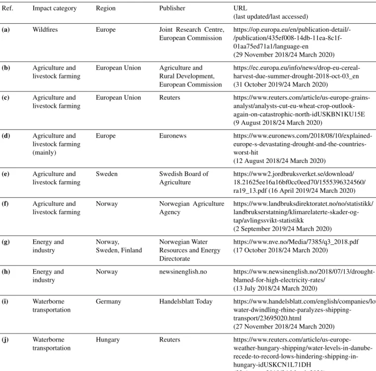
The resulting dataset consisted of time series from 79 gauges, with catchment areas ranging from 6.6 to 10 864 km² (median of 276 km²). Figure 1 shows the locations of the gauges as well as the streamflow regime at each site, reflecting the typical streamflow variability over the year. The regime classification is based on Gottschalk et al. (1979) and calculated for the period 1959–2018 (a detailed description of the classification procedure is provided in Appendix A1).

The five regimes are classified according to whether the streamflow is dominated by (1) winter high flow and summer low flow, mainly due to high evapotranspiration during summer (Atlantic regime); (2) winter low flow and spring high flow, due to snow accumulation and snowmelt (Moun- tain regime); or (3)–(5) various combinations of these two patterns (Baltic, Transition, and Inland regimes). Three of the stations with a Mountain regime (marked with crosses) experience high flows during late summer due to a high percentage (>30 %) of glaciers in their catchments. Standard- ised monthly streamflow statistics for each station are shown in Figs. S3–S5 in the Supplement.

Observed time series of near-natural groundwater levels, i.e. data from stations with limited or no human influence (such as water abstractions), are even less accessible than streamflow data. This includes the necessary metadata with local site information. As a result, the groundwater analysis was limited to data from stations in Norway and Swe- den, provided by NVE and the Geological Survey of Sweden (SGU), respectively. The time series were quality controlled at the host institutions; however, a visual inspection was per- formed to delete potential erroneous outliers. Groundwater level time series were generally shorter than the streamflow time series, and rather than a 60-year period as used for streamflow, a 30-year period (1989–2018) was selected as a balance between the number of stations and the record length.

In a majority of the groundwater wells, observations were taken on a weekly to monthly basis in most of the period.

In Norway, daily or sub-daily measurements were available from the beginning of the 21st century. Half of the Swedish wells had daily or sub-daily measurements from 2016 onwards, whereas the other half had a coarser temporal resolution across the whole 30-year period. Only groundwater stations with at least one monthly measurement during April–

September over the 30-year period analysed were selected.

Groundwater has in many cases a slow response and thus

(6)

Figure 1.Locations and streamflow regimes (based on Gottschalk et al., 1979) of the 79 streamflow stations used in the study. The right panels show plots of mean monthly standardised (i.e. subtracted the mean and divided by the standard deviation) streamflow for each regime (indicated by thin lines) together with the regime mean streamflow (bold line).

holds valuable information at a monthly resolution (e.g. His- dal and Tallaksen, 2000). Sub-daily measurements were aggregated into daily means, whereas days of missing data were filled by linear interpolation between the two adjacent measurements, following the method used by the UK National Hydrological Monitoring Programme (2017).

The resulting groundwater dataset includes groundwater level observations from 56 wells. Their locations and groundwater regimes are shown in Fig. 2. Several of the Swedish wells are closely located, sharing the same location name but representing different depths and soil types. These are plotted as pies (in a pie chart), representing different wells at the same location. The number of wells represented by each site is given in the figure. The groundwater regime classification is based on Kirkhusmo (1988), using data for the period 1989–2018 (a detailed description of the classification procedure is provided in Appendix A2). Region I is characterised by low groundwater levels in late summer due to high evapotranspiration losses. Region III has minima in late winter prior to the start of the snowmelt period. Region II, being a mix of the two, experiences two minima: one in late winter and one in late summer. Some of the wells were classified as a delayed version of a regime due to slow-responding groundwater fluctuations. Standardised monthly groundwater level statistics for each well are shown in Figs. S6 and S7 in the Supplement.

Figure 2. Locations and groundwater regimes (based on Kirkhusmo, 1988) of the 56 groundwater wells used in the study.

The number on each point represents the number of stations at that location. To ease readability, one site with four wells in southwestern Sweden (red point on the map) is shifted to the left of (and pointing to) its real location. The right panels show plots of mean monthly standardised (i.e. subtracted the mean and divided by the standard deviation) groundwater levels for each regime (indicated by thin lines) together with the regime mean groundwater levels (bold line).

3 Methods

The variables, indices (including periods used), and spatial coverages used to characterise the 2018 meteorological situation, meteorological drought, and hydrological drought are summarised in Table 2. From looking at a large spatial domain, including Europe and its surrounding regions, when describing the main climate drivers, the analysis gradually

“zooms in” on the Nordic region, which experienced the most extreme meteorological situation in spring and summer of 2018. Calculations were done for each month in 2018;

however, the results mainly focus on the period May–August.

3.1 Meteorological situation

The extremeness of the meteorological situation for each month was analysed using the sea surface temperature (SST), geopotential height at 500 mbar (HGT500), monthly means of daily maximum air temperature (T_x), and monthly precipitation (P). For HGT500 and SST, the 2018 anomalies (in metres and degrees Celsius, respectively) relative to the reference period (1971–2000) were computed for each month in the period over Europe and the surrounding regions. The reference period (1971–2000) was chosen to allow for eas-

(7)

S. J. Bakke et al.: The 2018 northern European hydrological drought and its drivers 5627 Table 2.Variables, extremeness indices, and spatial domain used to characterise the 2018 meteorological situation, meteorological drought, and hydrological drought. All indices are calculated on a monthly basis.

Variable(s) Extremeness index Spatial domain

Meteorological situation

Sea surface temperature (SST) 2018 anomaly (in degree Celsius) relative to 1971–2000

Europe and surrounding regions Geopotential height

at 500 mbar (HGT500)

2018 anomaly (in metres) relative to 1971–2000

Europe and surrounding regions Geopotential height

at 500 mbar (HGT500)

2018 anomaly (in standard deviations from the mean) relative to 1959–2018 for European subdomains

Europe and surrounding regions

Monthly means of daily maximum air temperature (T_x)

Rank of 2018 based on highest 1959–2018T_x

Europe Monthly precipitation totals

(P)

Rank of 2018 based on lowest 1959–2018P

Europe Meteorological drought

Precipitation 3-month Standardized Precipitation Index (SPI3) of 2018 relative to 1971–2000

Europe

Precipitation and minimum, maximum, and mean temperatures

3-month Standardized Precipitation

Evapotranspiration Index (SPEI3) of 2018 relative to 1971–2000

Europe

Hydrological drought

Streamflow Rank of 2018 based on lowest

1959–2018 streamflow

Norway, Sweden, Finland, and Denmark

Groundwater Rank of 2018 based on lowest

1989–2018 groundwater level

Norway and Sweden

ier comparison with other studies (e.g. Ionita et al., 2017).

We note that a more recent 30-year reference period would result in different values as such, e.g. in the presence of a (overall warming) trend. In addition, mean May–August HGT500 60-year (1959–2018) time series and corresponding 2018 anomalies (in standard deviations from the 60-year mean) were computed for each subdomain of 20^◦longitude

×20^◦latitude throughout the European domain, i.e. the area 35–80^◦N and 12.5^◦W–42.5^◦E moving one grid cell (2.5^◦) at a time. This allowed the extremeness in the persistent high- pressure system for the whole May–August period to be estimated.

The extremeness in temperature and precipitation was analysed by ranking maps of each month in 2018. First, T_x andP were computed for the 60-year period (1959–2018), and for each month the years were ordered from the most extreme (highest temperature and lowest precipitation) to the least extreme value. Then, ranking maps of 2018 were made by finding the position (rank) of 2018 if it were among the six

highest temperatures (in the case ofT_x) or six lowest precipitation totals (in the case ofP). Similar maps were computed for the European 2015 drought by Ionita et al. (2017) using the period 1950–2015. In the case of ties between years, 2018 was set as the least extreme of the years with equal values.

This was done to avoid exaggerating the extremeness of 2018 in terms of precipitation totals, such as in some Mediter- ranean regions where it is not uncommon with months with zero precipitation. A rank of 1 implies record-breaking high temperature (in the case ofTx) or low precipitation (in the case ofP) in 2018, a rank of 2 indicates that 2018 had the second most extreme value in that month, etc. Here, temperature and precipitation with ranks of 1–6 are referred to as extreme. The ranks correspond to specific percentiles of the data, such that a rank of 3 or 6 corresponds to the 5th or 10th percentile, respectively, when the period under investigation is 60 years.

(8)

5628 S. J. Bakke et al.: The 2018 northern European hydrological drought and its drivers 3.2 Meteorological drought indices

The meteorological drought of each month (May–

August 2018) was assessed using the Standardized Precipitation Index (SPI; McKee et al., 1993; Guttman, 1999) and the Standardized Precipitation Evapotranspiration Index (SPEI; Vicente-Serrano et al., 2010; Beguería et al., 2014). A 3-month accumulation period was chosen in both cases (i.e. SPI3 and SPEI3) to reflect the seasonality in northern European climate (World Meteorological Organization, 2012).

SPI is recommended as a meteorological drought index for drought monitoring by the World Meteorological Organiza- tion and Global Water Partnership (2016). It is a widely used measure of precipitation anomalies that can be compared across locations with different climatology and highly non- normal precipitation distributions (Stagge et al., 2014). SPEI is a more recent drought index that measures normalised anomalies in the climatic water balance, defined as precipitation minus potential evapotranspiration (PET; Vicente- Serrano et al., 2010). As opposed to SPI, SPEI takes into account atmospheric variables other than precipitation that may affect drought. Additional atmospheric variables to include depend on the equation chosen to estimate PET. The Hargreaves equation (Hargreaves and Samani, 1985) was used in this study following the recommendation by Stagge et al. (2014). The Hargreaves equation estimates daily PET based on each day’s mean temperature, the difference between daily minimum and maximum temperature (proxy for net radiation), and an estimate of (extraterrestrial) radiation based on the latitude and day of the year.

SPI3 (SPEI3) was computed by (1) fitting 3-month accu- mulatedP (orP-PET) in the reference period 1971–2000 to a parametric distribution, (2) transforming non-exceedance probabilities from the parametric distribution to the standard normal distribution, and finally (3) using the normal distribution to estimate the 2018 anomaly in terms of standard deviations (Lloyd-Hughes and Saunders, 2002; Guttman, 1999;

McKee et al., 1993). Both SPI and SPEI rely on the choice of reference period and parametric distribution. To assess the effect of reference period, we calculated the SPI3 and SPEI3 in 2018 using the 60-year period (1959–2018) as reference in addition to 1971–2000. Compared to 1971–2000, the 1959–

2018 reference period shifted SPI3 and SPEI3 values between 0 and−3 (dry range) to slightly less extreme values in regions affected by major droughts after 2000 (mainly central, southwestern, and eastern Europe). Most of the Nordic region, however, showed a slight shift to more extreme values. The main purpose of including SPI and SPEI was to map the meteorological drought dynamic, and we found overall similar spatio-temporal developments of SPI3 and SPEI3 when comparing the two reference periods. In terms of parametric distribution, this study followed the recommendations by Stagge et al. (2015) to use the gamma distribution for the SPI calculation, including a “centre of mass” adjustment for

zero precipitation periods and the generalised extreme value distribution for the SPEI calculation. Except for differences in input data and transformation procedure to the standard normal distribution, the computation routine is the same for SPEI and SPI, and the multi-temporal nature and statistical interpretability of the two indices are therefore also the same (Stagge et al., 2014). SPI and SPEI were calculated using the R package SCI developed by Gudmundsson and Stagge (2016).

Dry conditions are represented by negative SPI and SPEI values and wet conditions by positive values. A categorisation of SPI values is found in Lloyd-Hughes and Saunders (2002), defining SPI values between−1 and −1.5 (9.2 % probability) as moderate drought, SPI values between−1.5 and−2 (4.4 % probability) as severe drought, and SPI values less than−2 (2.3 % probability) as extreme drought. Corre- spondingly, positive SPI values are categorised as moderately wet (1–1.5), severely wet (1.5–2), or extremely wet (>2).

This categorisation was adopted for the interpretation of the SPI3 and SPEI3 results in this study.

3.3 Hydrological drought

The extremeness in streamflow and groundwater level was analysed by calculating the monthly means and ranking the lowest values (low streamflow and low groundwater tables) for each month, following the same procedure as for temperature and precipitation (Sect. 3.1). For streamflow, the 60- year period 1959–2018 was used as a basis for the ranking and thus the same percentile equivalents as for temperature and precipitation apply. A 30-year period was used for groundwater due to the generally shorter time series. Thus, a rank in groundwater of 3 or 6 corresponds to the 10th or 20th percentile, respectively.

The response in groundwater to climatic input is often delayed and smoothed; however, the delay may vary greatly from site to site, affecting the occurrence and duration of groundwater drought (Van Loon, 2015; Van Loon and Van Lanen, 2012). Here, the delay in groundwater response to precipitation was assessed, defined as the accumulation period (at daily resolution) of the nearest grid cell’s daily precipitation yielding the highest correlation between accumulated precipitation and daily groundwater levels for the period 1989–2018.

3.4 Empirical orthogonal function analysis and composite maps

Key patterns in large-scale atmospheric circulation associated with low and high summer streamflow in the Nordic region were analysed by computing the HGT500 anomalies for the years of high and low anomalies. The anomalies were identified by the first three principle components resulting from an empirical orthogonal function (EOF) analysis of the summer streamflow data. An EOF analysis allows

(9)

S. J. Bakke et al.: The 2018 northern European hydrological drought and its drivers 5629 for insight into the most dominant modes of variability in

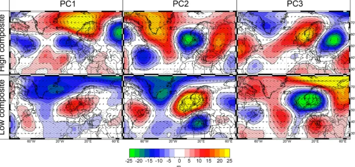
a complex temporally and spatially varying dataset by de- composing the dataset into fixed spatial patterns (EOFs) with corresponding time series (principle components, PCs), each representing a given proportion of the total variance in the dataset (Wilks, 2006). The magnitude of a given EOF loading gives the strength of the relation between the summer streamflow time series and the corresponding PC. A negative EOF loading represents an inverse relation between the summer streamflow time series and the corresponding PC, which can take on both negative and positive values. Mean summer (June–August) streamflows were computed for each year (1959–2018) and the time series standardised and detrended prior to the EOF analysis. The June–August period was chosen for the analysis (rather than May–August, which is in focus in Sect. 3.1–3.3) to avoid the effect of high flow in May caused by snowmelt. Furthermore, EOF analysis and composite maps are traditionally done on a 3-month seasonal basis, making the results more easily comparable to other studies. The EOFs and PCs were calculated using the Python libraryeofs(Dawson, 2016). For each of the principle components (PCs), years with absolute values larger than 1 standard deviation were defined as high (positive values) and low (negative values) anomaly years. For each set, we computed “high years composite maps” and “low years composite maps” of concurrent (mean summer; June–August) HGT500 anomalies. The significance of the composite maps was estimated by a two-sided t test at a 5 % significance level.

4 Results

4.1 Meteorological situation

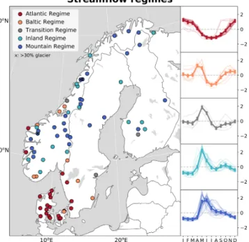
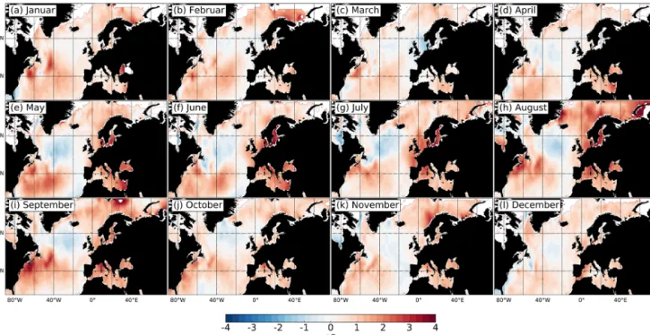
Figure 3a–d shows the evolution of SST anomalies from May to August 2018 as compared to the reference period (1971–

2000; all months throughout 2018 are shown in Fig. A1).

The strongest SST anomalies in the seas surrounding Europe in 2018 were found in May–September. Patterns of negative and positive SST anomalies were relatively stable from May to September, characterised by one negative and two positive anomalous SST centres. The strongest negative SST anomalies were found in an area south of Greenland (50–60^◦N), whereas strong positive SST anomalies were found below this area, in a belt from 20 to 80^◦W at approx. 40^◦N. A second region of positive SST anomalies was found in the regions surrounding Europe between 0 and 40^◦E (Barents Sea, Norwegian Sea, North Sea, Baltic Sea, Black Sea, and parts of the Mediterranean Sea). The highest SST anomalies exceeded 3^◦C and were found in the Baltic Sea.

HGT500 anomalies for each month (May–August 2018) as compared to the reference period (1971–2000) are shown in Fig. 3e–h (all months throughout 2018 are shown in Fig. A2). May 2018 was characterised by a dipole-like struc-

ture in the atmospheric circulation, with HGT500 anomalies ranging from −120 to 120 m. A high-pressure system (anticyclonic circulation) was centred over Fennoscandia, whereas Greenland and eastern Canada were under the influence of a low-pressure system (cyclonic circulation). This represents a northwestern movement of the high- and low- pressure systems present in April, when these were located over central or eastern Europe and the North Atlantic west of Ireland, respectively. South of the cyclonic circulation in May, a weaker anticyclonic circulation was observed over the east coast of the US. In June, the HGT500 anomalies were generally lower than in May, with anticyclonic conditions centred over the British Isles and at similar latitudes, with two cyclonic circulations: one centred over the Canadian east coast and one centred over Russia at approx. 70^◦E. The HGT500 anomalies in July were similar to the ones in May in their spatial patterns and anomaly magnitudes but with a slight northward shift. In August, the high-pressure systems weakened in magnitude, with a high-pressure system located southeast of Fennoscandia, and a low-pressure system developed over the North Atlantic between Iceland and Nor- way. Similar anomalous patterns and magnitudes persisted in September–October, before Fennoscandia again was under the influence of a strong high-pressure system in November and (too a lesser degree) December 2018.

The 2018 anomalies of the mean May–August HGT500 relative to 1959–2018 (represented as standard deviations, SDs, from the 60-year mean) for a sequence of subdomains in Europe are shown in Fig. 4a. Each subdomain covers 20^◦longitude×20^◦latitude. Results for each month (May–

August 2018) separately are shown in Fig. A3. Most of Eu- rope showed HGT500 anomaly values of more than 2 SDs, and in regions centred around Denmark (between 2.5^◦W and 12.5^◦E and between 52.5 and 57.5^◦N), HGT500 devi- ated by more than 3 SDs. Figure 4b shows the aggregated May–August HGT500 time series for a selected subdomain centred over Scandinavia (Scandinavian subdomain: 52.5–

72.5^◦N and 5–25^◦E), demonstrating a record-breaking high- pressure system over the period May–August for this subdomain. As shown in Fig. A3, particular high anomalies were observed in May and July, whereas more normal values were found in June and August. In May 2018, the SD was twice as high as the second most extreme year (1993) and more than 3 SDs away from the mean.

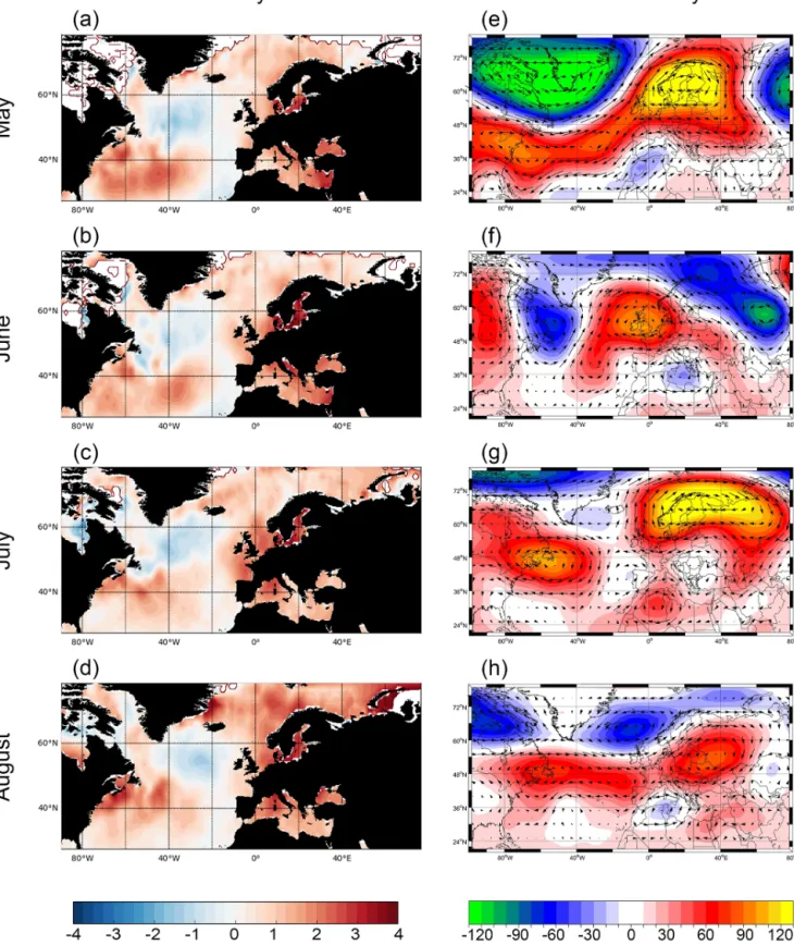
Figure 5a–d shows the top-six ranking of each month (May–August 2018) highest temperatures (all months throughout 2018 are shown in Fig. A4 and monthly anomalies in Fig. S1). Temperatures during this period were ex- ceptionally high, with record-breaking (rank 1) or near- record-breaking (rank 2–6) temperatures in several European regions. The most widespread extreme temperatures were found in May, when the top-six ranks (dominated by rank 1 and 2) covered almost the whole of the Nordic region and large parts of northern and eastern Europe. Record-breaking weather was reported by meteorological offices across the

(10)

Figure 3.Left panels: sea surface temperature (SST) anomalies for(a)May,(b)June,(c)July, and(d)August 2018 relative to the reference period (1971–2000). Right panel: geopotential height at 500 mbar (HGT500) anomalies for(e)May,(f)June,(g)July, and(h)August 2018 relative to the reference period (1971–2000). Zonal and meridional wind at the 500 mbar level are added to indicate wind directions.

(11)

S. J. Bakke et al.: The 2018 northern European hydrological drought and its drivers 5631

Figure 4. (a)Geopotential height at 500 mbar (HGT500) shown as standard deviation (SD) of aggregated May–August 2018 values based on the 60-year period (1959–2018) for subdomains of 20^◦longitude×20^◦latitude throughout Europe, shifted 2.5^◦at a time. The coloured squares are the centre points of each subdomain. This is illustrated for one subdomain over Scandinavia, with a large square and a small square marking the subdomain’s border and centre point, respectively.(b)Aggregated May–August HGT500 1959–2018 time series for the Scandinavian subdomain marked in(a).

affected countries. In Norway and Germany, for example, the meteorological institutes reported that the country average May temperature was the highest on (the more than 100-year) record, and 97 meteorological stations in Nor- way (with record lengths between 15 and 155 years) reg- istered record-breaking May temperatures (Grinde et al., 2018a; Deutscher Wetterdienst, 2018). In June, the area covered by extreme temperatures decreased, mainly covering a smaller region from northern France to Poland, southern Scandinavia, and the British Isles. Ireland stood out this month, with record-breaking temperatures. Only southern parts of Fennoscandia had ranks of 1–6 in June; however, this changed drastically in July, when almost the whole of Fennoscandia experienced the highest (or second highest) temperatures on the record. In Norway, 43 meteorological stations broke their mean July temperature record (Grinde et al., 2018b). High ranks were also seen in regions fac- ing the North Sea and the Baltic Sea. A southern shift was seen in August, when a southwest–northeastern belt of extreme temperatures extended from the Iberian Peninsula to southeastern Fennoscandia. Regions, mainly in Spain, Por- tugal, and Germany experienced record-breaking temperatures this month. Extreme temperatures were also observed in the months before and after May–August 2018 (mainly in April, September, and October), covering regions south of Fennoscandia. In November, temperatures in northern and western Fennoscandia were again extremely high.

Record-breaking (or near-record-breaking) low precipitation for each month (May–August; Fig. 5e–h; rank of all months are shown in Fig A5 and monthly anomalies in Fig. S2) were much less common and only found in smaller and more scattered areas across northeastern Europe. Some localised extreme clusters were found in June, mainly in southern UK, Benelux, Germany, and Belarus. In July, larger clusters were seen covering Benelux, Denmark, parts of Fennoscandia, and Germany. A relatively large region north of the Black Sea, including Moldova and parts of Roma- nia, Ukraine, and Russia, experienced record-breaking and near-record-breaking low precipitation in August. In addition, smaller clusters of extremely low August precipitation were found in central Europe. Apart from May–August, scatters of record-breaking or near-record-breaking low precipitation in 2018 were mainly found in southwestern, central and southeastern Europe. Exceptions are February and November, when larger parts of northern Europe experienced extremely low precipitation.

4.2 Meteorological drought

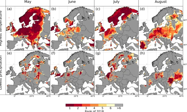
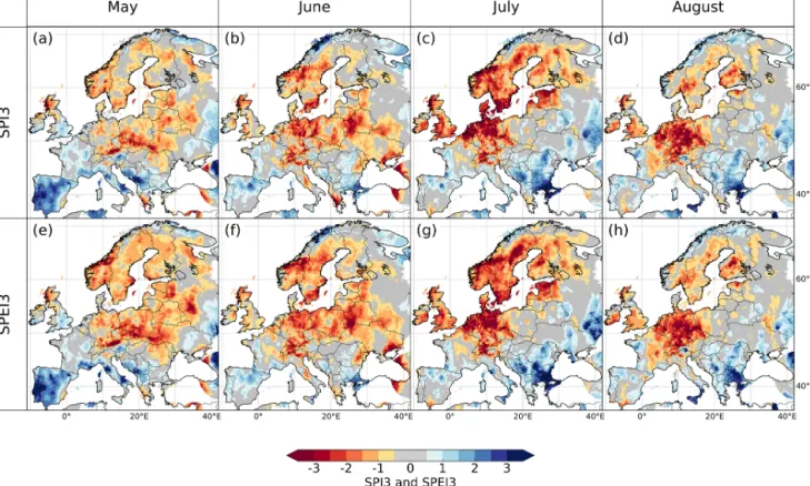
SPI3 and SPEI3 for each month (May–August 2018) are shown in Fig. 6 (all months are shown in Fig A6 for SPI3 and Fig A7 for SPEI3). From a slow development at the start of the year, a meteorological drought manifested itself (as indicated by SPI3<−1) across a larger region north of 45^◦N in April and May. The situation worsened to peak in July when 18 % of the grid cells had SPI3<−1.5. The most extreme

(12)

Figure 5.Top-six ranking of 2018 highest temperature (monthly mean of daily maximum temperature) for(a)May,(b)June,(c)July, and (d)August and top-six ranking of 2018 lowest precipitation for(e)May,(f)June,(g)July and(h)August. Analysed period is 1959–2018.

A rank of 1 signifies that 2018 had the warmest (in the case of temperature) or driest (in the case of precipitation) month since 1959, a rank of 2 signifies that 2018 had the second most extreme value in that month, etc.

meteorological drought in northern Europe (SPI3<−2) was found in July in a region surrounding Denmark, including southern Norway, Sweden, Benelux, and Germany. Regions within the British Isles and the Baltic countries also recorded extreme meteorological drought this month. In August, extreme conditions persisted in Germany and neighbouring countries, whereas the meteorological drought in Fennoscan- dia, the Baltic countries, and the British Isles generally less- ened (or ceased). Dry conditions persisted in central Eu- rope, and extended to southern and eastern parts of Europe in September–November. Eastern and southeastern parts of Fennoscandia were again affected by moderate drought in November–December after 3 months of only scatters of moderate drought in this region.

The year started rather wet across Europe in terms of SPI3, with wet conditions persisting in southeastern Eu- rope until May. SPI3 also revealed extreme wet conditions (SPI3>2) on the fringe of the drought-affected area, i.e.

along the coastal regions in northern Norway (June–October) and southern parts of Europe, notably the Iberian Peninsula (March–May) and southeastern Europe (February–April and July–August). The SPEI3 showed a similar spatial pattern as SPI3, although somewhat higher anomalies were seen in May and June for SPEI3, with 11 % and 16 % of the grid cells

in severe or extreme drought (i.e. values<−1.5) as compared to 7 % (May) and 13 % (June) for SPI3, respectively.

4.3 Hydrological drought

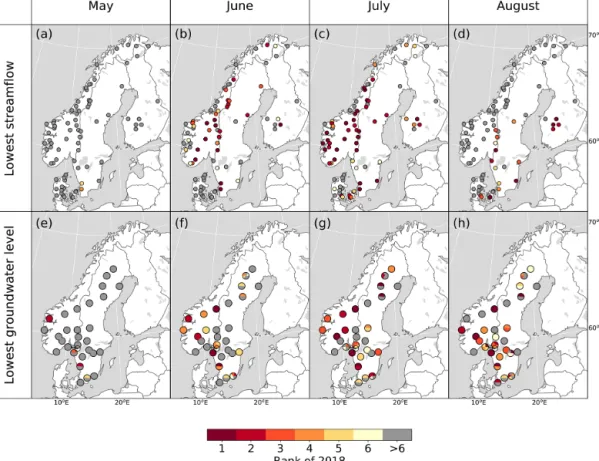
The 60-year (top-six) ranking of lowest monthly streamflow in 2018 in the Nordic region (Norway, Sweden, Finland, and Denmark) revealed record-breaking or near-record-breaking low streamflow in several regions from June, peaking in July (Fig. 7a–d). Ranks of all months in 2018 are shown in Fig. A8, and standardised monthly hydrographs for 2018 are shown in Figs. S3–S5. In May, only two (3 %) of the stations experienced extremely low streamflow (rank of 1–6).

In June, however, 46 % of the stations had extremely low streamflow and 13 % were record breaking. The proportion of stations with extremely low streamflow expanded to 68 % in July (28 % were record breaking). Extreme conditions persisted in the southeastern area of the region (mainly eastern Denmark, southeastern Sweden, and southern Finland) until the end of the year.

The 30-year (top-six) ranking results of lowest monthly groundwater levels in Sweden and Norway for each month (May–August 2018) are shown in Fig. 7e–h (all months are shown in Fig A9, and monthly standardised groundwater ta-

(13)

Figure 6.Meteorological drought 2018 indexed by SPI3 for(a)May,(b)June,(c)July, and(d)August, and SPEI3 for(e)May,(f)June,(g) July, and(h)August. Reference period used is 1971–2000.

bles can be found in Figs. S6 and S7). Four (7 %) of the stations in Norway and Sweden had extremely low groundwater levels (rank of 1–6) in May 2018. In June, 43 % of the stations had a rank of 1–6 (7 % were record breaking), ex- panding to 55 % (14 % record breaking) in July and 63 % (14 % record breaking) in August. Ranks between 1 and 6 were seen in 38 %–54 % of the wells until the end of 2018.

Extremely low groundwater levels did not show any distinct spatial patterns. In several cases, stations located close to each other (pies of the same point) showed different results, reflecting the importance of local conditions in determining the groundwater level.

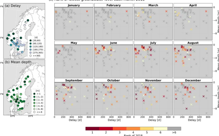
The delay in groundwater response to precipitation (as defined in Sect. 3.3) varied among the study sites from 30 to 1500 d (Fig. 8a), whereas mean groundwater levels (measured from the surface) ranged from 0.36–13.4 m (median of 2.16 m; Fig. 8b). With one exception, the most extreme groundwater levels in Norway in June and July 2018 (in terms of ranks) were found for locations with the fastest response time, i.e. 30–90 d. Figure 8c shows the top-six groundwater ranks for each month throughout 2018 plotted with the response delay along thex axis and the mean groundwater level depth (Fig. 8b) along theyaxis. Extreme groundwater levels emerged in June in the most shallow wells (less than 3 m depth from surface), followed by deeper wells in July–August, with response delays of up to 400 d. In

September, the most shallow wells with the fastest response showed less extreme ranks, whereas deeper and more slowly responding wells started to experience extreme conditions.

This pattern continued throughout 2018.

4.4 Relation between summer streamflow and large-scale atmospheric circulation

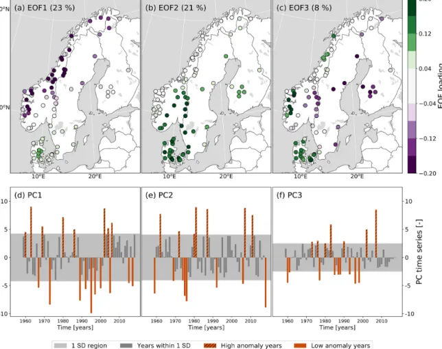
The first three principle components of the EOF analysis explained 52 % of the detrended and standardised summer streamflow variability over the period 1959–2018, and their time series and loadings are shown in Fig. 9. EOF1 explained 23 % of the variability and was mostly relevant for the streamflow in the western and northern part of Norway (Fig. 9a). EOF1 was also relevant for some stations in Den- mark, which were characterised by high flow when stations in Norway had low flow and vice versa. In summer 2018, PC1 was close to 1 standard deviation higher than the time series mean (Fig. 9d), reflecting dry conditions in western and northern Norway. Similar to EOF1, EOF2 explained 21 % of the summer streamflow variability (Fig. 9b). EOF2 was mostly relevant for the streamflow in Denmark, southeastern Norway, and southwestern Sweden. The PC2 time series indicated extreme low flow conditions in summer 2018 in these regions (Fig. 9e). A smaller amount of variability (8 %) was explained by EOF3 (Fig. 9c). EOF3 reflected op-

(14)

Figure 7.Top-six ranking of lowest streamflow for(a)May,(b)June,(c)July, and(d)August, and top-six ranking of 2018 lowest groundwater level for(e)May,(f)June,(g)July, and(h)August. Analysed period is 1959–2018 for streamflow and 1989–2018 for groundwater. A rank of 1 signifies that 2018 had the lowest monthly streamflow (upper panels) or groundwater level (lower panels) since the beginning of the analysed period; a rank of 2 signifies that 2018 had the second most extreme value in the given month, etc.

posite summer streamflow conditions in the west (Norway and Denmark) relative to the east (easternmost Norway, Swe- den, and Finland). The PC3 value for 2018 was close to the time series mean (Fig. 9f); thus, the conditions represented by EOF3 and PC3 were not relevant for the summer 2018.

Summers of low and high streamflow were related to the prevailing large-scale atmospheric circulation by extracting the summer HGT500 of low and high anomaly years from the first three PC time series from the summer streamflow EOF analysis. Years with absolute PC values larger than 1 standard deviation from the times series mean were defined as high (positive values) and low (negative values) anomaly years. Summer (June–August) HGT500 composites for these years, along with wind directions and significance, are shown in Fig. 10.

Summer low flow in western and northern Norway, as indicated by high PC1 values, was associated with a high- pressure system centred over the Norwegian Sea and covering most of Fennoscandia and a low-pressure system centred over the British Isles and over Russia at approx. 60^◦E. In summers with low PC1 values, western and northern parts of Fennoscandia were located on the border between a low-

pressure system in the north and a high-pressure system in the south. Years of high (low) PC2 values were associated with a low-pressure (high-pressure) system over the North Sea, flanked by a high-pressure (low-pressure) system on the central part of the North Atlantic and over Russia. These pressure systems covered the region with the largest EOF2 loadings, with summer high flow associated with cyclonic circulation and summer low flow associated with the an anticyclonic circulation over the region. A high-pressure system centred over southern Scandinavia and a low-pressure system over Russia at approx. 40^◦E were observed for summers of high PC3 values, and a low-pressure system over the North Sea and southern Scandinavia was observed for summers with low PC3 values.

5 Discussion

The 2018 extreme drought centred in northern Europe sub- stantially affected the Nordic region, particularly in late spring and summer, before moving southwards in August.

The Nordic region has widely different hydroclimatological and terrestrial characteristics as compared to other recently

(15)

Figure 8. (a)Delay in groundwater response to precipitation,(b)mean 1989–2018 groundwater depth below surface, and(c)top-six ranking of lowest groundwater level in each month of 2018 plotted with each well’s delay and mean depth along thexaxis andyaxis, respectively.

Two wells, one with delay of 1500 d and one with mean depth of−13.4 m, are outside the range of the ranking plots. Those two wells had no rank of 1–6 in April–December 2018.

drought-affected regions, such as southern and central Eu- rope in 2003 and 2015. This makes the drought of 2018 and its propagation in the hydrological cycle unique. Spe- cial for the region is a high diversity in hydroclimatological conditions, including the effect of snow on hydrology. Ac- cordingly, the response to a meteorological drought and its propagation in the hydrological cycle will vary. Here, we dis- cuss the 2018 drought, first from a climatological perspective (Sect. 5.1) and then by considering its hydrological footprint (Sect. 5.2). Further, the results of the EOF analysis, linking atmospheric circulation and low summer streamflow in the Nordic region, are discussed (Sect. 5.3), followed by some final remarks on the representativity of the hydrological data used in the study (Sect. 5.4).

5.1 The 2018 drought from a climatological perspective The 2018 drought confirmed the central role of anticyclones in the development of northern (>40^◦N) Eurasian droughts as highlighted by Schubert et al. (2014). The strongest HGT500 anomalies over the period May–August were found in May and July. May was characterised by a cyclonic circulation centred over Greenland and western Russia and pro-

nounced anticyclonic circulation centred over the continental Nordic region, extending south to central North Atlantic and the east coast of North America. This wave train pattern resembles the atmospheric circulation associated with the leading mode of drought variability over Europe as presented by Ionita et al. (2015). Large parts of the region expe- riencing anticyclonic conditions in the months from May to August 2018 also showed extreme temperatures (defined as having a rank between 1 and 6). The stronger the HGT500 anomaly, the more extreme the temperature, emphasising the strong link between the two variables.

Overall, the observed positive SST anomalies in summer 2018 overlapped spatially with the anticyclonic circulation (positive HGT500 anomalies) in May and July 2018.

Anomalous anticyclonic circulation, as observed in these two months, decrease convection and increase incoming solar radiation, leading to warmer SST in the underlying seas (Feu- dale and Shukla, 2011). The spatial pattern of SST anomalies in 2018 are similar to those in the summers of 2003 and 2015, representing two of the most extreme drought events in Europe in recent years (Ionita et al., 2017; Laaha et al., 2016; Fischer et al., 2007b; Black et al., 2004). During all three events, a persistent negative anomaly was centred south

(16)

Figure 9.Empirical orthogonal function (EOF) analysis based on aggregated summer (June–August) standardised and detrended streamflow (1959–2018). Maps(a–c)show the EOF loadings; time series(d–f)show the first three principle components (PCs). The explained variability of each mode is given in brackets in the corresponding EOF plot. For each of the PCs, years with absolute values larger than 1 standard deviation (SD) are highlighted as high (positive values) and low (negative values) anomaly years.

of Greenland over the period May–August. The anticyclonic centres and associated temperature extremes over continental Europe in 2018 were generally located more towards the northeast as compared to the 2003 and 2015 events. An over- lapping region in central Europe experienced temperature extremes all three summers. Overall, most major European streamflow droughts between 1960 and 1990 were associated with high-pressure systems across central Europe (Stahl, 2001), highlighting the unique location of the 2018 event.

This is especially the case for May and July, when the high- pressure system centred over the Nordic region was more than 3 SDs and 2 SDs, respectively, away from the 60-year mean (Fig. A3). However, in August 2018, the region of extreme temperature moved southeast, covering a region extending from the southwest to northeast Europe, resembling the affected region in summer of 2015 (and to a lesser degree 2003).

Monthly precipitation extremes during the period May–

August were not as widespread as temperature extremes;

however, areas with extreme low precipitation (rank between 1 and 6) generally also experienced extreme high temperatures. Overall, the region affected was located further north as compared to previous large-scale droughts in Europe, such as the summer droughts in 2003 and 2015 (Ionita et al., 2017). The SPI3 and SPEI3 both showed similar northern European located dry anomalies. These indices both reflect a 3-month accumulated deficit (in precipitation and a climatic water balance, respectively); thus, a higher consistency is seen in time. Furthermore, both indices showed widespread dry conditions already in April, reflecting conditions in the months February–April. As seen in Fig. A4, extreme high temperatures were seen already in April in large parts of Eu- rope, which potentially led to drier-than-normal conditions in the soils.

For both SPI3 and SPEI3, the spatial extent of severe and extreme drought peaked in July. Overall, the percentage of grid cells showing extreme drought was higher for SPEI3, highlighting the importance of not just looking at precipita-

(17)

Figure 10.Composite maps of summer (June–August) geopotential height at 500 mbar (HGT500) anomaly relative to 1971–2000 for the first three PCs. High and low composites maps are shown, representing years with (positive and negative) values more extreme than 1 standard deviation in the corresponding PC time series.

tion when analysing the impact of drought, as already recog- nised by Stagge et al. (2017). The use of potential evapotranspiration in SPEI (rather than actual evapotranspiration) may be less an issue in the Nordic region where evapotranspiration in general is limited by energy, as opposed to water-limited areas dominating in central and southern Eu- rope (McVicar et al., 2012). The inclusion of potential evapotranspiration in SPEI (as opposed to using only precipitation in SPI) may therefore prove acceptable for drought assessments in energy-limited regions. However, water may be- come a limiting factor in these regions in exceptional years, such as the summer of 2018 (Buitink et al., 2020). As the soil dries out, it may give rise to a positive land–atmosphere feedback, i.e. an enhanced warming is seen as less energy is spent on evapotranspiration. Such soil-moisture–temperature feedbacks have played an important role in the evolution of previous European heat waves (Fischer et al., 2007a), and it may have played an important role in the 2018 event as well.

Being outside the scope of this study, this would be an inter- esting aspect of a further study.

5.2 The 2018 drought from a hydrological perspective Overall, drought impacts are commonly related to deficits in different components of the hydrological cycle and not in the meteorological variables as such. Key impacts of the 2018 drought were related to soil moisture (crop failure and wild fires) and hydrological drought (e.g. impacts on energy, water supply and aquatic ecosystems). As a drought propagates, the event is normally lagged, attenuated, and lengthened as

compared to the original meteorological event (Van Loon and Van Lanen, 2012; Van Loon et al., 2011). The degree to which this happens varies with event and region impacted.

Furthermore, antecedent water storage (initial conditions), such as snow, glaciers, and groundwater, plays an important role in the occurrence, timing, and development of a hydrological drought.

In regions affected by seasonal snow, drought occurrence and propagation is to a large degree influenced by the snow volume and snowmelt timing as compared to a normal year.

During the snow accumulation season in 2018, above-normal precipitation fell in early winter in most of the Nordic region, and less-than-normal precipitation occurred in western and northern Norway and Finland towards the end of the snow season (as indicated by SPI3; Fig. A6a–c). Most of the snow-dominated catchments (with the exception of the northernmost part of the Nordic region) experienced meteorological drought in May–July. Record high temperatures emerged during the snowmelt season (i.e. in May) and 19 stations (24 %), all with a Mountain or Inland regimes, experienced one of their six highest May streamflow since 1959.

For other stations affected by snowmelt, however, a more normal flood situation followed (Figs. S4 and S5); one hy- pothesis is that part of the snow was lost due to sublimation.

In addition, higher-than-normal evapotranspiration rates led to less water feeding the streams. The high snowmelt and evapotranspiration rates likely caused an earlier end of the snowmelt season as well as a smaller total volume of meltwa- ter contribution to streamflow compared to normal (given the same preconditions). Following the snowmelt peak, stream-

(18)

5638 S. J. Bakke et al.: The 2018 northern European hydrological drought and its drivers flow drought started emerging in June in large parts of the

Nordic region. Noteworthy exceptions were the three glacier- dominated streamflow stations (Fig. S5), for which high summer temperatures led to high melt rates and sustained water contribution from the glaciers.

Streamflow stations without a snow season are mainly located in Denmark and southern Sweden. Extreme temperatures were found in part of this region already in April, extending to the whole region in May. In southern Sweden, meteorological and hydrological drought developed from May, and record-breaking low streamflow was seen from June.

Most of Denmark, on the other hand, did not experience a meteorological drought until July. Accordingly, streamflow drought was first observed in July and (to a lesser degree) August. However, this was only seen for stations located in the southeastern parts of Denmark. Stations in western and northern Denmark did not experience extremely low streamflow at all during May–August 2018. As a whole, Denmark had extremely low precipitation and severe-to-extreme meteorological drought, as indicated by SPI3, in July. However, a southeastern–northwestern gradient in extreme temperature (and SPEI3) reflects the spatial pattern of extremely low streamflow in Denmark this month, indicating that higher- than-usual evapotranspiration rates likely contributed to extreme conditions in the southeast. Correspondingly, less extreme evapotranspiration in the west and north might have prevented streamflow drought to develop there.

Whereas extremely low streamflow conditions sustained in the southeastern area of the Nordic region (southeastern Denmark, southeastern Sweden, and southern Finland) throughout 2018, streamflow in the north and western part of the region was replenished by high precipitation totals in August (Fig. S2h). This divide reflects the southeastern movement of the anticyclonic circulation as well as the cyclonic circulation over the Norwegian Sea in August, with winds from the North Sea bringing precipitation towards the coast. High precipitation totals between August and Octo- ber did not only replenish the rivers and end the streamflow drought but also led to extremely wet conditions at several streamflow stations (Figs. S3–S5). Western and northern stations experienced one of their six highest monthly streamflows since 1959 in August (5 stations), September (21 stations), and October (16 stations). In the southeastern area, extreme streamflow conditions persisted towards the end of 2018. Extreme conditions reappeared in November, even affecting stations that did not experience extremely low streamflow during the summer. This can be explained by continued below-normal precipitation in September–October (Fig. S2) and a new high-pressure system over northeastern Europe in November, leading to extremely low precipitation and severe to extreme meteorological drought in large parts of the southeastern Nordic region.

The groundwater wells were all located in areas affected by moderate-to-extreme meteorological drought, as indicated by SPEI3, in May, June, July, and (to a lesser degree) Au-

gust. The high spatial variability in hydrogeological prop- erties across the Nordic region is mirrored in the diversity in groundwater response to meteorological conditions, as reflected in a high local variability for groundwater drought (rank between 1 and 6) even for closely located wells. Ex- cept for four wells that experienced low groundwater levels already from March, no wells showed groundwater drought in May. Similar to streamflow, this was likely due to wet preconditions, such as high groundwater levels and/or snow volumes recharging groundwater during the melt season (Figs. S6 and S7). In June, extreme conditions were found among the most shallow groundwater wells, probably due to high evapotranspiration rates in combination with precipitation deficits. From July onwards, extreme conditions were found in wells of increasing depth and response time. The extreme conditions first started to cease in the shallowest and fast responding wells from September. At the end of the year, 38 % of the wells still experienced extreme conditions, and below-normal groundwater levels persisted well into 2019 (e.g. Table 1n). Similar to streamflow, this was likely a combined effect of a delay in the hydrological system, a continued below-normal precipitation and meteorological drought associated with a high-pressure system es- tablishing over northeastern Europe in November.

5.3 Atmospheric circulation associated with low summer streamflow in the Nordic region

The EOF analysis revealed that more than half (52 %) of the variability in summer streamflow in the Nordic region (1959–

2018) can be explained by the first three principle components, whereof the first two EOFs explained 44 % (Fig. 9).

The analysis was somewhat biased towards Danish conditions, as the station density was much higher there compared to the rest of the region, in particular Sweden and Finland. EOF1 and EOF2 indicated two distinct patterns in summer streamflow variability: in western and northern Nor- way (EOF1) and in the southeastern part of the Nordic region (EOF2). During 1959–2018, low summer streamflow in the whole region only occurred twice, i.e. 1969 and 2006.

These summers have also previously been identified as ex- ceptionally dry by different drought indices (e.g. Spinoni et al., 2015; Hannaford et al., 2011) and here found to correspond to May–August HGT500 anomalies of more than 1 SD above the 1959–2018 mean (Fig. 4).

High values of summer PC1 indicated low summer streamflow in the northwestern part of the Nordic region, and were associated with a high-pressure system over the Norwegian Sea (Fig. 10). Several of the streamflow stations with strong EOF1 loadings recorded extremely low streamflow values in June and July 2018. However, the summer of 2018 was not a high anomaly year in PC1, which might be due to the high precipitation in August 2018 replenishing the rivers.