Belyi pairs and scattering constants

(1)

Belyi pairs and scattering constants

D I S S E R T A T I O N

zur Erlangung des akademischen Grades Dr. rer. nat.

im Fach Mathematik eingereicht an der

Mathematisch-Naturwissenschaftlichen Fakultät II Humboldt-Universität zu Berlin

von

Dipl.-Math. Anna Elisabeth Posingies 8. September 1980, Berlin

Präsident der Humboldt-Universität zu Berlin:

Prof. Dr. Dr. h.c. Christoph Markschies

Dekan der Mathematisch-Naturwissenschaftlichen Fakultät II:

Prof. Dr. Peter Frensch Gutachter:

(i) Prof. Dr. Jürg Kramer (ii) Prof. Dr. Ulf Kühn

(iii) Prof. Dr. Jürgen Wolfart eingereicht am: 25. Mai 2010

Tag der mündlichen Prüfung: 14. September 2010

(2)

(3)

Abstract

In this dissertation non-holomorphic Eisenstein series and Dessins d’Enfants are considered. Non holomorphic Eisenstein series are created out of subgroups of the modular group by summing up over all elements modulo the stabilizer of a cusp.

The second main object, Dessins d’Enfants, are bipartite graphs that are embedded into topological surfaces.

There is a correspondence between Dessins D’Enfants, Belyi pairs (a non-singular algebraic curve with a map toP¹ramified above at most three points) and subgroups Γ ⊂ Γ(2) of finite index. Therefore Eisenstein series and Dessins d’Enfants are related and a focus of this work is how to use the one to find information about the other.

The main results concerning Dessins d’Enfants in this thesis are investigations of symmetries of Dessins.

We have been able to interpret automorphisms of algebraic curves on the associated Dessin, the subgroups and in particular the sets of cusps. Furthermore, we describe the relation of Dessins for subgroups Γ ⊂ Γ⁰ ⊂ Γ(2). Therefore, with help of the Dessins we can decide if two subgroups are contained in each other.

Together with our results on the Dessins for principal congruence subgroups this leads to an implemented algorithm that checks if a subgroup is a congruence subgroup or not.

On the side of Eisenstein series we consider scattering constants, Green’s functions and Kronecker limit formulas.

We found symmetries in the scattering matrix for certain groups. For Green’s functions we established a trace formula. We showed that Eisenstein series fulfill an identity we call Kronecker limit formula in which they are compared with functions coming from certain modular forms. Then combining the Kronecker limit formula with our trace formula allows us to determine scattering constants for particular subgroups.

Most of the work done in this thesis culminates in the calculation of the scattering constants for the Fermat curves. Concerning this result, one has to note that for nearly all N ∈ N the subgroup associated to the N-th Fermat curve is non-congruence.

(4)

(5)

Zusammenfassung

Diese Dissertation behandelt nicht-holomorphe Eisensteinreihen und Dessins d’Enfants. Nicht-holomorphe Eisensteinreihen entstehen aus Untergruppen der Mo- dulgruppe, indem man über alle Elemente der Gruppe modulo dem Stabilisator einer Spitze aufsummiert. Die zweite Struktur, Dessins d’Enfants, sind bipartite Graphen, die in topologische Flächen eingebettet sind.

Dessins d’Enfants stehen in Korrespondenz zu Belyi-Paaren (einer nicht-singulä- ren algebraischen Kurve mit einem Morphismus nachP¹, der nur über höchstens drei Punkten verzweigt ist) und Untergruppen Γ ⊂Γ(2) von endlichem Index. Deshalb bestehen zwischen Eisensteinreihen und Dessins d’Enfants Verbindungen und ein Schwerpunkt dieser Arbeit ist es, Informationen und Wissen über das eine Objekt in das andere zu übertragen.

Bezüglich Dessins d’Enfants beschäftigen wir uns mit Symmetrien.

Wir waren in der Lage, Automorphismen von algebraischen Kurven im assoziierten Dessin, in der zugehörigen Untergruppe sowie insbesondere auf den Spitzen zu in- terpretieren. Außerdem beschreiben wir die Zusammenhänge zwischen Dessins für Untergruppen Γ⊂Γ⁰⊂Γ(2), dadurch können wir für zwei Untergruppen anhand ih- res Dessins entscheiden, ob sie in einander enthalten sind. In Kombination mit hier erbrachten Resultaten zu den Hauptkongruenzuntergruppen führt dies zu einem im- plementierten Algorithmus, der prüft, ob eine Gruppe eine Kongruenzuntergruppe ist oder nicht.

Auf der Seite der Eisensteinreihen untersucht dieser Text Streukonstanten, Green- sche Funktionen und Kroneckergrenzformeln.

In der Streumatrix fanden wir Symmetrien (für bestimmte Gruppen). Für Green- sche Funktionen wurde eine Spurformel bewiesen. Wir zeigten, dass Eisensteinreihen eine Identität erfüllen, die wir Kroneckergrenzformel nennen. Dabei wird der kon- stante Term der Eisensteinreihe mit Funktionen verglichen, die von ausgezeichneten Modulformen kommen. Indem wir die Grenzformel mit der Spurformel verbinden, konnten wir Streukonstanten für gewisse Untergruppen ausrechnen.

Die Dissertation gipfelt in der Berechnung der Streukonstanten für die Fermatkur- ven. Bezüglich dieses Ergebnisses ist zu beachten, dass für die meistenN ∈Ndie zur N-ten Fermatkurve assoziierte Untergruppe eine Nichtkongruenzuntergruppe ist.

(6)

(7)

Introduction

The topics of this dissertation are non-holomorphic Eisenstein series on the one hand and Dessins d’Enfants on the other. These two objects are related and a focus of this work is to find out how to use the one to find information about the other.

Non-holomorphic Eisenstein series are created out of subgroups of the modular group by summing up over all elements modulo the stabilizer of a cusp. Hence, in these series the information of the subgroup is encrypted. They are eigenfunctions of the hyperbolic Laplacian and play a central role in spectral theory. Eisenstein series had first been introduced by H. Maass [Maa49]. In this thesis we will use the definition presented by T. Kubota [Kub73]. In this text the focus lies on one special term of the Eisenstein series, the constant term and the scattering matrices together with scattering constants, which are special values of scattering matrices, that can be derived from them. Scattering matrices for automorphic forms were treated by P. Lax and R. Phillips [LP67] with physical motivation. U. Kühn [Küh05] realized that scattering constants play a role in arithmetic intersection theory. For the Green’s functions derived from Eisenstein series used by U. Kühn, we established a trace formula (Proposition 4.2.8). In Proposition 4.3.5 we showed that Eisenstein series fulfill an identity we call Kronecker limit formula.

Then combining the Kronecker limit formula with our trace formula allows to determine scattering constants for particular groups (Propositions 4.3.8 and 4.3.10).

We can divide the subgroups of the full modular group Γ(1) into groups of two different kinds. On the one hand side are the congruence subgroups, groups such that all matrices whose entries fulfill certain congruence conditions are contained in them. On the other side there are non-congruence subgroups. The scattering matrices for congruence subgroups are essentially known, see D. Hejhal [Hej83] and M. Huxley [Hux84]. Results for non-congruence subgroups had hardly been found. A.B. Venkov [Ven90] worked with cy- cloidal non-congruence subgroups. He uses the fact, that the scattering matrix changes in a known way, if a subgroup has the same number of cusps than the supergroup. In general, there is a strong relation between the scattering matrix of a group and the ones of subgroups. This has been studied of the thesis of C. Keil [Kei06] and the Diplomarbeit of the author A. Posingies [Pos07]. The relations of scattering matrices have implications to scattering constants. These symmetries of scattering constants have been studied in this thesis (see Propositions 3.2.6, 3.3.3 and Conjecture 3.3.4). One main result is the calculation of the scattering constants for Fermat curves (Theorem 5.4.8); concerning this result, one has to note that for nearly all N ∈ N the subgroup associated to the N-th Fermat curve is non-congruence.

The first problem concerning non-congruence subgroups is to find a description of a subgroup with whom we can work. There exist several constructions for non-congruence subgroups (e.g. in [Ven90]). To check that the group received is non-congruence, most

(10)

Introduction

of the constructions make use of known properties concerning the widths of cusps and the index of the subgroup. Another possibility is to take any subgroup and test if it is congruence or not. Congruence test for subgroups given in special forms has been developed e.g. by T. Hsu [Hsu96] as well as by M.-L. Lang, C.H. Lim and S.-P. Tan [LLT95].

In Section 2.4 we present a new algorithm (Algorithm 2.4.2) to test if a subgroup Γ⊂Γ(2) is congruence. The algorithm is implemented in Maple (in Appendix A.2 together with A.1).

The second main object are Dessins d’Enfants. They are bipartite graphs that are embedded into topological surfaces. The name was given by A. Grothendieck [Gro97]

because of their simple appearance. The motivation to study such objects grew after G. Belyi [Bel79] published a result that connects Dessins with algebraic curves defined over number fields. Dessins are a description of covers ofP¹, that are only ramified in at most three points. G. Belyi showed that such covers exist for all non-singular algebraic curves defined over a number field. Beside that, Dessins define subgroups of Γ(2), since Γ(2)∼= Π₁(P¹(C)\ {3 points}). Therefore, one can study fundamental properties of such subgroups via Dessins d’Enfants. In the last thirty years, Dessins d’Enfants have been studied by many mathematicians with different aims. A prominent role takes e.g. the study in regard to the action of the absolute Galois group (see e.g. [SL97] and [Sch94]).

The main results concerning Dessins d’Enfants in this thesis are investigations of symmetries of Dessins.

We have been able to interpret automorphisms of algebraic curves on the associated Dessin, the subgroups and in particular the sets of cusps (Propositions 2.1.9 and 2.1.11).

Furthermore, in Theorem 2.3.1 we describe the relation of Dessins for subgroups Γ ⊂ Γ⁰ ⊂Γ(2). Therefore, with help of the Dessins we can decide wether two subgroups are contained in each other or not.

Together with results on the Dessin for principal congruence subgroups (Theorem 2.2.4) this leads to the algorithm (Algorithm 2.4.2) already mentioned.

In the following, we will present the content of this dissertation in detail.

In Chapter 1 Dessins d’Enfants are treated. We start by defining Dessins and giving some equivalences: Belyi pairs, Belyi permutations, subgroups of the modular group and Dessins are in correspondence to each other. In Section 1.2 we give a sketch of the proof of these equivalences.

In the rest of Chapter 1, we will present some properties and details concerning the Belyi equivalences.

At first, in Section 1.3, we study the relation of Dessins and the Belyi permutations. In particular, we show how to construct σ∞, the Belyi permutations for the faces of the Dessin, without usingσ0 and σ1. After that in 1.4, we give an explicit description of the correspondence of cusps of the Belyi pair and the associated subgroup (Theorem 1.4.6).

Section 1.5 is devoted to the full Dessin, a variation of Dessin d’Enfants that allows to see more of the structure of the Belyi pair. Finally, Section 1.6 gives a description how to calculate the Dessin for a subgroup Γ⊂Γ(2). So far, we only considered the inverse problem to get the subgroup out of a Dessin.

(11)

Introduction After this repetition, in Chapter 2 we come to new results.

In Section 2.1, we study how automorphisms of an algebraic curve (with Belyi map β) translate to the associated subgroup. We restrict the examination to automorphisms that map the full Dessin, i.e. β⁻¹(R), to itself. The result is that such automorphisms induce automorphisms on the associated subgroup given by exchanging and possibly inverting the generators of Γ(2) plus a conjugation (Proposition 2.1.9). The conjugation is not uniquely determined but all this automorphisms induce the same action on the cusps (Proposition 2.1.11).

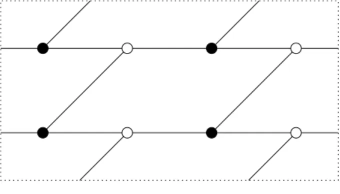
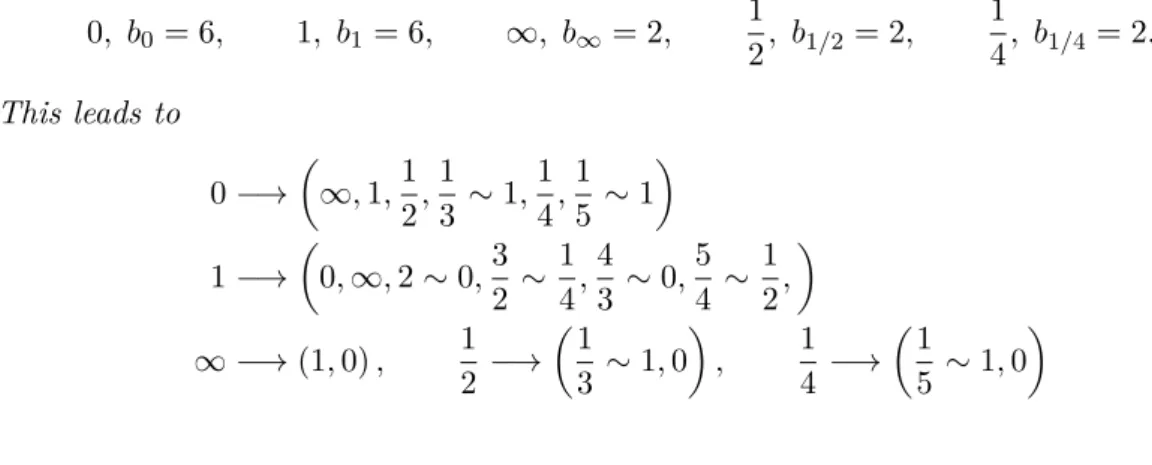
The next part, Section 2.2, deals with the Dessins for principal congruence subgroups Γ(N) for evenN. See for example Figure 0.1 on page 3 for the Dessin for Γ(6). This is a Dessin of genus 1, i.e. opposite sides in the figure have to be identified.

Figure 0.1.: Dessin for Γ(6)

We have been able to develop an algorithm (in Theorem 2.2.4) that calculates the Belyi permutations for Γ(N). A Maple implementation of it can be found in Appendix A.1.

After that, in Section 2.3, we discuss the question how to distinguish Dessins of subgroups Γ ⊂Γ⁰ ⊂Γ(2). The solution of this problem is that the fact Γ⊂Γ⁰ translates into the existence of a map from the set the Belyi permutations of Γ act on into the set where the Belyi permutations of Γ⁰ act on (Theorem 2.3.1). With this result we can construct new subgroups of arbitrary index for a given group Γ⁰. In Algorithm 2.3.4 the construction is explained and we give two examples. Another possible application for that result is to answer the question if a group is a congruence subgroup. We combine the results of the Sections 2.2 and 2.3 in Section 2.4. That yields an implemented algorithm (Algorithm 2.4.2 and Appendix A.2) that decides if a subgroup given by Belyi permutations is congruence.

In the third chapter, we concentrate on Eisenstein series and scattering constants. For each cusp Sj of a finite index subgroup Γ⊂Γ(1) we have an Eisenstein series E_j^Γ(z, s) from whose expansion in a cusp S_k we can derive the scattering constant C_jk^Γ. After the basic definitions and properties in Sections 3.1 and 3.2 we consider sum relations of Eisenstein series and scattering constants. Most of it bases on Proposition 3.1.7 (originally from [Pos07]). A generalized formula for sums of scattering constants is presented in Proposition 3.2.6.

(12)

Introduction

In Section 3.3 we recall the results from Section 2.1 about automorphisms of Dessins.

Calculations of some examples imply that automorphisms lead to identities of scattering constants (Conjecture 3.3.4): For an automorphism of a Belyi pairα:C→C we expect

C_jk^Γ =C_α(j)α(k)^Γ

for the associated subgroup Γ and the induced morphism on the cusps. We could proof that formula only in a special case, when α : Γ → Γ is given by conjugation only (Proposition 3.3.3).

Chapter 4 continues working with Eisenstein series. Here, the focus lies on Green’s functions g_j^Γ(z) derived from Eisenstein series and Kronecker limit formulas for them.

By subtracting the pole, we can define (log-log singular) Green’s functions for the cusps.

They fulfill the following identities for Γ ⊂Γ⁰ ⊂Γ(2) with cusps S_k (for both groups) andS_j^Γ⁰ =^S_i∈I

jS_i^Γ; theb’s denote the widths in Γ, the w’s the widths in Γ⁰ X

i∈Ij

bi

w_jg_i^Γ(z) =g^Γ_j⁰(z), as shown in Proposition 4.2.5 and

Tr_Γ|Γ0

g^Γ_j(γ_kz)=g^Γ_j⁰(γ_kz) (Proposition 4.2.8). This is content of Section 4.2.

In Section 4.3 we show that Eisenstein series fulfill Kronecker limit formulas for distinguished modular formsfj and A∈R(Proposition 4.3.5):

4πlim

s→1

E_j^Γ(z, s)− 1 vol(Γ)(s−1)

=−log||f_j||²+A.

With the summation formulas for Green’s functions we can establish Kronecker limit formula (Proposition 4.3.10) and then calculate scattering constants (Proposition 4.3.8).

In the last section 4.4 the Green’s functions (Theorem 4.4.6) and Kronecker limit formulas (Proposition 4.4.12) for the group Γ(2) are presented.

The Fermat curves F_N are the topic of Chapter 5. We will study them concerning their Dessins and their scattering constants. In the first section, we give definitions and properties already known for Fermat curves.

Section 5.2 gives the Belyi permutations (Proposition 5.2.2), the identifications between the cusps of the curve F_N and the associated group Γ_N (Proposition 5.2.5) and some figures with the Dessins for severalN. Furthermore, we use the results of Chapter 2 to show once more, that for all N ∈ N\ {1,2,4,8} the subgroup Γ_N is a non-congruence subgroup (Proposition 5.2.7).

After this application of Chapter 2 to Fermat curves we apply Chapter 4 to them. In Sec- tion 5.3 Kronecker limit formulas for the Fermat curves are established (Theorem 5.3.9).

This allows to calculate the scattering constants in Section 5.4: Following Theorem 5.4.8

(13)

Introduction

all scattering constants for the Fermat curves are:

Cjj = 1 6N²

C^Γ(1)− 1

π((12N + 2) log(2) + (−3N+ 6) log(N))

C_kj = 1 6N²

C^Γ(1)− 1

π(2 log(2) + 6 log(N))

C_lj = 1 6N²

C^Γ(1)− 1

π 2 log(2) + 6 log(N) + 3Nlog1−ζ_Nⁿ

,

where ζ_Nⁿ is aN-th root of unity determined by the cuspsS_j and S_l and C^Γ(1)=−6

π 12ζ⁰(−1) + log(4π)−1.

To complete the discussion of Fermat curves, in Section 5.5 we give the numerical counterpart to the results of of Section 5.4, i.e. an attempt to calculate the scattering constants by approximation.

I would like to thank my supervisor U. Kühn who encouraged me to write this thesis.

Without his input and support the work would never have been possible.

Furthermore my thanks goes to the International Graduate SchoolArithmetic and Ge- ometry at Humboldt-Universität zu Berlin, particularly its speaker J. Kramer, for much more than financial support over the last four years, and to the Hausdorff Research Institute for Mathematics for giving me the opportunity to stay in Bonn.

(14)

(15)

1. Belyi pairs and Dessin d’Enfants

In this first chapter we will introduce most of the objects that are important in this thesis, in particular Belyi pairs, Dessin d’Enfants and subgroups of the modular group, and describe the connections between them.

Section 1.1 will introduce the objects and state the theorem of Belyi which allows to find correspondences between Belyi pairs, Dessin d’Enfants and subgroups of the modular group (Theorem 1.1.8).

In the second Section 1.2 we will give a sketch of the proof of the Belyi equivalences with a construction of a group Γ⊂Γ(1) out of a Belyi pair.

The remaining sections explain parts of the Belyi correspondences more in detail. The focus lies on the understanding how different properties of the corresponding object have a counterpart in the others and how to calculate the corresponding objects out of each other. In Section 1.3 the connection of Dessins and the Belyi permutation as treated.

Section 1.4 has cusps in the center of attention; we can find cusps in the objects of all corresponding sets and can give maps between them. The next section 1.5 varies the definition of Dessins to full Dessins to see more structure in the Dessins. This is needed in Section 1.6, where we calculate Dessins out of information on the subgroup.

1.1. Equivalences of Belyi pairs

We will start this introduction with the theorem of G. Belyi, which awoke interest in the subject with its surprising statement when it was first published in 1979.

Theorem 1.1.1. Let C be a non-singular algebraic curve defined over a number field.

Then there exists a morphism, defined over Q β:C−→P¹ with at most three critical values.

Proof: See [Bel79].

Definition 1.1.2. A tuple (C,β), consisting of a non-singular algebraic curve C and a morphism β: C → P¹ that is ramified in at most 3 points is called a Belyi pair.

Dessins d’Enfants will be a major object of the following chapters. They are not uniformly defined in literature, therefore we will give the definition we use in this thesis.

Good introductions to the topic are [LZ04] and [Wol06].

(16)

1. Belyi pairs and Dessin d’Enfants

Definition 1.1.3. LetM be an oriented compact2-manifold andDa connected bipartite graph onM which cuts M into simply connected cells, i.e. M\D is a disjoint union of simply connected open sets. Then we call D a Dessin d’Enfants or simply a Dessin on M.

The actual position of the vertices and edges of the Dessin are not so important, only their relative arrangements. We will consider Dessins up to the following notion of isomorphisms.

Definition 1.1.4. Two Dessins D onM and D⁰ on M⁰ are isomorphic, if there exists an orientation preserving homeomorphism u:M →M⁰ such that the restriction of u to Dis a graph isomorphism of D and D⁰.

Dessins fascinate because they are, via the theorem of Belyi, connected to many other objects. These are, e.g., subgroups of the full modular group.

Definition 1.1.5. Let

SL2(Z) = ^{a b}_{c d} a, b, c, d∈Z, ad−bc= 1

be the special linear group. We define Γ(1) := P SL2(Z), its projectivisation, to be the full modular group.

For every N ∈Nthere is a morphism of groups

ρ_N :SL₂(Z)−→SL₂(Z/NZ) given by the reduction moduloN.

The kernel Γ(N) := ker(ρ_N) is called the principal congruence subgroup of level N. We will consider it as a subgroup of Γ(1).

A subgroup Γ ⊂ Γ(1) such that there exists N ∈ N with Γ(N) ⊂ Γ is a congruence subgroup. Every other group is called non-congruence subgroup.

The group Γ(2) is of particular interest in the following. Thus, we will state some properties.

Lemma 1.1.6. The groupΓ(2) is of index six in Γ(1). It is described as follows Γ(2) = ^{a b}_{c d}∈Γ(1) ^{a b}_{c d}

≡(^{1 0}_{0 1}) mod 2 (1.1.6.1) and it is a free group of rank 2 and generated by

γ₀ := _{−2 1}^{1 0} and γ₁ :=¹₂⁻²₋₃. (1.1.6.2)

Proof: Well known properties that are easy to check.

There is a connection to permutations as well.

Definition 1.1.7. A triple of permutations (σ₀, σ₁, σ∞) ∈ S³_n, where n ∈ N and Sn

is the symmetric group of degree n, with σ₀σ₁σ∞=id and such that hσ₀, σ₁, σ∞i acts

(17)

1.2. About the proof of the Belyi correspondences transitively we will call a triple of Belyi permutations.

If it is clear in the content which triple is meant, then we will call the permutations it consists of Belyi permutations.

Now, we may state the theorem that shows the equivalences.

Theorem 1.1.8. The following sets are in 1-1 correspondence (regarded with suitable identifications):

(i) Belyi pairs (C,β) of degree n.

(ii) Pairs (M,Φ), where M is a compact Riemann surface and Φ : M −→ P¹(C) a n-sheeted cover with at most three critical values.

(iii) Dessins d’Enfants withn edges.

(iv) Triples of Belyi Permutations in S_n³. (v) Subgroups Γ⊂Γ(2) of indexn.

Proof: The theorem is a combination of Theorem I.5.2 in [Bos92] and the equivalences in Theorem 1 in [Bir94]. We will give some details throughout this chapter 1, in particular

in Section 1.2.

1.2. About the proof of the Belyi correspondences

Now, we will discuss very briefly the proof of Theorem 1.1.8. The focus lies on how to associate a subgroup as mentioned in (v) with a Belyi pair from (i). References for the following are [Bos92], [JS96] and [Wol06].

The proof of Theorem 1.1.8 can be divided into 5 steps.

1st step: Belyi pairs correspond to ramified covers of compact Riemann surfaces.

2nd step: Find the Dessin Dfor a Belyi pair (C,β).

3rd step: Get the Belyi permutations out of a Dessin.

4th step: Define a subgroup Γ⊂Γ(2) via Belyi permutation.

5th step: Construct a Belyi pair from a subgroup.

The 1st step: That non-singular projective algebraic curves correspond to compact Riemann surfaces is part of the GAGA principle; actually, it goes back to Riemann. The morphism becomes a ramified cover. We will not distinguish between the descriptions (i) and (ii).

(18)

The 2nd step: Let (C,β) be a Belyi pair, seen as a Riemann surface equipped with a ramified cover. We may identifyP¹(C) with C ∪ ∞ and assume the critical values of β to be the set {0,1,∞}. Then the following data define a DessinD on the Riemann surface defined byC:

β⁻¹( ]0,1[ ) form the edges ofD.

β⁻¹(0) is the set of white vertices of the graphD.

β⁻¹(1) is the set of black vertices of the graphD.

The 3rd step: Let D be a Dessin with n edges. The edges incident with the vertices of a certain color define a permutation.

To define the Belyi permutations as in Theorem 1.1.8 give numbers to all the edges.

Then collect the (numbers of the) edges incident with one vertex into a cycle according to the orientation. The Belyi permutation σ₀ consists of the cycle coming from white vertices. The Belyi permutationσ₁consists of the cycle coming from black vertices. The third Belyi permutation is given byσ⁻¹₁ σ₀⁻¹.

The grouphσ₀, σ₁i acts transitively since the Dessin is connected.

To understand this procedure we will discuss an example below.

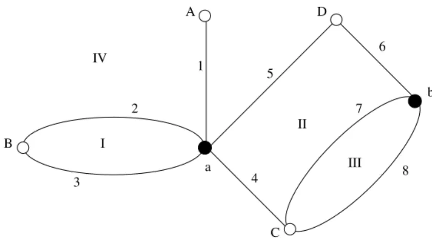
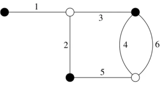
Example 1.2.1. Consider the Dessin in Figure 1.1.

6

8 7

III II

5 A

C 4 a

IV 1

2

3

D

I B

b

Figure 1.1.: Dessin on the plane

The Dessin consists of 8 edges. Hence, the permutations will be inS8. At first, we will deal with the black vertices. In the vertexa five edges meet. If we count them according to the standard positive orientation we get the cycle(12345). For the second black vertex, the vertexb, we get (678). To obtain the permutation we have to combine both cycles.

Now, look at the white vertices. The vertexA is incident with only one edge, the edge 1. Thus, we would get a cycle consisting of only one element, this corresponds to a fixed point in the permutation for the white vertices. The other white vertices give longer cycles. We get(23), (487) and (56) for B,C and D, respectively.

(19)

1.2. About the proof of the Belyi correspondences To assign only one permutation to one kind of vertices we compose the cycles. Since the graph is bipartite, the composition is independent of the order of the cycles. Thereby, we get the permutations σ₀ and σ₁. The last permutation σ∞ can be calculated with help of the first two.

The resulting Belyi permutations are:

σ₀ = (23)(487)(56) σ₁ = (12345)(678)

σ∞=σ₁⁻¹σ₀⁻¹= (1642)(57)

The 4th step: Given a triple of Belyi permutations (σ₀, σ₁, σ∞) fulfilling the properties from Theorem 1.1.8 (iv). The relationσ0σ1σ∞=idleads tohσ₀, σ1, σ∞i=hσ₀, σ1i=:G.

Hence, there is a canonical morphism

ϕ⁰ :hp, qi −→G p7−→σ₀ q7−→σ₁, where hp, qi is the free group generated by two elements.

Definition 1.2.2. SinceΓ(2) is freely generated by the two matrices γ₀ := _{−2 1}^{1 0} and γ₁ := ¹₂⁻²₋₃

it is isomorphic to hp, qi and we get a surjection

ϕ: Γ(2)−→G (1.2.2.1)

γ₀ 7−→σ₀ γ₁ 7−→σ₁.

Let H ⊂ G be the stabilizer subgroup of an edge. Then we define the group Γ ⊂ Γ(2) that we were searching for via

Γ :=ϕ⁻¹(H). (1.2.2.2)

Steps 2 to 4 describe a kind of "algorithm" how to find a subgroup when a Belyi pair is given. Not every step in this "algorithm" has been determined uniquely. Namely, the edges have been numbered randomly and in the end a stabilizer subgroup has been chosen. How does the resulting group Γ vary by doing other choices?

Remark 1.2.3. The construction of the subgroup shows that a different numbering of the edges does not change the group Γ at all; as long as we take the stabilizer to the same edge (the same edge of the Dessin, not the edge with the same number). The numbers are only mean to describe the set of edges.

(20)

Lemma 1.2.4. In the situation of Definition 1.2.2: The choice of another stabilizer subgroup yields a groupΓ⁰ that is conjugated inΓ(2) to the original group Γ.

Proof: LetH = Stab_G(a) and H⁰ = Stab_G(b) be two stabilizer subgroups of G, where a and b represent edges. They correspond to Γ and Γ⁰, respectively. Since G acts transitively, the groups H and H⁰ are conjugated in G. Denote by σ ∈ G an element withσ⁻¹Hσ=H⁰. Fix a matrixγ ∈Γ(2) with ϕ(γ) =σ.

Thenγ⁻¹Γγ = Γ⁰:

Remark that σ(b) =a. Now, take τ ∈ Γ, this element satisfies ϕ(τ)(a) = a. When we conjugate it withγ and map the resulting element toG, we have

ϕ(γ⁻¹τ γ)(b) =σ⁻¹ϕ(τ)σ(b) =b.

Henceγ⁻¹τ γ ∈Γ⁰ and γ⁻¹Γγ ⊂Γ⁰. The other inclusion follows similarly.

Remark 1.2.5. From Lemma 1.2.4 we can see, that a subgroup Γ⊂Γ(2) is uniquely determined by giving a Dessin with an edge that shall be stabilized.

Therefore, in this thesis, to work with a particular subgroup, we will often assume that a Dessin together with a marked edge is given.

The 5th step The subgroup of Γ(2) defined by this procedure in the steps one to four is indeed closely related to the algebraic curve. To understand this relation, we have to introduce some facts.

Lemma 1.2.6. We denote by H = {z∈C|Im(z)>0} the upper half plane, then the group Γ(1) acts on Hvia fractional linear transformation

a b c d

(z) = az+b

cz+d for ^{a b}_{c d}∈Γ(1) andz∈H.

We can add a boundary to H by joining the upper half plane with P¹(Q) ∼=Q∪ ∞, the rational projective line, and getH:=H∪P¹(Q).The action ofΓ(1)onHcan be extended toH by

a b c d

((p:q)) = (ap+bq :cp+dq) for (p:q)∈P¹(Q).

Proof: See [Miy06].

Proposition 1.2.7. LetΓ⊂Γ(1)be a finite index subgroup. The quotientY(Γ) := Γ\H admits the structure of a Riemann surface. The surface Y(Γ) can be compactified with respect to the action on Hto X(Γ) :=Y(Γ).

Proof: See [Shi71].

Remark 1.2.8. Let C be a non-singular algebraic curve defined over a number field.

The group Γ⊂Γ(2) defined via the steps 2,3,4 explained above has the property C(C)∼=X(Γ).

(21)

1.3. The action of the Belyi permutations on a Dessin

We would like to understand better how to imagine the action of the permutationsσ₀, σ₁ and σ∞ in the Dessin.

Since the subgroup of Γ(2) associated to a Dessin is given by the preimage of a stabilizer subgroup, see Equation (1.2.2.2), it is enough to concentrate on the action on a single edge, without loss of generality we may give this edge the number 1.

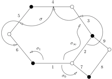
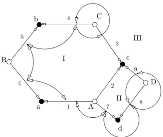
The permutation σ₀ maps an edge to the next edge (according to the orientation) that is incident with the same white vertex, σ1 maps the edge to the next edge that is incident with the same black vertex andσ∞ is, because ofσ∞=σ₁⁻¹σ₀⁻¹, the map that maps an edge not to the next but to the second edge that borders the same cell. The permutations are drawn in Figure 1.2 as arrows. There we have σ0(1) = 7, σ1(1) = 6 and σ∞(1) =σ₁⁻¹σ⁻¹₀ (1) =σ⁻¹₁ (2) = 3.

σ0

σ_∞ 4

σ1

1

2 3 5

6

8 7

9

σ

Figure 1.2.: Action of the permutations σ₀,σ₁ and σ∞

Underϕ, in Formula (1.2.2.1), we were looking at the image of aγ ∈Γ inG=hσ₀, σ₁i.

For the action of the permutations and movements in the Dessin it helps to stay on the level of words in σ0 and σ1. The action of every word inσ0, σ1 and σ∞ on an edge can be visualized as a kind of path in the Dessin. Since we consider the action on edges, the correct graph to find this path in is the corresponding line graph, i.e. the graph where the edges become vertices and that has edges in between two such vertices if the original edges have been adjacent. For our purpose, an intuitive description is sufficient. Let us consider the permutation σ=σ₀σ₁⁻¹σ₀⁻¹σ₁². Its action on the edge 2 is

σ(2) =σ₀σ₁⁻¹σ₀⁻¹σ₁²(2) =σ₀σ₁⁻¹σ₀⁻¹(3) =σ₀σ₁⁻¹(4) =σ₀(5) = 6.

In Figure 1.2, we can see the action of σ on the edge 2 in the Dessin. It determines a sequence of edges in the Dessin: (2,3,4,5,6).

(22)

Remark 1.3.1. LetDbe a Dessin with permutationsσ₀, σ₁and a distinguished edgee.

Then we can imagine elements of Γ(2) as paths in the Dessin and switch between the sets

Γ(2) ←→ {words inσ₀, σ₁} ←→

( paths of adjacent edges in the Dessin starting in e

)

The first arrow is given by replacingγ₀ and γ₁ in a word description of aγ ∈Γ(2) by σ₀ and σ₁, respectively.

The second arrow shall not be understood as a well defined map. There is no way to establish a 1-1 correspondence there. We will go from the set on the left to the set on the right and back. But never in a unique way.

To go from words to paths we will stay on the level of understanding that the path forσ in Figure 1.2 gave.

For the direction from paths to word there is a construction. Let (e₀, e₁, . . . , e_n) be path of edge in a Dessin, i.e. a sequence of edges, whereej andej+1 are adjacent (for all j= 0,1, . . . , n−1). Then we can construct a (not unique) word inσ0 and σ1, therefore inγ₀ and γ₁, out of it: The aim is to get ^Pⁿ_j=1κ_j, where the κ_j are powers of σ₀ and σ1.

Because of the fact thatej and ej+1 (for j∈ {0,1, . . . , n−1}) are adjacent, there exists a vertexV connecting them. Leti_j = 0 if V is white and i_j = 1 ifV is black. There is a powerrj ∈Zwith σ_i^r_j^j(ej) =ej+1. The permutationκn−j :=σ_i^r_j^j will be in the word.

Now, we will discuss the role of the third permutationσ∞:

In the permutations σ₀ and σ₁ there is one cycle for every vertex consisting of the edges that are incident with that vertex. In σ₀ are the cycles for the white vertices, in σ1 the ones for the black vertices. The permutationσ∞plays the corresponding role for the cells. For each cell we find a cycle in σ∞ consisting of edges that border that cell.

Here, it is not possible that all edges for one cell occur, since each edge has two sides and may border two cells. Thus, in average only every second edge occur in the cycle associated to a cell.

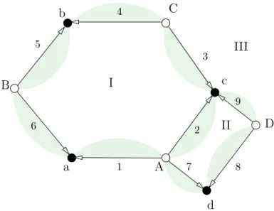
Example 1.3.2. Go back to Example 1.2.1 on page 10. There we have four cells (do not forget the outer cell, the Dessin has to be regarded on the sphere). The cellI corresponds to the fixed point3, the cell II to the cycle(57), the cell III to the fixed point8 and the cellIV to the cycle(1642).

In general: Fix an edge. We can determine for which cell it will be in the corresponding cycle. If we give the edges a direction, see them as directed edges from the white vertex to the black one, then all the edges that contribute to the cycle border the cell with the same side. Taken the standard orientation of the plane, it is the right hand side.

This principle is illustrated in Figure 1.3. From this description one realizes, that every second bordering edge occurs in the cycle.

Now, it is easy so resolve the unsatisfactory fact that, so far, we could determine σ∞

only with help ofσ₀ andσ₁. Let us read offσ∞directly. For a cell choose an edge in the

(23)

1.3. The action of the Belyi permutations on a Dessin

I

III

II D

c b C

B

a A

d

4

1

2 3 5

6

8 7

9

Figure 1.3.: Edges counting for cells

boundary with the property that by turning the edge around its black vertex according to the orientation it is turned into the cell (we will call it property (A)). Starting from such an edge, we count every second edge in the boundary of the cell according to the chosen orientation from the point of view of the center of the cell to get the cycle for that cell. (Note: If there is a vertex with only one edge incident with it, like the edge number 1 in Figure 1.1, both sides of this edge will border the same cell; and both its sides have to be considered.)

The permutationσ∞ is the product of all such cycles for the cells. Since every second edge bordering a cell has the property (A) and every edge has this property regarding to exactly one cell, the cycles are disjoint and their product unique.

How to see that this is the right permutation?

For each Dessin there are two permutations counting every second edge for cells. The one that has just been described and one, where all edges counts for a cell if they fulfill a property (B), that is that by turning the edge around its white vertex it is turned into the cell. For Figure 1.2 or 1.3 this two permutations are

(123)(28)(4976) with property (A) (1538)(246)(79) with property (B).

By the description of the action ofσ∞in Figure 1.2 we can see that the requestσ₀σ₁σ∞= idis only true for the one with property (A). The permutation with property (B) fulfills the identity σ∞σ₁σ₀=id.

Definition 1.3.3. Given a Dessin. We will call an edgee incident with a cell, ife has the property that by turning the edge around its black vertex according to the orientation it is turned into the cell (property (A)).

(24)

For the mapϕ(Equation (1.2.2.1)) that maps Γ(2) into a permutation groupG generated byσ0 and σ1 we have ϕ(γ⁻¹₁ γ⁻¹₀ ) =σ⁻¹₁ σ⁻¹₀ =σ∞. This preimage of σ∞ is

γ_∞:=^{−3 2}_{−2 1}(^{1 0}_{2 1}) = (^{1 2}_{0 1}).

Similar to G that is generated by two permutation out of {σ₀, σ₁, σ∞}, the group Γ(2) is (freely) generated by two matrices out of{γ₀,γ₁,γ_∞}.

Remark 1.3.4. We can interpret the Belyi permutations geometrically. A fundamental domainF_Γfor a subgroup Γ⊂Γ(2) is glued together by [Γ(2) : Γ] fundamental domains F_Γ(2) of Γ(2). The Belyi permutation describe how the generators γ₀,γ₁ and γ_∞ act onF_Γ. Another way of seeing this is: It is encrypted in the Belyi permutations how the F_Γ(2) are glued together to getF_Γ; the permutation σ_i shows the order of gluing at the cuspi(i∈ {0,1,∞}).

1.4. Details on the map between cusps and ramification points

From the construction of Dessins out of Belyi pairs, as explained in Section 1.1 follows that there is a correspondence between branch points of the Belyi pair and the vertices and cells of the Dessin. Beside that, for the subgroup Γ of Γ(2) the so called cusps are related to the vertices and cells of the Dessin. Content of this section is to examine the connection in detail and give an explicit description of the map between the different kinds of cusps.

Definition 1.4.1. Let Γ ⊂Γ(1). The classes of P¹(Q) with respect to the action of Γ are called cusps ofΓ. We will use the word cusp for a representative of a cusp as well.

Lemma 1.4.2. The groupΓ(2) has three cusps of width 2. They are:

n(p:q)∈P¹(Q)|(p, q) = 1,(p, q)≡(0,1) mod 2^o

n(p:q)∈P¹(Q)|(p, q) = 1,(p, q)≡(1,1) mod 2^o (1.4.2.1) n(p:q)∈P¹(Q)|(p, q) = 1,(p, q)≡(1,0) mod 2^o,

thus a system of representatives is {0,1,∞}. The stabilizer of the three cusps are gen- erated by the matrices

γ₀ = _{−2 1}^{1 0}, γ₁=¹₂⁻²₋₃, γ_∞= (^{1 2}_{0 1}). (1.4.2.2) Proof: These are well known facts that are easy to calculate.

Remark 1.4.3. The group Γ(1) has only one cusp, i.e. for all S_j, S_k∈P¹(Q) we find a matrixγkj ∈Γ(1) with γkj(Sj) =Sk, in particular, there is γj ∈Γ(1) with γj(∞) =Sj. Similarly, forSj ∈P¹(Q) we always find a matrix γji ∈Γ(2) such thatγji(i) =Sj where i∈ {0,1,∞}is uniquely determined.

(25)

1.4. Details on the map between cusps and ramification points Definition 1.4.4. Let Γ ⊂Γ(1) be of finite index, S_j ∈P¹(Q) and Γ_j := Stab_Γ(S_j) its stabilizer in Γ. Take γj ∈Γ(1) with γj(∞) =Sj, then

γ_j⁻¹Γ_jγj =ⁿ¹^mb^j

0 1

m∈Z^o,

where bj ∈N and we call bj the width of the cusp Sj (it is easy to check that the width is well defined).

In the following, we will discuss the connection between cusps of the subgroup Γ ⊂ Γ(2), the ramification points of the Belyi pair and the vertices and faces of the Dessin.

Theorem 1.1.8 implies a correspondence between them: For every cusp of a subgroup Γ⊂Γ(2) of width b there exists a vertex or face of the corresponding Dessin of valency

b

2. (We get the factor ¹₂ since for Dessins the base group is Γ(2) where all cusps have width 2.)

But how to find the concrete counterpart?

We will start by illustrating a possibility on an example. Based on the observations there, we will prove the general method.

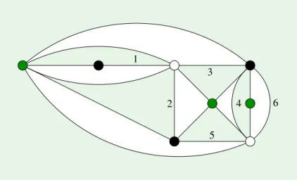
Example 1.4.5. Consider again the DessinDin Figure 1.3 on page 15. We will stabilize edge 1 and get a subgroup Γ⊂Γ(2).

With help of the program in the appendix of [Pos07] we can check that Table 1.1 gives non-equivalent cusps with widths.

Cusp 0 1 2 3 4 5 −¹₂ ¹₂ ¹₃ ²₅ ∞

Width 6 4 4 4 4 6 4 8 4 4 6

Table 1.1.: Cusps and widths for Γ We would like to find the cusps in the Dessin.

The trick is to consider the stabilizer of the cusps and use Remark 1.3.1 to see the stabilizer in the Dessin. Every cusp S_j of Γ has a stabilizer generated by one matrix η_j. We can decompose the generator

η_j =γ_ij⁻¹γ^b_i^j^/2γ_ij,

where bj is the cusp width of Sj, γij ∈ Γ(2) with γij(Sj) = Si a matrix that maps Sj

to S_i ∈ {0,1,∞} and γ_i the generator of Stab_Γ(2)(i) as given in (1.4.2.2). Section 1.3 tells us how to find a path on the edges of the graph D, when we decompose the stabilizer further into its word in γ₀ and γ₁.

The generators of the stabilizers forS_j = 4 and S_l= ²₅ (the most complicated ones in this sample) are

η_j = (γ₁γ₀γ₁)⁻¹γ²₀γ₁γ₀γ₁, η_l= (γ₁γ₀)⁻¹γ²₀γ₁γ₀.

The paths that they describe in the Dessin are sketched in Figure 1.4. We may interpret the movement of η_j as going to an edge incident to C, walking once around C and

(26)

I

III

D c

b C

B

a A

d II

4

1

2 3 5

6

7

9

8

Figure 1.4.: Dessin with stabilizing permutations

going back. A general element of StabΓ(Sj) is (γ₁γ₀γ₁)⁻¹(γ²₀)ⁿγ₁γ₀γ₁ with n∈Z. Its movement is going to an edge incident to C, walking n times around C and going back (ifn is negative, this shall be read as going |n|times backwards around C).

Therefore, is seems to be reasonable to say that C corresponds to the cusp4. Accord- ingly, D corresponds to ²₅.

When we decompose all stabilizer for cusps in Table 1.1 and follow the movements that they imply, we get the results from Table 1.2.

Cusp of Γ Stabilizer Cusp of D

0 γ³₀ A

1 γ²₁ a

2 γ⁻¹₁ γ²₀γ₁ B

3 (γ₀γ₁)⁻¹γ²₁γ₀γ₁ b 4 (γ₁γ₀γ₁)⁻¹γ²₀γ₁γ₀γ₁ C 5 (γ₀γ₁)⁻²γ²₁(γ₀γ₁)² c

−¹₂ γ₀γ²_∞γ⁻¹₀ II

1

2 γ⁻¹₀ γ⁴_∞γ₀ III

1

3 γ⁻¹₀ γ²₁γ₀ d

2

5 (γ₁γ₀)⁻¹γ²₀γ₁γ₀ D

∞ γ³_∞ I

Table 1.2.: Cuss of the subgroup inD

In the Example 1.4.5, we had 11 vertices and faces of the Dessin, we started with 11 non-equivalent cusps of the subgroup and could, by decomposing the stabilizers, assign to each vertex or face exactly one cusp. We will show that that was no coincidence, it

(27)

1.4. Details on the map between cusps and ramification points works in general and the assignment is independent of the representative of the cusp and the choice of the generating element of the stabilizer.

Theorem 1.4.6. LetDbe a Dessin with distinguished edgeeandΓ⊂Γ(2)the subgroup defined by stabilizing e. Then there is a bijection

ν :{cusps of Γ} −→ {vertices and cells ofD} (1.4.6.1) given via

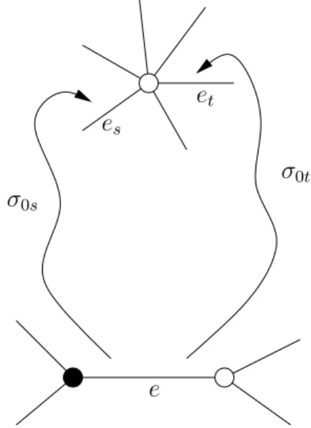
ν(S) :=











the white vertex incident with σ_0s(e) if S ∼

Γ(2) 0 the black vertex incident with σ1s(e) if S ∼_Γ(2) 1 the cell incident withσ∞s(e) if S ∼_Γ(2) ∞

(1.4.6.2)

where s∈S and σis (i∈ {0,1,∞}) is constructed as follows: Let i∼_Γ(2) s be the cusp of Γ(2) to which S is equivalent and γ_is⁻¹γ^b_i^s^/2γ_is be a generating element for Stab_Γ(s), i.e. γ_i is one of the generators

γ₀ =^{−1 0}₂ ₋₁, γ₁ =^{−1 2}_{−2 3} and γ_∞= (^{1 2}_{0 1}), the matrix γ_is ∈Γ(2) with γ_is(s) =iand b_s the width of S.

Then

σ_is :=ϕ(γ_is),

where ϕ : Γ(2) → hσ₀, σ₁i is the map from Formula (1.2.2.1) that maps the generators of Γ(2) to the permutations associated toD.

Before we come to the proof, we make the following

Remark 1.4.7. In Equation (1.4.6.2), the image under ν of a cusp S of γ ⊂ Γ(2) is defined via a representative s∈S, therefore, by abuse of notation, we will useν for the underlying map of the rationals as well:

ν :Q∪ ∞ −→ {vertices and cells ofD}

Proof: To prove the Theorem 1.4.6, we will show the following properties:

(i) The mapν is well defined on the level of rational number, i.e. fors∈Qthe matrix γ_is exists and the image is independent of the particular choice.

(ii) The map ν is well defined on the level of cusps, i.e. independent of the choice of the representative in a cusp.

(iii) The mapν is injective.

(iv) The mapν is surjective.