Dissertation
submitted to the
Combined Faculties for the Natural Sciences and for Mathematics of the Ruperto–Carola University of Heidelberg, Germany
for the degree of Doctor of Natural Sciences
presented by
Diplom–Physiker Claus Zahlten born in Heidelberg
Oral examination: February 11, 2004
B¨ odeker’s Effective Theory:
From Langevin Dynamics to Dyson–Schwinger Equations
Referees: Prof. Dr. Michael G. Schmidt Prof. Dr. Klaus-Dieter Rothe
Dyson–Schwinger–Gleichungen f¨ ur die Langevin–Dynamik in B¨ odekers effektiver Theorie
Zusammenfassung
Trotz schwacher Kopplung wird in nicht-abelschen Eichtheorien bei hoher Temperatur die Dynamik der Felder nicht-perturbativ, wenn die beteiligten Impulse von der Gr¨oßenordnung
|k| ∼g2T sind. Solche Verh¨altnisse sind typisch f¨ur die Prozesse der elektroschwachen Verletzung der Baryonenzahl im fr¨uhen Universum. B¨odeker gelang die Ableitung einer effektiven Theorie, die die Dynamik der Feldmoden mit kleinen Impulsen durch eineLangevin–Gleichung beschreibt.
Diese effektive Theorie wurde bislang f¨ur Gitterrechnungen verwendet. In der vorliegenden Arbeit stellen wir einen komplement¨aren, analytischeren Zugang ¨uberDyson–Schwinger–Gleichungen vor. B¨odekersLangevin–Gleichung wird hierzu mithilfe von Methoden, die aus der stochasti- schen Quantisierung bekannt sind, in ein Pfadintegral umgeschrieben. Wir argumentieren, daß die sp¨atere Trunkierung derDyson–Schwinger–Gleichungen die Einf¨uhrung von Eichgeistern notwendig macht, die in stochastischer Quantisierung normalerweise nicht auftreten. Dies f¨uhrt auf eine BRST symmetrische Formulierung und zugeh¨origeWard–Takahashi–Identit¨aten. Eine zweite BRST Symmetrie, die den Ursprung der Theorie in einer stochastischen Differential- gleichung widerspiegelt, wird durch die Einf¨uhrung der Eichgeister zerst¨ort. Dennoch lassen sich die zugeh¨origen (stochastischen) Ward–Identit¨aten aus der fundamentalen Struktur der The- orie ableiten und bewirken eine K¨urzung verschiedener Terme der Eich–Ward–Identit¨at. Zur Kl¨arung einiger spezieller Fragen leiten wir die Feynman–Regeln der Theorie ab und f¨uhren einige perturbative Rechnungen aus. Schließlich leiten wir dieDyson–Schwinger–Gleichungen ab und schlagen eine m¨ogliche Trunkierung vor, die zumindest approximativ die stochastischen und Eich–Ward–Identit¨aten respektiert.
B¨ odeker’s Effective Theory: From Langevin Dynamics to Dyson–Schwinger Equations
Abstract
The dynamics of weakly coupled, non-abelian gauge fields at high temperature is non-perturbative if the characteristic momentum scale is of order|k| ∼g2T. Such a situation is typical for the processes of electroweak baryon number violation in the early Universe. B¨odeker has derived an effective theory that describes the dynamics of the soft field modes by means of aLangevin equation. This effective theory has been used for lattice calculations so far. In this work we provide a complementary, more analytic approach based onDyson–Schwingerequations. Using methods known from stochastic quantisation, we recast B¨odeker’s Langevin equation in the form of a field theoretic path integral. We argue that a physically reasonable truncation of the Dyson–Schwinger equations requires the introduction of gauge ghosts, which in general is not mandatory in stochastic quantisation. This leads to a BRST symmetric formulation and to correspondingWard–Takahashiidentities. A second BRST symmetry reflecting the origin in a stochastic differential equation has to be sacrificed to establish the gauge BRST symmetry. The (stochastic) Ward identities can still be obtained by referring to the underlying structure and are shown to produce a cancellation among several terms of the gauge Ward identity. To clarify some issues, we derive theFeynman rules and perform some perturbative calculations. Finally, we deduce theDyson–Schwingerequations and suggest a truncation scheme that approximately respects the gauge and stochastic Ward identities.
“Orba parente suo quicumque volumina tangis, his saltem vestra detur in urbe locus.
quoque magis faveas, non haec sunt edita ab ipso, sed quasi de domini funere rapta sui.
quicquid in his igitur vitii rude carmen habebit, emendaturus, si licuisset, eram.”
[Ovid, Tristia]
Contents
1 Introduction 3
2 Baryon Number Violation and B¨odeker’s Effective Theory 10
2.1 Baryon Number Violation in SU(2) Gauge Theory . . . 10
2.2 B¨odeker’s Effective Theory . . . 11
3 Path Integral Formulation of B¨odeker’s Theory 17 3.1 From Stochastic Differential Equations to Path Integrals . . . 18
3.2 B¨odeker’s Theory: Upgrading toκGauge . . . 23
3.3 The Path Integral Formulation . . . 28
4 BRST Symmetric Action and Ward–Takahashi Identities 31 4.1 Constructing a BRST Symmetric Action . . . 33
4.2 Symmetries of the Theory and their Implications . . . 37
4.2.1 Gauge Ward Identities . . . 37
4.2.2 Stochastic Ward Identities . . . 39
4.2.3 Translational and Rotational Invariance . . . 47
4.2.4 Ghost Number Conservation . . . 49
4.3 Explicit Consequences to Lower N-Point Functions . . . 51
4.3.1 Definitions and General Relations . . . 51
4.3.2 Simple Consequences of Translational and Rotational Invariance . . . 54
4.3.3 The Gauge and Stochastic Ward Identities . . . 56
5 Perturbation Theory 62 5.1 Feynman rules . . . 62
5.1.1 The Propagators . . . 62
5.1.2 The Vertices . . . 69
5.2 UV Behaviour and Cancellations . . . 73
6 Dyson–Schwinger Equations 78 6.1 General Dyson–Schwinger Equations . . . 78
6.1.1 Anti-ghost (¯ω) equation . . . 78
6.1.2 Ghost (ω) equation . . . 80
6.1.3 Auxiliary field (λ) equation . . . 80
6.1.4 Gauge field (A) equation . . . 81
6.2 Explicit Equations for Lower N-Point Functions . . . 82
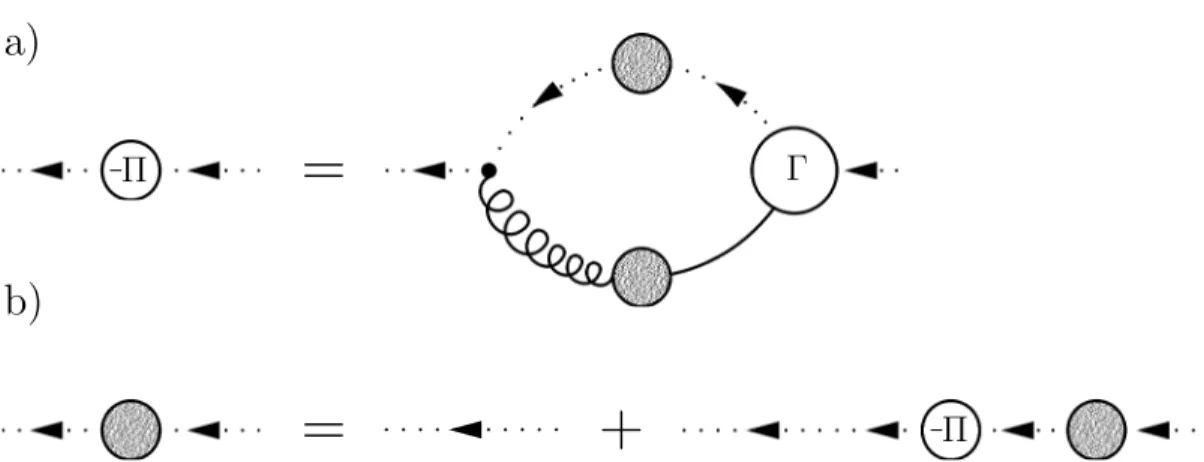
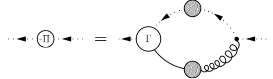
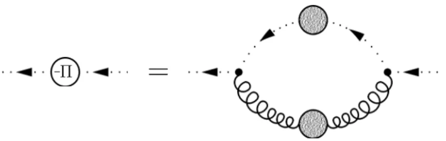
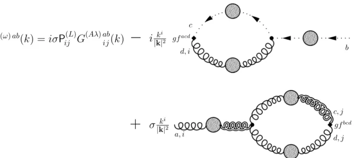
6.2.1 DSE for Π(ω) . . . 83
6.2.2 DSE for Π(λλ) . . . 86
6.2.3 DSE for Π(λA) . . . 88
6.2.4 DSE for Π(Aλ) . . . 89
6.2.5 DSE for Π(AA) . . . 91
7 Conclusions and Outlook 93
1
A Conventions and Useful Relations 98
B Feynman Rules 102
Bibliography 104
Chapter 1
Introduction
Despite the fact that philosophy has not come to a definite conclusion on the issue yet, for the rest of the world it is one of the best and best proven features of the Universe that it really exists. However, if we ask ourselves whether we understand why it exists, we have to become fairly modest or even muttering a fainttacuissemus.
For more than seventy years now, we have known of the existence of antimatter. Since Dirac postulated the anti-electron or positron in 1928, which was discovered in cosmic rays by Anderson four years later, it became clear that in fact to any species of elementary particles in nature there exists a corresponding anti-particle. Any particle and its anti-particle differ in having opposite inner quantum numbers like, e.g., the electric charge, but are identical with respect to their other properties like masses, spin etc. Besides the difference caused by their opposite charges, particles and anti-particles behave in almost the same way, i.e. the fundamental laws of nature only slightly distinguish between matter and antimatter (in fact, only the weak interactions show any distinction at all). Furthermore, on this fundamental level, nature does not favour matter over antimatter in any respect: After decades of research at the large accelerator laboratories with millions of tracked particle reactions it wasnever observed that any particle had been created without the corresponding anti-particle.
In sharp contrast to this symmetry on the microscopic level is our everyday experience that the macroscopic world seems to consist exclusively of matter. Moreover, coming back to our question at the beginning, if equal amounts of matter and antimatter have been created at the big-bang and if the laws of physics are essentially symmetric between matter and antimatter, why is there anything left at all? A complete annihilation of the matter and antimatter contents of the Universe should be expected, leaving nothing to say but “. . . and the rest wasγ–rays”.
It is therefore a fascinating challenge for modern physics to find an explanation of this startling discrepancy between the observed balance of matter and antimatter on the microscopic level and the predominance of matter in the macroscopic world.
Is there really no antimatter?
The first question that naturally arises is, of course, whether this discrepancy persists in view of a more careful investigation: Is there really no antimatter in the Universe and how do we know this? First of all, we know by direct experience that our own planet entirely consists of matter. The same can be inferred for the sun and the other celestial bodies in the solar system from the composition of the solar wind and the rather frequent hits the planets suffer by straying meteorites.
However, as we have mentioned above, there is indeed a certain amount of antimatter observed in the cosmic rays. These consist mainly of energetic protons andαparticles and contain at a ratio of 10−4 also anti-protons. This fraction of anti-protons, however, is consistent with a secondary production by interactions of the energetic protons with the interstellar medium according to the processp+p→3p+ ¯p.
3
The observed lack of a considerable admixture of an antimatter component to the cosmic rays exceeding the level that is expected from secondary processes and especially the complete absence of anti-nuclei in cosmic rays therefore indicate that no significant amounts of antimatter exist within our galaxy.
Furthermore, the space between galaxies in clusters is not empty. It contains non-negligible amounts of gas as revealed by x–ray emissions. If clusters contained matter and antimatter galaxies at the same time, this would lead to strong annihilation signals with the intergalactic gas. Those signals are not observed leading to the conclusion that there is no coexistence of matter and antimatter within domains up to the typical size of galactic clusters [1].
At first sight, this leaves the possibility of a matter–antimatter symmetric Universe where regions dominated by matter or antimatter are typically larger than 20 Mpc and separated by extensive voids. However, apart from the open question by which mechanism such a separation could be produced, Cohen, De R´ujula and Glashow have shown in a detailed analysis [2] that such a scenario is incompatible with present observations: The uniformity of the cosmic microwave background (CMB) sets an upper limit to the inhomogeneities in the matter distribution at the time of last scattering. Thereby it restricts the maximal size of possible voids at this stage. Cohen et al. argue that this maximal size is too small to prevent them from being destroyed by diffusion processes and that direct contact between matter and antimatter domains would therefore be unavoidable, at least during the epoch from last scattering to the onset of structure formation.
The annihilation photons from the contact zones would contribute to the cosmic diffuseγ–ray spectrum (CDG). This is clearly excluded by experiment. Independently, relativistic electrons from the annihilations should lead to a distortion of the CMB spectrum, directly by Compton scattering and indirectly by heating the medium. However, present measurements of the CMB spectrum are not restrictive enough to provide a reliable test via this second effect.
Altogether we conclude that observational evidence is quite strong that the Universe did not contain considerable amounts of antimatter back to the times of last scattering.
Ex nihilo nihil fit — or, maybe it does . . .
The matter/antimatter asymmetry of the Universe can be quantified by the difference of the number densities of baryons and anti-baryons. Because the latter is essentially zero today, it is given by the present density of baryons, which in turn is quite accurately known today. There exist two independent methods for its determination, which lead to consistent results: nucleosynthesis and CMB anisotropies.
The well understood mechanism of nucleosynthesis tightly links the primordial abundances of the light elements D, 3He, 4He and 7Li to the baryon density nB. Measurements of these abundances can therefore be used to determinenB. The four element abundances have different functional dependences on the baryon density and it is therefore a nontrivial result that all of them consistently lead to a baryon density (that is conventionally normalised to the photon density) of (see Ref. [3])
2.6·10−10≤ nB
nγ ≤6.2·10−10
From a systematical point of view, deuterium measurements yield the most convincing results because the abundance is not affected by astrophysical processes and thus one directly measures the primordial value. In the other cases systematical errors can be minimised by restricting to regions of low metallicity indicating negligible star activity.
An independent way of determining the baryon density has opened up since precision measure- ments of the CMB spectrum are available. Acoustic oscillations of the coupled photon–baryon plasma during recombination leave an imprint on the CMB spectrum that is sensitive to nB. Though this method relies on certain theoretical assumptions on the nature of primordial density fluctuations (see Ref. [4] for a discussion), it is still remarkable that the value inferred from CMB anisotropies is consistent with the nucleosynthesis bounds above.
Summarising this observational evidence, we can state that we know the baryon density and therefore the baryon asymmetry of the Universe quite well by now. The question to be posed is
5
whether we can understand this value in terms of fundamental physics.
Though an ad hoc explanation by initial conditions seems to be possible at first, this is not really true on looking more carefully. Two major arguments disfavour this possibility: If the evolution of the Universe underwent an inflationary period (which becomes more and more plausible), inflation would dilute away any difference in the baryon and anti-baryon densities leaving behind a baryon symmetric Universe. In addition to that, as we will see below the Standard Model itself (that is the part of physics we know tobe realised in nature independent of all possible extensions thatmay be realised) leads to efficient baryon number violating processes in the early Universe at temperatures where the electroweak symmetry is still unbroken. These processes inevitably destroy any prior existing baryon asymmetry, at least if not based on a non-vanishing difference between baryon and lepton number, which is exactly conserved in the Standard Model.
Consequently, it is rather likely that at some point during the evolution of the Universe its baryon asymmetry was zero and the puzzle persists how the present asymmetry could evolve.
In 1967 Sakharov identified three necessary conditions for a dynamical generation of a baryon asymmetry to be possible [5]
• B violation
• C and CP violation
• departure from thermal equilibrium
Besides B violation, which is obvious, C and CP violation are necessary to allow for a difference in the reaction rates for processes generating particles and such generating anti-particles. In thermal equilibrium the number densities of particles and anti-particles had to be equal according to their equal masses.
In search of a situation in the history of the Universe where Sakharov’s criteria could have been fulfilled, two major scenarios appear natural: The necessary departure from thermal equilibrium could have been provided by an out–of–equilibrium decay of a heavy particle or alternatively by one of the phase transitions assumed to have taken place.
Scenarios of the first kind are typically considered in the context of Grand Unified Theories.
These offer at the same time the possibility of new B, C, and CP violating interactions as well as a variety of candidates for the decaying particle. This freedom, on the other hand, may be rated as a weakness of these models, especially in view of the fact that the GUT scale physics involved is far out of the reach of experiment.
Baryon number generation via a phase transition in the early Universe seemed especially promising when it became clear that in principle the Standard Model itself contains all of the ingredients that are necessary for such a scenario. Today, it is known that these models do not work in the strict version of the Standard Model. However, within certain extensions like the Minimal Supersymmetric Standard Model (MSSM) or the Next-To-Minimal Supersymmetric Standard Model (NMSSM) they seem quite possible [6–17]. These supersymmetric extensions, on the other hand, are well motivated by a number of independent considerations and, in contrast to the GUT physics, they are maybe “just around the corner” of present-day experiments.
The general scenario is the following: Departure from thermal equilibrium is provided by the electroweak phase transition. C and CP violation are clearly present within the Standard Model.
Thus, the most interesting question is the one of B violation.
As we have pointed out above, there has never been the slightest evidence for B violation in any of the high energy physics experiments that are so well described by the Standard Model.
Nevertheless, it was found by ’t Hooft [18] that baryon number in the Standard Model is indeed violated due to theBell–Jackiw anomaly [19, 20] and the non-trivial structure of the SU(2) vacuum.
The vacuum configurations of the SU(2) gauge field fall into disjoint classes that at zero tem- perature cannot be continuously transformed into each other without leaving the space of vacuum configurations. The individual classes (labelled by a topological invariant, the Chern–Simons
number, and corresponding to a specific baryon number) are therefore separated by an energy barrier. The change in the baryon or Chern–Simons number between two classes is related to the field configuration mediating the transition
B(t2)−B(t1) =nF
£NCS(t2)−NCS(t1)¤
=nF g2 32π2
t2
Z
t1
d4xtrFF˜ (1.1) wherenF is the number of fermion families,gthe weak coupling andF the SU(2) field strength.
At zero temperature, a transition between vacua of different classes (and thus different baryon number) can only proceed by quantum tunneling via instanton field configurations. It was already calculated by ’t Hooft that such processes are typically suppressed by a factor of 10−173 which explains why they have never been observed.
At temperatures of order 100 GeV near the electroweak phase transition, however, transitions over the barrier can occur by classical, thermal fluctuations [21]. These so-called sphaleron transi- tions are suppressed by aBoltzmannfactor only and in principle can become quite efficient [23].
If the temperature exceeds the critical temperature of the electroweak phase transition, even the barrier between different vacua vanishes. The rate of baryon number violating processes in this regime is referred to as “hot sphaleron rate”. A better understanding of this rate and of the physics involved constitute the main motivation of this work.
Let us now describe the assumed mechanism of baryon number generation during the elec- troweak phase transition in extensions of the Standard Model (see, e.g., Ref. [22]). It is essential for the mechanism to work that the phase transition is strongly of first order (which is one of the reasons why it does not work in the strict version of the Standard Model where only a cross-over takes place). The phase transition then proceeds via the nucleation of “bubbles” of the broken phase (with Higgs expectation valuehHi 6= 0) within the still symmetric phase Universe. In the symmetric phase where the Higgs expectation value ishHi= 0 baryon number changing processes are fast. Inside the bubbles, the sphaleron transitions are assumed to be rapidly switched off (we come to this point soon).
During the phase transition, the individual bubbles expand and fuse until they fill the whole Universe and the phase transition is complete. For the particles in the hot plasma a passing bubble wall creates the necessary departure from equilibrium to make baryon number generation possible. By C and CP violating interactions of the particles in the plasma with the bubble wall a difference in the number densities of left-handed particles and their anti-particles is generated in the symmetric phase directly in front of the moving bubble wall. The baryon number changing processes in the symmetric phase translate this difference into a baryon/anti-baryon asymmetry that subsequently is transferred into the bubble. If sphaleron transitions inside are switched off fast enough, the asymmetry is frozen in and persists until today. If not, it would be destroyed again. Likewise, the asymmetry would be washed out if the baryons and anti-baryons would stay too long outside in the symmetric phase.
Obviously, a delicate balance is necessary to create the observed baryon asymmetry by this mechanism: The condition that sphaleron processes inside the bubble are switched off fast enough provides an upper bound on the Higgs mass which for the Standard Model by now is far below the experimental bounds excluding baryon number generation via this mechanism in the strict Standard Model. In addition to that, the produced baryon asymmetry is sensitive to the CP violating process rates at the bubble wall, to the transport in the symmetric phase in front of the wall, to the velocity of the bubble wall itself and finally to the exact rate at which the baryon number changing processes occur in the symmetric phase.
The rate of baryon number violation in the symmetric phase
The field configurations responsible for considerable changes in the baryon number need to have a minimum spacial extent: According to Eq. (1.1), a configuration of sizeR must have a field strength& 1/gR2 to mediate a change in the Chern–Simons number of order one. This corre- sponds to an energy cost&1/g2Rand in order to be unsuppressed therefore requiresR&1/g2T.
7
In fact, because smaller configurations are favoured against larger ones due to entropy, the baryon number changing processes are dominated by field configurations at the lower bound, i.e. processes with the characteristic momentum scaleg2T [23].
However, this is the scale at which finite temperature perturbation theory breaks down in non- abelian gauge theories [24, 25]. The hot sphaleron rate therefore is determined by non-perturbative physics and cannot be calculated by using weak coupling methods.1
The dynamics of the soft modes of the gauge field with spacial momenta|k| ∼g2T is essentially classic [26]. This is a consequence of the large occupation numbers of these modes at the high temperatures in the symmetric phase. For a long time it was thought that the hard modes|k| ∼T decouple and have no influence on the soft dynamics. Consequently, R ∼1/g2T would be the only scale relevant to the problem and by simple dimensional arguments the number of sphaleron transitions per unit time and volume was assumed to have the parametric form Γ∝R−4∝g8T4. However, Arnold, Son and Yaffe found that the hard modes in fact do influence the soft dynamics [27]. As was known before, interactions with the hard modes lead toDebyescreening of the soft (non-abelian) electric fields and therfore only the transverse modes of the soft fields are determining the sphaleron rate. Static magnetic fields are unscreened. However, the field configurations mediating transitions between different Chern-Simons numbers are not completely static. This leads toLandaudamping effects restricting the frequency scale of the soft magnetic modes that are relevant to sphaleron transitions tok0∼g4T rather thang2T as was assumed by comparison with the scale of spacial momenta before. Accordingly, Arnold et al.corrected the estimate for the hot sphaleron rate to Γ∝g10T4.
Because of the influence that hard modes have on the soft dynamics they cannot be simply disregarded in constructing an effective classical theory for the soft modes. However, the hard modes are weakly coupled and can be integrated out in perturbation theory. At leading order this yields the well-known hard thermal loop (HTL) effective theory [28].
B¨odeker realised that the dynamics of the soft modes is still affected by so-called semi-hard modes |k| ∼gT via hard thermal loop induced interactions [29, 30]. This effect is intrinsically non-abelian and has no analogue in abelian gauge theories. In a quasi-particle description of the hard modes, interactions of the hard with semi-hard modes correspond to small-angle scatterings of the former. Small-angle scatterings in abelian gauge theory have hardly an effect on the current that is carried by the particles and ultimately seen by the soft modes. This is completely different in non-abelian gauge theories, where even a small-angle scattering can alter the charge of a particle entirely. The randomisation of the colour charges via these interactions leads to a logarithmic enhancement of the characteristic frequency scalek0 ∼g4ln(1/g)T and thereby to the parametric form Γ∝g10ln(1/g)T4of the hot sphaleron rate.
The semi-hard modes are still perturbative and B¨odeker succeeded in deriving an effective theory for the soft modes alone by integrating out the modes |k| ∼ gT from the hard thermal loop effective theory [29, 30]. At leading order ing one obtainsVlasov–Boltzmannequations with a gaussian noise and a collision term. Besides the soft modes of the gauge field these equations contain the soft fluctuations of the hard particle distribution function.
To leading logarithmic order (LLO) the Boltzmannequation can be solved and one is left with an effective theory that only contains the soft modes of the gauge field (see also Ref. [31]).
This effective theory, that is commonly referred to as ‘B¨odeker’s theory’, has the form of a stochastic differential equation of theLangevin type and shows a much better UV behaviour than the original HTL effective theory. All influence that higher momentum modes have on the soft sector is encoded within a single parameter (the colour conductivity) and a gaussian white noise term.
B¨odeker’s theory was originally derived to serve as basis for a lattice approach to the non- perturbative dynamics of soft non-abelian gauge fields. This program has been pursued in Ref. [32]
where the sphaleron rate was calculated for the case of pure SU(2)Yang–Millstheory. In view of electroweak baryogenesis, one is ultimately interested in the rate at temperatures close to the
1Recall that this doesnotmean that the gauge couplinggis large. It means that the contributions of diagrams with additional loops are no longer small if the momentum is of orderg2T, and therefore cannot be treated as a perturbation.
electroweak phase transition. A prioriit is questionable whether pureYang–Millstheory gives the right answer in that regime. In Ref. [33] the sphaleron rate was therefore recalculated in the presence of a light Higgs degree of freedom. It was found that in case of a phase transition that is strong enough to prevent the baryon asymmetry from wash-out, the influence of the Higgs field is rather moderate (about 20%). It was also argued that the result should hold for the MSSM too.
Lattice calculations are an ideal tool to extract with a minimum of theoretical prejudice a specific piece of information from a given theory. However, in a sense, they are kind of a ‘black box’ that give the answer but hide the wayhow that answer does come about.
The aim of this work is to provide a complementary, more analytic approach to the non- perturbative physics encoded in B¨odeker’s effective theory. The emphasis thereby lays not pri- marily on the accuracy of the results where it is hardly possible to beat the lattice calculations.
Our aim is to provide a tool for a deeper understanding of what is really going on in the non- perturbative sector of hot non-abelian gauge theory and during creation of baryon number.
Such a deeper understanding is not only important for baryogenesis and the determination of the sphaleron rate. Magnetic screening and the corresponding identification of a magnetic mass are of quite general theoretical interest with applications also in the field of heavy ion collisions and the physics of the quark–gluon plasma [34–37].
The key idea of this work is rather simple. B¨odeker’s effective theory has the form of a Langevin equation. It is well-known from stochastic quantisation that a Langevin equation can be recast in the form of a path integral [38–40]. This path integral then can be reinterpreted as the functional integral formulation of an euclidean quantum field theory with some ‘strange’
action. In this way, one gains access to all the powerful methods developed in QFT. Especially, it is possible to derive theDyson–Schwinger equations of the theory offering an approach to the non-perturbative sector that is independent from and complementary to the existing lattice studies.
On the way to this goal a couple of obstacles have to be overcome. These are mostly related to the peculiar role played by gauge invariance in the context of stochastic quantisation and B¨odeker’s effective theory. A thorough understanding of this role proves to be essential in pursuing our aim.
The outline of this work is as follows. In Chapter 2 we briefly describe baryon number violation in SU(2) gauge theory and discuss the derivation of B¨odeker’s effective theory.
Chapter 3 is devoted to the transcription of B¨odeker’s theory in path integral form. We describe the general formalism of translating a stochastic differential equation into a path integral.
The transcription leads to characteristic structure of the action, that can be expressed in form of a BRST symmetry (so-called stochastic BRST symmetry).
This formalism shall be applied to B¨odeker’s theory. However, in the end of the day, one will be forced to rely on a certain truncation scheme to extract any concrete results from the Dyson–Schwingerequations that we are aiming for. This truncation may introduce a possible gauge dependence and thus may render the results worthless. To keep control over the gauge dependence, it is therefore necessary to generalise B¨odeker’s equation from A0 = 0 gauge to a more general class of gauges before applying the formalism.
Gauge fixing in a stochastic differential equation is quite delicate. One has to make sure not to destroy theMarkovian nature of the equation. Applying methods developed in the context of stochastic quantisation [41], we introduce a gauge fixing term into B¨odeker’s equation thereby achieving the desired upgrade to a general class of flow gauges. The application of these methods in the case of B¨odeker’s theory requires some generalisation to cope with the different role of the time variable in stochastic quantisation. The argumentation leading to the introduction of the gauge fixing term will be essential also in the construction of a (gauge) BRST symmetric action in the following chapter.
In Chapter 4 we argue that any physically reasonable truncation of theDyson–Schwinger equations requires the introduction ofgauge ghosts (to be distinguished from the ghosts fields carrying thestochasticBRST symmetry above; we refer to the latter as equation of motion (EOM) ghosts). In the full, untruncated theory gauge ghosts are not necessary, which is generally true in stochastic quantisation [39, 41]. As was shown in Ref. [41], gauge ghostscan be introduced in
9
stochastic quantisation in order to establish a gauge BRST symmetric formulation.
We carry out this program in the case of B¨odeker’s theory and derive theWard–Takahashi identities corresponding to the gauge BRST symmetry of the action. These should be respected by the truncations to be used.
The gauge Ward identities are not the only restrictions to be observed. A second class of Ward identities exist, that are related to the characteristic structure of the theory reflecting its origin in a stochastic differential equation. This characteristic structure is originally expressed by the stochastic BRST symmetry. Introducing the gauge ghosts, however, destroys this symmetry.
Nevertheless, it does not change the physical contents of the theory. The stochastic BRST symmetry is only an elegant way to express this structure. By directly referring to the underlying physics, it is still possible to derive the corresponding stochastic Ward identities. They provide the second building block of restrictions to be imposed on the truncations.
Chapter 5 contains a discussion of the perturbation theory based on the path integral formu- lation of B¨odeker’s effective theory. This allows to understand some of the general results of the preceeding chapters from a different point of view. We derive theFeynmanrules and perform a number of selected perturbative calculations clarifying some questions concerning the elimination of EOM ghosts and the ultraviolet behaviour of the theory.
In Chapter 6 we derive the Dyson–Schwinger equations of B¨odeker’s effective theory. In combination with the gauge and stochastic Ward identities of Chapter 4, this constitutes an independent approach to the non-perturbative dynamics of the soft, non-abelian gauge fields encoded in B¨odeker’s effective theory.
In Chapter 7 we summarise and discuss our results and offer a first suggestion of a truncation scheme to be used in an implementation of our formalism.
Finally note that a summary of the conventions used in this work together with a number of useful relations can be found in Appendix A. For easier reference, a compilation of theFeynman rules derived in Chapter 5 is provided in Appendix B.
Baryon Number Violation and B¨ odeker’s Effective Theory
In this chapter we briefly recall the origin of baryon number violation in the Standard Model for the mere sake of motivation. In addition to that and more importantly, we describe the derivation of B¨odeker’sLangevinequation providing the basis of this work.
2.1 Baryon Number Violation in SU(2) Gauge Theory
Baryon number violation in the Standard Model is due to electroweak physics. Thus, let us have a look at theLagrangedensity of Weinberg–Salamtheory. It reads
L=−1
4Fµνa Faµν−1
4BµνBµν+ (Dµφ)+Dµφ−V(φ) +Lf (2.1) with theSU(2)L field strength
Fµνa =∂µAaν−∂νAaµ−g εabcAbµAcν (2.2) theU(1)Y field strength
Bµν =∂µBν−∂νBµ (2.3)
the covariant derivative
Dµ=∂µ+igAaµτa 2 + i
2g0Bµ (2.4)
theHiggspotential
V(φ) = λ
4(φ+φ−v2)2 (2.5)
and finally (but most importantly to us) the fermionic sector Lf = Ll +Lq. The electron contribution to the fermionic sector, for example, is
Le= ¯ψLiγµDµψL+ ¯eRiγµDµeR−ce(¯eRφ+ψL+ ¯ψLφ eR) (2.6) with identical contributions of the other leptons and analogous (i.e.Cabbiborotated) ones of the quarks. The important observation is now the following: Because the projectors to the left- and right-handed fields containγ5, the fermionic sector contains an axial current ¯ψγµγ5ψ coupled to the SU(2) gauge field. Such a current is known to suffer from a quantum anomaly [19, 20]
∂µjeµ= g2
32π2Fµνa F˜aµν− g02
32π2BµνB˜µν (2.7)
10
2.2. B¨odeker’s Effective Theory 11
with the same expression for the other fermions of the theory. We therefore find for the total leptonic current
∂µjLµ=X
l
∂µjlµ=nF∂µjeµ (2.8)
wherenF is the number of fermion families. For the baryonic current one has
∂µjBµ =X
q
∂µjµq = (nFnC) 1
nC∂µjeµ=nF∂µjeµ (2.9) wherenCis the number of colours, i.e.nFnC the number of different quarks, and 1/nCtakes care of the fact that the lepton number of an electron is one but the baryon number of a quark 1/3.
Altogether we find
∂µ(jBµ−jµL) = 0 (2.10)
∂µ(jBµ+jµL) 6= 0 (2.11)
and thus conclude thatB+Lin the electroweak theory is violated whileB−Lis not. Furthermore, integrating Eq. (2.7) yields (the hypercharge field does not contribute)
∂0
Z
d3x jB0 =nF g2 32π2
Z
d3x Fµνa F˜aµν (2.12) and consequently
B(t2)−B(t1) =nF g2 32π2
t2
Z
t1
d4x Fµνa F˜aµν (2.13) which we had claimed in Eq. (1.1). Whenever the gauge field evolves in such a way thatR
d4xtrFF˜ is non-zero, then the baryon number will change.
The next question is of course, whether such field configurations really exist. As we have explained in the introduction they actually do. At zero temperature, the different vacua are separated by an energy barrier and a transition can occur by quantum tunneling via instanton field configurations (which is highly suppressed). At high temperature, sphaleron transitions become possible: classical transitions over the top of the barrier by thermal fluctuations. At even higher temperatures, finally, the electroweak symmetry is restored and the barrier between different vacua vanishes. The so-called hot sphaleron rate in this regime then is determined by the Chern–Simons number diffusion rate.
2.2 B¨ odeker’s Effective Theory
In this section we give an outline of the derivation leading to B¨odeker’s effective theory. However, a word of caution may be in order. We do not claim to give a self-contained description of B¨odeker’s work. In the course of the derivation, several approximations have to be made. To reallyjustify these approximations requires a much more detailed analysis [29, 30]. Our aim is to explain the main ideas leading B¨odeker to hisLangevinequation and thereby to set the stage for what will be our topic for the rest of this work.
As we have mentioned in the introduction, the starting point of B¨odeker’s derivation is the HTL effective theory. In this effective theory, the hard modes of momenta|k|&T have al- ready been integrated out, i.e. effective propagators and vertices for the field modes with|k| ¿T have been constructed by considering loop diagrams with small external momenta|k| ¿T and loop momenta of orderT.
To proceed and integrate out the semi-hard modes|k|&gT, it would be straightforward to use these HTL effective propagators and vertices and to calculate diagrams with soft external and semi-hard loop momenta. This has been pursued at one-loop level in Ref. [42]. However, the one- loop approximation proves to be insufficient. Going beyond one loop, on the other hand, is quite
a tedious task in the HTL effective theory. Fortunately, an alternative formulation of the HTL effective theory in terms of kinetic equations [43] exists and B¨odeker realised that semi-hard modes can be ‘integrated out’ in kinetic theory.
The kinetic formulation of the HTL theory comprises the gauge field containing the field modes with|k| ¿T and a field Wa(x,v) that describes the deviation of the phase space density of hard particles (modes) from the equilibrium distribution. Thus, the modes with|k| ¿T are described as classical fields (corresponding to their high occupation numbers) and the hard modes as quasi-particles. The vectorvis their three-velocity withv2= 1 andv= (1,v). The dynamics of the system is then described by
[Dµ, Fµν(x)] = m2D Z dΩv
4π vνW(x,v) (2.14)
[v·D, W(x,v)] = v·E(x) (2.15)
The first of these equations is simply the (non-abelian)Maxwell equation for the field modes with|k| ¿T under the influence of a current produced by the hard modes. The second equation in turn is aBoltzmannequation governing the evolution of the hard particle phase space density in the presence of the field modes.
In order to integrate out also the semi-hard modes and to obtain an effective theory for the soft modes alone, that both are contained within the field modes so far, B¨odeker now introduces a separation scaleg2T ¿µ¿gT and a corresponding split of all quantities into theirFourier components with soft spacial momenta|k| < µ and semi-hard ones |k| > µ. It is essential, of course, that finally any dependence on the separation scale drops out. Inserting the decomposition into soft (uppercase) and semi-hard (lowercase) modes
A→A+a, E→E+e, W →W+w (2.16)
into Eqs. (2.14) and (2.15), one obtains two sets of kinetic equations: one for the soft modes [Dµ, Fµν(x)] = m2D
Z dΩv
4π vνW(x,v) (2.17)
[v·D, W(x,v)] = v·E(x) +ξ(x,v) (2.18) and one for the semi-hard modes
¤aν−∂ν∂µaµ = m2D
Z dΩv
4π vνw(x,v) (2.19)
[v·D, w(x,v)] = −ig[v·a, W(x,v)] +v·e(x) (2.20) that, due to the non-linear character of the theory, are coupled however. The semi-hard modes enter the dynamics of the soft modes via theξterm in Eq. (2.18). It is defined
ξ(x,v) =−ig[v·a, w(x,v)]soft (2.21) and thus contains the softFouriercomponents that appear in the product of the two semi-hard fieldsaandw(note that thedifference of two semi-hard momenta can be soft). Conversely, the soft fields determine the evolution of the semi-hard modes via the covariant soft derivative and theW term in Eq. (2.20).
Let us add a few comments. Firstly, one should stress that both W and w describe the fluctuations of the phase space density of hard particles. W and w are the soft and semi-hard Fourier components of these fluctuations, i.e. W describes fluctuations of the hard particle density with spacial extensions larger than 1/µwhereaswdescribes such fluctuations on length scales smaller than 1/µ. Secondly, the two sets of equations (2.17) – (2.20) are not an exact consequence of the original HTL equations (2.14) and (2.15) obtained simply by inserting the
2.2. B¨odeker’s Effective Theory 13
decomposition (2.16). They are valid only to leading order in the coupling constantg because interactions involving the semi-hard gauge fields have already been neglected. Finally note that we use different conventions than in Ref. [30]: there the covariant derivative isDµ=∂µ−igAµ, we useDµ=∂µ+igAµ throughout this work.
The next step on the way to B¨odeker’s effective theory for the soft modes is to formally solve the two equations (2.19) and (2.20) for the semi-hard modes in the presence of the soft fields.
This formal solution leads to an expansion of ξ in terms of an infinite series in powers of the soft fields. This expansion can then be inserted into Eq. (2.18). At first sight, one seems not to have gained much by introducing such a formal, infinite series. However, B¨odeker succeeded to show that at leading order in the gauge coupling this series can finally be truncated after the second term. Thus, the apparent formal expansion will ultimately turn into a valuable key to the solution of the problem.
But let us not jump ahead too far. Projecting on the transversal part of the gauge fields (the longitudinal component will not contribute in the leading logarithmic approximation to be used finally) and performing a spacial Fourierand a temporal Laplace transform one can recast Eqs. (2.19) and (2.20) into the form
ai(k) = ai0(k) + Z dΩv
4π ∆i12(k,v)h(k,v) (2.22) w(k,v) = w0(k,v) +
Z dΩv1
4π ∆22(k,v,v1)h(k,v1) (2.23) wherekis the four-momentum,ai0(k) andw0(k,v) are the free solutions for the semi-hard fields, i.e. the solutions in absence of the soft fields, further
h(k,v) =− Z∞
0
dt eik0t Z
d3x eik·xig{[v·a, W] + [v·A, w]} (2.24)
and finally
∆i12(k,v) = m2D i
v·k∆T(k)Pij(T)(k)vj (2.25)
∆22(k,v,v1) = 4πδ(S2)(v−v1) i
v·k − m2DPij(T)(k)Pi l(T)(k) ik0vjvl1
(v·k)(v1·k)∆T(k) (2.26) with the transverse projectorPij(T)(k), the delta function on the two-dimensional unit sphereδ(S2) and the HTL resummed propagator for the transverse gauge fields ∆T(k).
Because h(k,v) appearing on the right-hand side of the Eqs. (2.22) and (2.23) contains the semi-hard fieldsaandwitself, these equations can be iterated leading to an expansion
a = a0 +a1 +a2 +. . . w = w0+w1+w2+. . . with the contributions (forn≥1)
ain(k) =
Z dΩv
4π ∆i12(k,v)hn(k,v) (2.27)
wn(k,v) =
Z dΩv1
4π ∆22(k,v,v1)hn(k,v1) (2.28) and
han(k,v) =gfabc Z
0<=(p0)<=(k0)
d4p (2π)4
£v·Ab(p)wn−1c (k−p,v)−v·abn−1(k−p)Wc(p,v)¤
(2.29)
Inserting these expansions foraandwinto the definition ofξ, we can summarise the findings for the soft dynamics so far
[Dµ, Fµν(x)] = m2D Z dΩv
4π vνW(x,v) (2.30)
[v·D, W(x,v)] = v·E(x) +ξ0(x,v) +ξ1(x,v) +ξ2(x,v) +. . . (2.31) where each of theξn(x,v) withn≥1 depends on the semi-hard, free fieldsa0 andw0 (and thus ultimately on the initial conditions of the semi-hard fields) and on the unknown soft fields. The first termξ0(x,v) only depends on the semi-hard, free fields and is independent from the soft fields. More precisely we can state
• eachξn is bilinear in the semi-hard, free fields a0 andw0
• ξn is of n-th order in the soft fields
• ξn is of (n+1)-th order in g
Note, however, that the relative magnitudes of theξn not only depend on the order in the gauge coupling but also on the amplitudes of the soft fields.
At this point, two essential approximations come into play. Assume wecould solve the system of the two equations (2.30) and (2.31) for the soft fields. Because each of the ξ’s contains a bilinear term in the semi-hard, free fields the solution for the soft fields will contain products of arbitrary numbers of such bilinear terms. These depend on the initial conditions of the semi-hard fields. In the end of our calculation (i.e. after solving for the soft fields which we assume we have done) we have to average over these initial conditions, and thus, we have to average the products of the bilinear terms.
However, because the correlation length of the semi-hard fields is of order 1/gT and thus much smaller than the correlation length of the soft fields 1/g2Tdetermining the typical difference in the xarguments of two individual bilinear terms in such a product, one can approximate the average of the product by the product of the averaged bilinear terms. In fact, a more in-depth analysis shows that connected contributions are suppressed by at least one power of g. Consequently, because, in the end, all bilinear terms are replaced by their thermal averages anyway, we can perform this replacement already within theξ’s in Eq. (2.31), i.e.ξn(x,v)→ hhξn(x,v)ii where the symbolhh · ii denotes average over the initial conditions of the semi-hard fields.
There is only one exception to this rule. The average ofξ0(x,v) vanishes because it produces aKroneckerdelta that is contracted with the structure constants. For the case ofξ0(x,v) the two-point function therefore constitutes the leading contribution and we have to keepξ0(x,v) un-averaged in the equation (2.31). Nevertheless, when finally the averages are taken, higher correlation functions are again suppressed relative to these two point functions, with other words, ξ0(x,v) acts as a gaussian stochastic force. This is precisely the origin of the gaussian stochastic force in B¨odeker’s final Langevin equation. Thus, to summarise, Eq. (2.31) by now takes the form
[v·D, W(x,v)] =v·E(x) +ξ0(x,v) +hhξ1(x,v)ii+hhξ2(x,v)ii+. . . (2.32) Furthermore, taking into account the different orders in the gauge coupling of the individual terms together with the different powers of the soft fields that are involved and the magnitude of their amplitudes, B¨odeker could demonstrate that the termshhξn(x,v)ii with n ≥2 are suppressed relative to the ξ0(x,v) and thehhξ1(x,v)ii contribution. In addition to that, it can be shown that at leading order in the gauge couplinghhξ1(x,v)ii has to be of the general form
hhξ1(x,v)ii=g2T
Z dΩv1
4π I(v,v1)W(x,v1) (2.33)
2.2. B¨odeker’s Effective Theory 15
One therefore arrives at the followingVlasov–Boltzmannequations determining the dynamics of the soft modes at leading order in the gauge coupling
[Dµ, Fµν(x)] = m2D Z dΩv
4π vνW(x,v) (2.34)
[v·D, W(x,v)] = v·E(x) + ξ0(x,v) + g2T
Z dΩv1
4π I(v,v1)W(x,v1) (2.35) As already mentioned, the first equation is the non-abelianMaxwellequation for the soft gauge fields under the influence of a current that is generated by soft fluctuations in the hard particle phase space density.
The second equation is aBoltzmannequation describing the evolution of these fluctuations in the presence of the soft gauge fields. It contains a gaussian noise term and a collision term that reflects changes in the hard particle phase space density due to interactions with the semi-hard modes (i.e. small-angle scatterings of the hard particles changing their colour charges, which is an intrinsically non-abelian phenomenon).
The current on the right-hand side of Eq. (2.34) is determined by thel= 1 projection ofW. Taking this projection of the Boltzmannequation (2.35) in A0= 0 gauge, one can show that to leading logarithmic accuracy the left hand-side can be neglected and that the right-hand side takes the following form
0 =−1
3A˙i(x) + Z dΩv
4π viξ0(x,v)− 1
4πN g2T log(1/g) Z dΩv
4π viW(x,v) (2.36) where the correlator of the stochastic force is given by
hhξ0a(x,v)ξ0b(x0,v0)ii=−2N g2T2
m2D log(1/g)I(v,v0)δabδ4(x−x0) (2.37) with
I(v,v0) =−δ(S2)(v−v0) + 1 π2
(v·v0)2
p1−(v·v0)2 (2.38)
In this approximation, one can therefore explicitly solve theBoltzmannequation for the current on the right-hand side of theMaxwell equation
m2D Z dΩv
4π viW(x,v) =− 4πm2D 3N g2Tlog(1/g)
| {z }
σ
A˙i(x) + 4πm2D N g2Tlog(1/g)
Z dΩv
4π viξ0(x,v)
| {z }
ζi(x)
(2.39)
The correlator of the new stochastic forceζ(x), that no longer depends on the velocity variable, is readily obtained from Eqs. (2.37) and (2.38)
hζai(x)ζbj(x0)i= 2σT δabδijδ4(x−x0) (2.40) Inserting Eq. (2.39) for the current in the non-abelianMaxwell equation (2.34) then yields
[D0, F0i] + [Dj, Fji] =−σA˙i+ζi (2.41) The first commutator simply evaluates to [D0, F0i] = ¨Ai. However, we will see now that it can be neglected against the damping term−σA˙i. The latter has to be of the same order as the second commutator on the left-hand side. Because the spacial distance scale is 1/g2T, this commutator is of order
[Dj, Fji]∼(g2T)2A (2.42)
The damping term, on the other hand, is of order σA˙ ∼ T
log(1/g) A
∆t (2.43)
where ∆tis the characteristic time scale of the problem and we have used that the squaredDebye mass is of orderg2T2. Comparing Eqs. (2.42) and (2.43) then determines the time scale of the non-perturbative dynamics to
∆t∼ 1
g4Tlog(1/g) (2.44)
Because of this slow time scale we have
A¨ ∼g8T2log2(1/g)A ¿ g4T2A∼σA˙ (2.45) and can safely skip the ¨Aterm from Eq. (2.41). Finally introducing the non-abelian magnetic field
Bak=−1
2²0kµνFµνa with ²0123= +1 (2.46) we thus arrive at B¨odeker’sLangevinequation
Dab×Bb+σA˙a=ζa (2.47)
hζai(x)ζbj(x0)i= 2σT δabδijδ4(x−x0) (2.48) describing to leading logarithmic order the non-perturbative dynamics of the soft modes of the gauge field. In the remainder of this work we will establish a formalism to study this equation.
Chapter 3
Path Integral Formulation of B¨ odeker’s Theory
We have seen in the preceeding chapter that to leading logarithmic order the dynamics of the soft modes of the gauge field is described by a stochastic differential equation of theLangevin type, reading inA0= 0 gauge
Dab×Bb+σA˙a=ζa (3.1)
In this equation the effect that higher momentum modes have on the soft sector is represented by the damping term and the stochastic forceζ, that is gaussian and white in nature and influences the evolution of the fields. Physical observables take the form of expectation values with respect to this stochastic force.
The sphaleron rate, for instance, is basically given by the non-equal-time correlator of two functionals of the gauge fieldhf[A;t] ˜f[A;t0]iwhere each of the functionals is defined at a fixed time tand t0, respectively. To properly calculate it, in principle, one would take a certain realisation of the stochastic force term, that is one specific functionζa(t,x). One would solve the differential equation (3.1) with some fixed initial conditions and in the presence of this specific force term.
From this solution evaluated at timestandt0 one would extract the values of the two functionals and their product, repeat this whole procedure for all possible choices of ζa(t,x) and finally average the individual results with a gaussian weight.
Last of all, an additional averaging over an ensemble of initial conditions would follow unless replaced by the conclusion that any dependence on the initial conditions is washed out by the continuous effects of the stochastic force if the system is allowed to evolve under its influence long enough.
In practice, of course, this procedure is quite difficult to pursue. Its description was rather meant to illustrate the concept of a stochastic differential equation. Nevertheless, when realised numerically on a computer, such a direct approach is possible indeed.
Whenever a more analytic approach is desired, however, one has to take different ways. If the complexity of the stochastic differential equation to solve exceeds the simplest examples of Brownian motion, where the differential equation can be solved in closed form, one still can transform the differential into an integral equation. This integral equation then can be iterated and in this way allows for a perturbative treatment.
However, this procedure relies on the applicability of perturbation theory, of course, and has to be ruled out in a typical non-perturbative setting like the dynamics of the soft modes of the gauge field described by B¨odeker’s effective theory, for example.
Moreover, even if perturbation theory is applicable, in general another difficulty can arise. The continuous interaction of the system with the stochastic force leads to a phenomenon well-known from quantum field theory: Any measurement of the parameters of the theory will inevitably determine these values under inclusion of interactions. This will result in a shift of these values and, as in quantum field theory, this shift can be infinite in case of a system with infinitely
17