Asymptotic Properties of Fractional Delay Differential Equations

Asymptotic Properties of Fractional Delay Differential Equations

Katja Krol^∗

Humboldt Universit¨at zu Berlin March 22, 2009

Abstract

In this paper we study the asymptotic properties ofd-dimensional linear fractional differential equations with time delay. First results on existence and uniqueness of solutions are presented. Then we propose necessary and sufficient conditions for asymptotic stability of equations of this type using the inverse Laplace transform method.

Key words: fractional differential equations, delay differential equation, linear equations, existence, uniqueness, asymptotic stability, Laplace trans- form

AMS subject classification: primary 34K06, secondary 26A33, 34K20, 34K25, 34D05, 34A12

1 Introduction

Delay or functional differential equations (DDEs) are used to describe sys- tems with time delay. Such processes arise in many areas of science - in biology (time to maturity and incubation time), controlled systems (delayed feedback), economics (time to transport, time lag for getting information).

In general, time delay is believed to have a negative impact on stability of systems. Detailed results on asymptotic properties of DDEs can be found in the book of J.K. Hale and S.M. Verduyn Lunel, [6]. The general linear case is treated in [8]. Over the past years the theory of fractional order linear delay differential equations (FDDEs) has attracted attention of mathematicians and engineers. In [1], [13], [5] the authors discuss the analytical stability bound for the class of fractional delay difference equations. In [9], [10] finite time stability of robotic systems is studied, where a time delay appears in

∗This work was supported by the Deutsche Telekom Stiftung and the International Research Training Group 1339 SMCP.

P D^α fractional control system.

However, there exists no general theory of equations of such a type. In this paper we study a generalization of equations presented in [1], [13], [5], [9], [10], [14]. We consider a generald-dimensional linear FDDE

(D^α_cy)(t) = Z 0

−τ

y(t+u)A(du), t∈[0, T],

y(t) =ξ(t), for a.a. t∈[−τ,0), y(0) =ξ₀,

whereD^α_c denotes the Caputo derivative of orderα∈(0,1), Ais a IR×IR- valued matrix of signedσ-finite Borel measures, τ time delay and ((ξ(x) : x∈[−τ,0]), ξ0) is the initial condition.

Using the inverse Laplace transform method we are able to give necessary and sufficient conditions for asymptotic stability of linear FDDEs. It turns out that this property depends on the structure of the measure A. If A satisfies A[−τ,0] 6= 0 and detA[−τ,0] 6= 0 then the fundamental solution converges to zero at polynomial rate. In the case A[−τ,0] = 0 we obtain polynomial convergence to the identity matrix.

This paper is structured as follows. In Section 2 we introduce notation, definitions, and preliminary facts which are used throughout this paper. In Section 3 we prove existence and uniqueness results for linear FDDEs. In Section 4 we present the Laplace transform of the fundamental solution R and general solutiony and show howy can be expressed in terms ofR and the initial conditionsξ, ξ0. In the last section we state and prove our main result on asymptotic properties of the fundamental solution.

2 Fractional Order Delay Differential Equation

In this section, we present notation, definitions, and recall well-known re- sults about fractional differential equations. For more details the interested reader is referred to the books by Samko et al. ([12], Chapter 2) and Kilbas et al. ([7], Chapter 2).

We first introduce the Riemann-Liouville fractional integral, which is a gen- eralization of the Cauchy formula for repeated integration ([11], section 2.7).

Throughout this paper, we assume thatT >0 and 0≤α ≤1, which is the case in many applications.

Definition 2.1. Let f ∈L¹[0, T]. The integral (I^αf)(x) := 1

Γ(α) Z x

0

(x−t)^α−1f(t)dt, x∈[0, T], (2.1) is called the Riemann-Liouville fractional integral of orderα. Forα= 0 we setI^α= Id, the identity operator.

The fractional derivative operator is the inverse operator of the Riemann- Liouville fractional integral:

Definition 2.2.

1. ByDwe denote the operator that maps a differentiable function onto its derivative, i.e.,

Df(x) :=f⁰(x).

2. For functions f on [0, T] the operator D^α defined by (D^αf)(x) :=D(I^1−αf)(x) = 1

Γ(1−α) d dx

Z _x

0

(x−t)^−αf(t)dt, x∈(0, T), (2.2) is called Riemann-Liouville fractional derivative of order α.

In particular, D⁰f = f and D¹f = Df. The following lemma gives a sufficient condition for existence of fractional derivatives:

Lemma 2.1([12], Lemma 2.2). Let f be an absolutely continuous function, i.e.,f ∈C_a[0, T], where

Ca[0, T] ={f : [0, T]→IR,∃g∈L¹[0, T] :f(x) =f(0)+

Z x 0

g(t)dt,∀x∈[0, T]}.

Then D^αf exists almost everywhere. Moreover D^αf ∈ L^r(0, T), 1 ≤ r <

1/αand

(D^αf)(x) = 1 Γ(1−α)

f(0) x^α +

Z x 0

(x−t)^−αf⁰(t)dt

.

When dealing with fractional differential equations one needs to specify certain initial conditions to guarantee the uniqueness of solution. For the Riemann-Liouville approach values of certain fractional derivatives and in- tegrals are needed ([12], Chapter 42). We shall therefore turn our attention to the Caputo approach, where the values of the function f itself and its integer-order derivatives are specified as initial conditions, [3].

Definition 2.3. The Caputo derivative of orderα∈[0,1] is defined via the Riemann-Liouville fractional derivative by

(D^α_cf)(x) := (D^α[f(t)−f(0)])(x), x∈[0, T]. (2.3) The Caputo derivative is well-defined for functions for which the Riemann- Liouville derivative exists. In particular, it is defined for absolutely inte- grable functionsf ∈C_a[0, T].

Theorem 2.1([7], Theorem 2.1). Iff ∈C_a[0, T]then the Caputo fractional derivative D_c^αf exists almost everywhere on [0, T]. If α 6∈ IN, D^α_cf can be represented by

(D^α_cf)(x) = 1 Γ(1−α)

Z x 0

(x−t)^−αf⁰(t)dt=: (I^1−αDf)(x). (2.4) In particular, D⁰_cf =f and D¹_cf =f⁰.

Theorem 2.2 (Properties of the Caputo derivative).

1. Let f be a function with f ∈L^∞(a, b). Then

(D_c^αI^αf)(x) =f(x) for a.a. x∈(a, b). (2.5) 2. Let f be a function with f ∈C([a, b]). Then

(D_c^αI^αf)(x) =f(x) for allx∈[a, b]. (2.6) Proof. The proof can be found in [7], Lemma 2.21.

Remark 2.1. The above definitions and results can be generalized to the vector-valued functions, since the integrals and derivatives are taken component- wise.

3 Existence and Uniqueness of Solutions of linear FDDEs

Before discussing the questions of existence and uniqueness of solutions of linear FDDEs, we introduce some notation and terminology used in the theory of delay differential equations.

LetC(I,IR^d) denote the set of continuous mappings from an intervalI ⊆IR to IR^d. The segment ϕ_t at time t≥0 of a function ϕ∈C(I,IR^d) is defined as

ϕ : [−τ,0]→IR^d, ϕ_t(u) :=ϕ(t+u).

For a linear, continuous and autonomous operatorf : C([−τ,0],IR^d)→IR^d let us consider the following fractional delay differential equation:

(D^α_cy)(t) =f(y_t)t≥0, y₀ =ξ, (3.1) whereD^α_c denotes the Caputo derivative of orderα∈[0,1],ξ∈C([−τ,0],IR^d) is the initial condition andτ >0 is the length of the memory. According to the Riesz representation theorem,f can be represented as an integral with

respect to a IR^d×IR^d-valued matrixA= (a_ij), 1≤i, j≤d, of finite signed Borel-measuresaij on [−τ,0]:

f(ϕ) = Z 0

−τ

ϕ(u)A(du), for all ϕ∈C([−τ,0],IR^d).

Hence, in the sequel we consider the following differential equation (D^α_cy)(t) =

Z 0

−τ

y(t+u)A(du), t∈[0, T], T >0. (3.2) For the equation (3.2) to be well-defined we need to assign values of y for a.a. t∈[−τ,0) and for t= 0:

y(t) =ξ(t), for a.a. t∈[−τ,0), y(0) =ξ0, (3.3) where ξ is an IR^d-valued bounded measurable function on [−τ,0), i.e., ξ ∈ L^∞([−τ,0),IR^d) andξ0∈IR^d. For continuous initial conditions, we consider ξ∈C([−τ,0],IR^d).

Definition 3.1. An IR^d-valued function y on [−τ, T] is called a solution of (3.2) with initial condition (3.3) if it is continuous on [0, T], satisfies (3.3) on [−τ,0] and

y(t) =ξ(0) +I^α( Z 0

−τ

y(t+u)A(du))

=ξ(0) + 1 Γ(α)

Z _t

0

(t−s)^α−1 Z ₀

−τ

y(s+u)A(du)ds (3.4) fort∈[0, T].

The following lemma shows that the definition makes sense.

Lemma 3.1. Let y be an IR^d-valued function on [−τ, T], continuous on [0, T], satisfying (3.3) on [−τ,0].

1. If y is a solution of the integral equation (3.4) with initial condition (3.3) then y solves the differential equation (3.2) for a.a. t ∈ [0, τ) and all t≥τ.

2. Ifyis a solution of the differential equation (3.2) with initial condition (3.3) theny solves the integral equation (3.4) for all t≥0.

Remark 3.1.

Isξcontinuous on [−τ,0) andyis the solution of the integral equation, then y solves (3.2) and (3.3) also for t ∈ [0, τ), i.e. we obtain an if and only if statement.

Proof.

1) The functiont7→R0

−τy(t+u)A(du) belongs to the classL^∞[0, τ) and is continuous on [τ, T].

D_c^αI^α Z 0

−τ

y(t+u)A(du)^(2.5)= Z 0

−τ

y(t+u)A(du) and for a.a. t∈[0, τ) and all t≥τ it holds that

D_c^αy(t)^(3.4)= D^α_c(ξ(0) +I₀^α Z 0

−τ

y(t+u)A(du))

=D_c^αξ(0) +D^α_c

I₀^α Z ₀

−τ

y(t+u)A(du)

= Z 0

−τ

y(t+u)A(du).

2) The proof is similar to the proof of Lemma 2.1 of [3].

In the view of Lemma 3.1 we need to prove the existence and the unique- ness of the solution of (3.3) and (3.4). The following theorem is proved by means of the theory of Volterra equations.

Theorem 3.1. Let ξ be an IR^d-valued measurable bounded function on [−τ,0) and ξ₀ ∈ IR^d. There exists a unique function y : [−τ, T] → IR^d, continuous on [0, T] that satisfies (3.3) and (3.4).

Proof. The spaceC([0, T],IR^d) is a complete metric space endowed with the supremum metric. OnC([0, T],IR^d) we define the linear map Gby

(Gy)(t) =

( ξ(0) +_Γ(α)¹ Rt

0(t−s)^α−1R0

−τξ(s+u)A(du)ds t∈[0, τ], ξ(0) +_Γ(α)¹ Rt

0(t−s)^α−1R0

−τy(s+u)A(du)ds, t∈[τ, T].

(3.5) Gis continuous: for t∈[0, τ] it holds that

y(t) =ξ(0) + Z

IR

g_t(s) Z 0

−τ

ξ(s+u)A(du)ds,

wheregt(s) := _Γ(α)¹ 1{0≤s<t}(t−s)^α−1∈L¹(IR,IR). There exists a continuous functiong_t,cwith a compact support, satisfyingkg_t,c−g_tk_L1 ≤. Moreover, for |t−t⁰| ≤ δ it holds that kg_t,c−g_t⁰_,ck_L1 ≤ . Applying the triangle inequality we obtain

|y(t)−y(t⁰)| ≤ kAkkξk_∞ Z

IR

|g_t(s)−g_t⁰(s)|ds≤3kAkkξk_∞,

where the norm of Ais defined by kAk:= sup

kfk∞=1

Z 0

−τ

f(u)A(du)

and the norm on the right hand side denotes the usual operator norm for matrices. The continuity ofy fort≥τ is shown analogously.

Similar to the proof of Theorem 2.2. in [3] it can be shown by induction that

kG^jy−G^jzk_L∞[0,T]≤ (kAkt^α)^j

Γ(1 +αj)ky−zk_L∞[0,T] (3.6) holds. Hence, the Fixed Point Theorem of Weissinger ([7], Theorem 1.10) implies the existence of a unique fixed pointx∈C([0, T],IR^d). Using (3.3) we extendy to [−τ, T]. The functiony is also right-continuous in 0, since it holds that

|x(t)−ξ₀| ≤ |x(t)−(Gⁿy₀)(t)|+|(Gⁿy₀)(t)−(Gⁿy₀)(0)|+|(Gⁿy₀)(0)−ξ₀| →0.

4 Representation of Solutions

We first introduce the notions of the fundamental solution and the charac- teristic function which play a significant role in the theory of DDEs.

Definition 4.1. A function R : IR→IR^d×d is called fundamental solution of (3.3) and (3.4) if itsi^th column Rⁱ,i= 1, . . . , d, satisfies

Rⁱ(t) =







0, t <0,

ei, t= 0,

e_i+_Γ(α)¹ R_t

0(t−s)^α−1R₀

−τRⁱ(u+s)A(du)ds, t >0,

(4.1)

where{e₁, . . . e_d} denotes the standard basis of IR^d.

The characteristic function associated with equation (3.3) and (3.4) is de- fined by

χ_A(z) =z

E_d−z^−α Z 0

−τ

e^zuA(du)

= z^αE_d−R₀

−τe^zuA(du)

z^α−1 , z∈C\{0}, whereE_d denotes the identity matrix for IR^d×IR^d.

Remark 4.1. To define the Laplace transform uniquely, we take the fol- lowing branch of the functionz^α:

z^α:=

|z|^αe^iαargz, −π < argz < ϕ₀

|z|^αe^{iαargz−2πiα}, ϕ₀< argz≤π (4.2)

for ϕ₀ ∈ (−π, π), |ϕ₀| ≥ π/2. The proof of the theorem 5.1 and remark 5.1 will give the justification for taking this particular branch instead of the principle branch ofz^α.

Lemma 4.1. For a finite signed Borel measure A the fundamental solution R exists and is unique. Its Laplace transform is defined for z ∈ C, with Rez >kAk^1/α and is given by

L[R](z) = (χ_A(z))⁻¹.

Proof. On the Banach space C([0, T],IR^d×d) we define the norm kfk= sup

t∈[0,T]

sup

kxk=1

kf(t)xk.

The generalization of Theorem 3.1 to matrix-valued functions f is immedi- ate. Existence and the form of the Laplace transform follows from the next

result.

Theorem 4.1. Let y be a solution of (3.3) with initial condition (3.4). Its Laplace transform exists for allz with Rez >kAk^1/α and is given by L[y](z) =

ξ₀z^α−1+ Z 0

−τ

e^zu Z 0

u

e^−ztξ(t)dt

A(du) z^αE_d− Z 0

−τ

e^−zuA(du) ⁻¹

. Proof. Withc=kξk_∞+|ξ₀|it holds that:

sup

0≤w≤t

|y(w)| ≤c+ 1 Γ(α) sup

0≤w≤t

Z w 0

(w−s)^α−1

Z 0

−τ

y(u+s)A(du)

ds

≤c+ kAk Γ(α) sup

0≤w≤t

Z w 0

(w−s)^α−1 sup

−τ≤u≤s

|y(u)|ds.

Moreover, sup_{−τ≤w≤0}|y(w)|=c and we obtain sup

−τ≤w≤t

|y(w)| ≤c+ kAk Γ(α) sup

0≤w≤t

Z w 0

(w−s)^α−1 sup

−τ≤u≤s

|y(u)|ds

| {z }

increasing in w

=c+ kAk Γ(α)

Z t 0

(t−s)^α−1 sup

−τ≤u≤s

|y(u)|ds.

We shall use a Gronwall-type result (Lemma 4.3 in [2]) to obtain a bound fory:

sup

−τ≤w≤t

|y(w)| ≤cE_α(kAkt^α). (4.3)

Here,E_α(z) denotes the Mittag-Leffler function Eα(z) :=

∞

X

k=0

z^k Γ(αk+ 1).

The Mittag-Leffler function has the following asymptotic properties for 0<

α <2, see e.g. [4], Chapter 18.1, (10):

Eα(x)∼ 1 αexp

n x^1/α

o

+O(x⁻¹), forx→ ∞. (4.4)

Hence,

Eα(kAkx^α)∼exp n

kAk^1/αx o

+O(x^−α), forx→ ∞. (4.5) We obtain from (4.3) and (4.5)

sup

−τ≤w≤t

|y(w)| ≤cE_α(kAkt^α)≤˜cexp{kAk^1/αt}. (4.6) In particular, the solutiony and its integral with respect to the measureA are exponentially bounded: for allt≥0 it holds that

exp{−kAk^1/αt}|y(t)| ≤M, (4.7)

exp{−kAk^1/αt}

Z 0

−τ

y(u+t)A(du)

≤ kAkexp{−kAk^1/αt} sup

−τ≤s≤t

|y(s)| ≤M⁰ (4.8)

for some constantsM, M⁰. Hence, the Laplace transform ofy and the inte- gral exist for allz with Rez >kAk^1/α. It holds that

L Z 0

−τ

y(u+•)A(du)

(z) = Z ∞

0

e^−zt Z 0

−τ

y(u+t)A(du)dt (4.9)

= Z 0

−τ

Z ∞ 0

e^−zty(u+t)dtA(du) (Fubini theorem)

= Z 0

−τ

Z ∞ u

e^−z(t−u)y(t)dtA(du)

= Z 0

−τ

e^zu Z 0

u

e^−ztξ(t)dt+ Z ∞

0

e^−zty(t)dt

A(du)

= Z 0

−τ

e^zu Z 0

u

e^−ztξ(t)dt+L[y](z)

A(du). (4.10)

Let g : IR+ → IR be the function defined by g(x) := ^x_Γ(α)^α−1. For z with Rez > 0 its Laplace transform is given by L[g](z) = _z¹α. Applying the

Fubini theorem we obtain:

L[y](z) = ξ₀ z + 1

Γ(α) Z ∞

0

e^−zt Z t

0

(t−s)^α−1 Z 0

−τ

y(s+u)A(du)ds

| {z }

convolution ofg and ^R_−τ⁰ y(u+x)A(du)

dt

= ξ₀ z + 1

z^αL Z 0

−τ

y(u+•)A(du)

(z)

(4.10)

= ξ0

z + 1 z^α

Z 0

−τ

e^zu Z 0

u

e^−ztξ(t)dt+L[y](z)

A(du)

and therefore L[y](z)

E_d− 1 z^α

Z 0

−τ

e^zuA(du)

= ξ₀ z+ 1

z^α Z 0

−τ

e^zu Z 0

u

e^−ztξ(t)dt

A(du)

. Hence,

L[y](z) = ξ₀

z + 1 z^α

Z 0

−τ

e^zu Z 0

u

e^−ztξ(t)dt

A(du) E_d− 1 z^α

Z ₀

−τ

e^zuA(du) ⁻¹

=

ξ₀z^α−1+ Z 0

−τ

e^zu Z 0

u

e^−ztξ(t)dt

A(du) z^αE_d− Z 0

−τ

e^zuA(du) ⁻¹

=

ξ₀+z^1−α Z 0

−τ

e^zu Z 0

u

e^−ztξ(t)dt

A(du) z

E_d−z^1−α Z 0

−τ

e^zuA(du) ⁻¹

.

Remark 4.2. The Laplace transform of the fundamental solutionR exists for all zwith Rez >kAk^1/αand is given by

χ_A(z) :=z

E_d−z^−α Z 0

−τ

e^zuA(du)

= z^αEd−R0

−τe^zuA(du)

z^α−1 .

Proof. Again, the steps of the Theorem 4.1 can be extended to matrix-valued

functions.

Lemma 4.2. The solution of y of (3.3) and (3.4) can be represented in terms of the fundamental solution R and the initial condition (ξ, ξ0):

y(t) =ξ₀R(t)+ d dt

Z 0

−τ

Z 0 u

1 Γ(α)

Z t 0

(t−s)^α−1R(s+u−v)dsξ(v)dv

A(du) (4.11)

=ξ₀R(t) +D^1−α_c Z ₀

−τ

Z 0 u

R(t+u−v)ξ(v)dv

A(du). (4.12)

Proof. We show that the Laplace transforms of the left and the right hand side of (4.11) coincide.

L[y](z)−ξ(0)L[R](z)

=L[R](z)

z^1−α Z 0

−τ

e^zu Z 0

u

e^−ztξ(t)dtA(du)

=z^1−αL[R](z) Z 0

−τ

Z 0 u

e^−z(−u+t)ξ(t)dtA(du)

=z^1−α Z 0

−τ

Z 0 u

Z ∞ 0

e^{−z(x−u+t)}R(x)dxξ(t)dtA(du)

=z^1−α Z 0

−τ

Z 0 u

Z ∞ t−u

e^−zxR(x+u−t)dxξ(t)dtA(du)

(it holds thatR(x+u−t) = 0 forx∈[0, t−u))

=z^1−α Z ₀

−τ

Z ₀

u

Z ∞ 0

e^−zxR(x+u−t)dxξ(t)dtA(du)

(Laplace transform of the convolution of _Γ(α)¹ x^α−1 and R(•+u−t))

=z Z 0

−τ

Z 0 u

Z ∞ 0

e^−zx Z x

0

(x−s)^α−1

Γ(α) R(s+u−t)ds dxξ(t)dtA(du).

This is the Laplace transform of the right hand side, since the Laplace transform of a derivative of a function is given by L[_dx^df](z) = zL[f](z)−

f(0).

5 Asymptotic Properties of the Solution

We show that the inverse Laplace transform ofχ⁻¹_A can be expressed in terms of generalised exponentials by the residue theorem of complex analysis. This representation allows us to study the asymptotic properties of the fractional delay differential equations. We first investigate the set of zeros of the characteristic function. Let

NA={z∈C\ {0} : detχA(z) = 0}, v₀ = max{Re(z) : z∈N_A},

v_n= max{Re(z) : z∈N_A,Rez < vn−1}, N_n=N_A∩ {z∈C : Rez≥v_n}.

Lemma 5.1. The set N_A has no accumulation points in C. Moreover, for allz∈N_A it holds that:

|z| ≤ kAk^1/α or |z|e^τRez/α≤ kAk^1/α. (5.1) The last inequality guarantees that there exist at most finitely many z∈NAwith Rez≥ρfor anyρ∈IR. In particular, the above quantities are well-defined.

Proof. The function χ_A is holomorphic onC\(IR−∪{0}), hence there are no accumulation points ofNA in this set.

Suppose that 0 is an accumulation point ofN_A. Then there exists a sequence (z_n)n∈IN,|z_n|>0, z_n→0, such that det ˜χ_A(z_n) = 0, where

˜

χ_A(z) :=z^αE_d− Z 0

−τ

e^zuA(du).

We apply the Taylor series expansion to the integral. Since A is a finite measure and the functione^zu is uniformly bounded for|z| ≤1 on [−τ,0], it holds that

Z 0

−τ

e^zuA(du) =

∞

X

k=0

z^k Z 0

−τ

u^k

k!A(du), |z|<1.

Hence, applying the Leibniz formula for the determinant, we obtain det ˜χA(zn) = (−1)^d (−1)^dz^dα_n +z^(d−1)α

∞

X

k=0

z_n^kf_k^d−1+. . .+

∞

X

k=0

z_n^kf_k⁰

! , where

∞

X

l=0

z^l_nf_lⁱ= X

π∈S_d {j:π(j)=j}=i

sgn (π)(−1)ⁱ Y

{j:π(j)6=j}

∞

X

l=0

z^l Z 0

−τ

u^l

l!A_jπ(j)(du)

+ X

K⊆{1,...,n}

|K|=d−i

(−1)ⁱ Y

j∈K

∞

X

l=0

z^l Z 0

−τ

u^l

l!Ajj(du), 0< i < d,

and

∞

X

l=0

z^l_nf_l⁰= det

∞

X

k=0

z^k Z 0

−τ

u^k k!A(du)

! . The series P∞

l=0z_n^lf_lⁱ is absolutely convergent, since it is a finite sum of Cauchy products of absolutely convergent series. Hence, detχ_A(z_n) is also absolutely convergent. Let fβ0z^β0 be the term in the expansion ofχA(zn) satisfying β₀ = min{β ∈IR₊∪{0} : f_βz_n^β 6= 0}. Then

|det ˜χA(zn)| ≥ 1

2|f_β0z_n^β0| 6= 0 for all nsufficiently large.

We obtain a contradiction. Since we are considering only one branch ofz^α, the function χA(z) is discontinuous on I = {z ∈ C : z = re^iϕ0, 0 < r <

δ/cosϕ0}, butNA has also no accumulation points there. Let f(z) :=

|z|^αe^iαargz, −π < argz < ϕ₁,

|z|^αe^{iαargz−2πiα}, ϕ₁ < argz≤π,

for a ϕ₁ < ϕ₀. f(z) is holomorphic on I and f(z) ≡z^α for ϕ₀ < argz ≤ π. Hence there exists no sequence zn → z0 ∈ I with (zn)n∈IN ⊆ NA and argzn↓ϕ0. Similarly one can show the same result for a sequence zn with argz_n↑ϕ₀.

In order to show the bounds in (5.1), we use the Neumann series argu- ment. It yields that

E_d− 1 z^α

Z ₀

−τ

e^zuA(du) is invertible if k_z¹α

R₀

−τe^zuA(du)k<1, i.e.,

|z|^α ≤

Z 0

−τ

e^zuA(du)

≤ kAk(1∨e^−τRez). (5.2) Therefore, for all z ∈ NA it holds that |z|^α ≤ kAk(1∨e^−τRez). If there were infinitely many zeros with Rez≥ρfor aρ∈IR, then this would imply Rez→ ∞or|Imz| → ∞ and hence|z|e^τRez→ ∞.

Theorem 5.1. Let A be a IR^d×IR^d-valued matrix of finite signed Borel- measures satisfying one of the following two conditions:

(C1) A[−τ,0]6= 0 and detA[−τ,0]6= 0, (C2) A[−τ,0] = 0.

For all n ∈ IN and any δ ∈ (v_n+1, v_n) the fundamental solution can be represented as the following sum:

R(t) = X

λ∈Nn

Res_λ=z( 1

χ_A(λ)e^λt) +g(t), where the function g satisfies

g(t) =







O(e^δt), if δ >0,

O(t^−α), if δ <0 and A satisfies (C1), Ed+O(t^−k0+α), if δ <0 and A satisfies (C2), where

k0 = min{k∈IN : Z 0

−τ

u^k/k!A(du)6= 0}. (5.3)

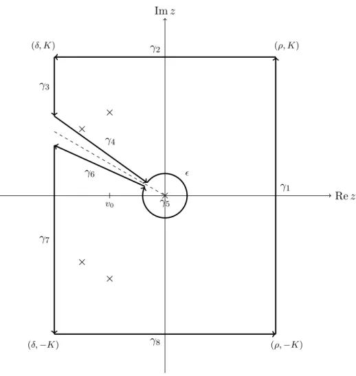
Proof. Case 1: δ <0.

We integrate the functionχ⁻¹_λ (z)e^zt along the keyhole contourγ =γ₁∪. . .∪ γ8, as shown in Figure 1, with vertices (ρ, K),(ρ,−K),(δ,−K) and (δ, K), where ρ >kAk^1/α. Due to the bounds in (5.1) and the fact that there are no accumulation points of N_A on C there are only finitely many zeros of

detχ_A inside the contour, independent of how large K and how small are chosen. We can also a find aϕ0 ∈(−π, π], |ϕ₀| ≥π/2 such that

{z=e^iϕ : (ϕ0−η < ϕ < ϕ0 or −2π+ (ϕ0+η)< ϕ <−2π+ϕ0), rcosϕ≥δ, r >0} ∩NA =∅ (5.4) for allη sufficiently small. We consider the function z^α with branch cut at ϕ=ϕ0.

γ1

γ₂ γ3

γ6

γ4

γ7

γ8

γ5

v0

Rez Imz

(ρ, K)

(ρ,−K) (δ, K)

(δ,−K)

Figure 1: Contour integration of χ⁻¹_λ (z)e^zt.

The residue theorem yields for every fixed t 1

2πi Z

γ

(χA(z))⁻¹e^ztdz = X

s∈Nn

Resz=s(χA(z))⁻¹e^zt).

Since we chose ρ to satisfy ρ > kAk^1/α, the integral along γ₁ tends to the fundamental solution asK → ∞:

R(t) = 1 2πi lim

K→∞

Z

γ1

(χ_A(z))⁻¹e^ztdz.

We show that the path integrals over γ₂ and γ₈ vanish as K → ∞, the limits of the integrals overγ3 and γ7 are decaying exponentially fort→ ∞, the limits of the path integrals over γ6 and γ4 decay polynomially in t for η→0 and →0. The integral overγ₅ depends on whereverA satisfies the condition (C1) or (C2). In the first case, it vanishes, in the latter case it converges polynomially intto the identity matrix.

Path integrals over γ2 and γ8

Let us consider the integral alongγ8. I₈:= 1

2πi Z

γ8

χ_A(z)⁻¹e^ztdz.

From the inequality (5.2) we know that χA is invertible for K^α > (1∨ e^{−τ δ})kAk. The Neumann series argument yields the following bound of the inverse function if we chooseK large enough:

kχ_A(z)⁻¹k=

z⁻¹

E_d−z^−α Z 0

−τ

e^zuA(du) −1

≤ |z|⁻¹ 1 1−

z^−αR₀

−τe^zuA(du)

≤ |z|^α−1

|z|^α−(1∨e^{−τ δ})kAk

≤ K^α−1

K^α−(1∨e^{−τ δ})kAk Therefore,

kI₈k ≤ Z ρ

δ

(χA(x−iK))⁻¹

e^xtdx≤ K^α−1

K^α−(1∨e^{−τ δ})kAk Z ρ

δ

e^xtdx

= K^α−1

K^α−(1∨e^{−τ δ})kAk

e^ρt−e^δt

t →0 forK→ ∞.

The same arguments hold for the integral alongγ2.

Integral along γ₅

Letz=e^iϑ, then dz=ie^iϑdϑ=iz dϑ.

I5:= 1 2πi

Z

γ5

1 z

E_d−z^−α Z 0

−τ

e^zuA(du) −1

e^ztdz

= 1 2πi

Z −π π

E_d−z^−α Z 0

−τ

e^zuA(du) ⁻¹

e^zti dϑ

We distinguish two cases. Let A[−τ,0] 6= 0 and det A[−τ,0] 6= 0. Then z^αEd−R0

−τe^zuA(du) → −A[−τ,0] for → 0. The dominated convergence theorem yields for every fixedt

kI₅k=

1 2πi

Z −π π

z^α

z^αEd− Z 0

−τ

e^zuA(du) −1

e^zti dϑ

≤c^αk(A[−τ,0])⁻¹ke^cost→0 for→0

with a constant c independent of t. Let A[−τ,0] = 0. The first term in the Taylor series expansion of the integral vanishes and it holds that R₀

−τe^zuA(du) =P∞ k=1z^kR₀

−τ u^k

k!A(du) and E_d−z^−α

Z 0

−τ

e^zuA(du)→E_d for→0. (5.5)

Applying again the dominated convergence theorem we obtain I₅→ 1

2πi Z −π

π

E_di dϑ=−E_d. Integrals along the paths γ3 and γ7

Letz=δ+iy. withy1 =δtan(ϕ0−η), y2=δtan(ϕ0+η) it holds that I_3,7= 1

2πi Z

γ3∪γ₇

χ⁻¹_A (z)e^ztdz

= 1 2π

Z _y1

K

χ⁻¹_A (z)e^ztdy+ 1 2π

Z −K y2

χ⁻¹_A (z)e^ztdy

= 1 2π

Z y1

K

χ⁻¹_A (z)−(z−vn+1)⁻¹E_d e^ztdy + 1

2π Z −K

y2

χ⁻¹_A (z)−(z−v_n+1)⁻¹E_d e^ztdy + 1

2π Z y1

K

(z−v_n+1)⁻¹E_de^ztdy+ 1 2π

Z −K y2

(z−v_n+1)⁻¹E_de^ztdy

It holds that

K→∞lim lim

η→0

1 2π

Z _y1

K

(z−v_n+1)⁻¹e^ztdy+ 1 2π

Z −K y2

(v_n+1−z)⁻¹e^ztdy

E_d

=

− 1 2π

Z ∞

−∞

(z−v_n+1)⁻¹e^ztdy

E_d=−e^vn+1tE_d.

The last equality holds due to the fact that the Laplace transform ofx7→e^ax is equal to _z−a¹ .

Let us now consider the first term in the representation ofI_3,7: 1

2π Z y1

K

χ⁻¹_A (z)−(z−vn+1)⁻¹E_d e^ztdy

= 1 2π

Z y1

K

χ⁻¹_A (z)(z−v_n+1)⁻¹E_d

e^zt((z−v_n+1)E_d−χ_A(z)) dy.

Let

x= min{|δ−Rez| :z∈N_A}.

Then |δ +iy−z| ≥ x > 0 for all z ∈ N_A and all y ∈ IR₊. Hence there exists a constant c > 0 such that kχ_A(δ +iy)k ≥ c for all y ≥ δtanϕ0. The integral R₀

−τe^(δ+iy)uA(du) is bounded along the path γ₃ and hence kχ_A(δ+iy)kk(v_n+1−δ−iy)E_dkbehaves asymptotically likey² fory→+∞:

kχ_A(δ+iy)kk(δ+iy)−v_n+1k ≥c₁(1 +y²)

with a constant c₁ independent of t. On the other hand k(z−vn+1)Ed−χA(z)k ≤ |v_n+1|+|z|^1−αk

Z 0

−τ

e^zuA(du)k ≤c2(1 +y^1−α).

Hence e^−δt

1 2π

Z y1

K

χ⁻¹_A (z)−(z−vn+1)⁻¹E_d e^ztdy

≤e^−δt Z ∞

0

c₂(1 +y^1−α)

c₁(1 +y²) e^δtdy≤ Z ∞

0

c₃ 1

1 +y^1+αdy <∞.

The second term in the representation of I_3,7 is treated analogously. Thus, sup_t>0e^−δt|I_3,7|<∞, sincee^(vn+1−δ)t is bounded for allt.

Integrals along the paths γ4 and γ6

We investigate the asymptotic properties of I4,6:= 1

2πi Z

γ4∪γ₆

χ⁻¹_A (z)e^ztdz

asη and tend to zero simultaneously. We will need η to converge to zero quicker than and choose therefore η =ⁿ, n > k0, where k0 is defined as in (5.3). We show

A satisfies (C1): sup_t>0lim→0t^αI_4,6<∞.

A satisfies (C2): sup_t>0lim→0t^k0−αI_4,6<∞.

Onγ4 and γ6 we set

z=re^i(ϕ0−η), ≤r ≤δ/cos(ϕ0−η), z˜=re^i(ϕ0+η), ≤r ≤δ/cos(ϕ0+η), z^α=|z|^αeⁱargzα=r^αe^{i(ϕ0−η)α}, z˜^α =|˜z|^αeⁱarg˜zα−2πiα =r^αe^{i(ϕ0+η)α−2πiα}, and write

I4,6= 1 2πi

Z

δ/cos(ϕ0−η)

1

z(Ed−z^−α Z 0

−τ

e^zuA(du))⁻¹e^zte^i(ϕ0−η)dr + 1

2πi

Z δ/cos(ϕ0+η)

1

˜

z(E_d−z˜^−α Z 0

−τ

e^zu˜ A(du))⁻¹e^zt˜e^i(ϕ0+η)dr.

We study the behaviour of the integrated functions in the neighbourhood of zero and on the intervalI± = [0, δ/cos(ϕ0 ±η)] separately: I4,6 = I>0 + I<0, where

I_>0 =− 1 2πi

Z

I−

χ⁻¹_A (z)e^zte^i(ϕ0−η)dr+ 1 2πi

Z

I+

χ⁻¹_A (˜z)e^˜zte^i(ϕ0+η)dr, I<0 =− 1

2πi Z 0

χ⁻¹_A (z)e^zte^i(ϕ0−η)dr+ 1 2πi

Z 0

χ⁻¹_A (˜z)e^zt˜e^i(ϕ0+η)dr.

For any fixed 0 > 0 the norms of the inverse matrices are bounded for z∈I±. Moreover, applying the dominated convergence theorem we obtain

kI_>0k ≤c

Z δ/cosϕ0

e^rtcosϕ0dr=ce^δt−e^tcosϕ0

tcosϕ₀ , (5.6)

where c depends only on ₀. So,kI_>0k decays to zero at exponential rate fort→ ∞.

Remark 5.1. Letα= 1/2,τ = ^{log 3}₂ and A=

1{−τ} −2·1{0}

2·1_{0} −1_{−τ}

. It holds that

detχA(z) =z^1−α(4−3^z−z) and detχA(−1) = 0,

hence the norms of the inverse matricesχ_A(z), χ_A(˜z) would be not necessary bounded in the limit if we chose the negative real line segment for the path integralsγ4 and γ6. A ϕ0 satisfying (5.4) guarantees the bound in (5.6).

Let us now consider the behaviour of the integrand for ₀ small enough.

LetA satisfy (C1). For0 sufficiently small it holds that kz^αE_d−

Z 0

−τ

e^zuA(du)k → kA[−τ,0]k.

Hence, kχ_A(z)⁻¹k behaves like r^α−1 for r ≤ 0. There exists a constant c >0, independent oft and0 such that

kI_<0k ≤ Z 0

0

cr^α−1e^rcosϕ0tdr

=c(−cosϕ0)^−αt^−α(Γ(α)−Γ(α,−t₀cosϕ0))≤ct^−α, where Γ(α, y) is given by

Γ(α, y) :=

Z ∞ y

x^α−1e^−xdx, i.e., Γ(α)−Γ(α,−tδ) =

Z −tδ 0

x^α−1e^−xd^x→Γ(α), t→ ∞.

Hence, sup_t>0lim→0t^α(kI_<0k+kI_>0k) is finite.

More interesting is the case when A[−τ,0] = 0. In this case the norms of the integrals along γ4 and γ6 tend to infinity, but they cancel. This is due to the fact that the only terms which include fractional powers ofz tend to zero as ₀ and η tend to zero, so the integrals cancel due to the opposite sign. Let us first consider the integrated function alongγ4.

From (5.5) we have for allr≤₀, where₀ is chosen to be sufficiently small,

E_d−z^−α Z 0

−τ

e^zuA(du)

| {z }

A1(z)

−E_d(1−c₁z^k0−α)

| {z }

B1(z)

≤c₂r^k0+1−α.

The constantsc₁ and c₂ are independent of r and . Hence,

A⁻¹(z)

z −B⁻¹(z) z

≤ kA⁻¹(z)kkB⁻¹(z)kc₂r^k0−α ≤c3r^k0−α,

sinceA⁻¹(z), B⁻¹(z) converge to the identity matrix asz→0. Same results

hold also on γ₆ with constants ˜c₁,c˜₂,c˜₃. Moreover,

B⁻¹(z)

z −B⁻¹(˜z)

˜ z

=

E_d

1

z(1−c₁z^k0−α) − 1

˜

z(1−c˜₁z˜^k0−α)

≤

e^i(ϕ0+η)−e^i(ϕ0−η) r

+c₄r^k0−α−1

=

e^iϕ0(e^iη−e^−iη) r

+c4r^k0−α−1

2e^iϕ0sinη r

+c₄r^k0−α−1

≤c5rⁿ⁻¹+c4r^k0−α−1≤c6r^k0−α−1. We obtain

kI_<0k ≤ Z 0

A⁻¹(z)

z −A⁻¹(˜z)

˜ z

e^rcosϕ0tdr

≤ Z ₀

A⁻¹(z)

z −B⁻¹(z) z

+

A⁻¹(˜z)

˜

z −B⁻¹(˜z)

˜ z

+

B⁻¹(z)

z −B⁻¹(˜z)

˜ z

e^rcosϕ0tdr

≤ Z 0

((c3+ ˜c3)r^k0−α+c6r^k0−α−1)e^rcosϕ0tdr

−→→0 c₇(−tcosϕ₀)^α−k0(Γ(k₀−α)−Γ(k₀−α,−₀tcosϕ)).

Case 2: δ >0.

Forδ >0 we only need to consider the rectangle contour with vertices with (ρ, K),(ρ,−K),(δ,−K) and (δ, K). Again, the integrals along γ₂ and γ₈ vanish as K → ∞, where the path integral over (δ, K) → (δ,−K) grows

asymptotically at exponential ratee^δt.

Example 5.1. The case where A[−τ,0]6= 0, but detA[−τ,0] = 0 is more complicated. Let us consider the following example. Letd= 2 and

A=

1_{−τ} −1_{−τ1} 1_{−τ1} −1_{−τ}

,

where 0< τ1 < τ. It holds that detA[−τ,0] =−1 + 1 = 0.

B(z) :=z^αE_d− Z ₀

−τ

e^zuA(du) =

z^α−e^{−τ z} e^−τ1z

−e^−τ1z z^α+e^{−τ z}

and

detB(z) =z^2α−det Z 0

−τ

e^zuA(du) =z^2α−

∞

X

k=1

akz^k

with somea_k∈IR.

B⁻¹(z) = 1

detB(z)adj B(z) = 1 z^2α−P∞

k=1akz^k

z^α+e^{−τ z} −e^−τ1z +e^−τ1z z^α−e^{−τ z}

. The adjugate of B(z) converges to a constant non-zero matrix for z → 0 andz^α−1det¹B(z) behaves likez^β, whereβ <−1. Hence, the path integrals overγ5,γ4 and γ6 diverge, whereas the other integrals tend to zero.

Let us now consider A=

1_{−τ} 1_{−τ1} 1_{−τ1} 1_{−τ}

, Then

detB(z) =z^2α−z^α(e^{−τ z}+e^{−τ z}) + det Z 0

−τ

e^zuA(du).

The adjugate of B(z) again converges to a constant non-zero matrix for z→0 and z^α−1det¹B(z) behaves likez⁻¹. Hence, the path integral over γ₅ converges to the identity matrix and the path integralsγ₄ and γ₆ cancel.

6 Conclusions

In the present paper, we study the asymptotic properties of the fundamental solution fractional delay differential equations. First, the results on existence and uniqueness of solutions of FDDEs are proved. Based on the character- istic function and characteristic equation, several interesting properties of the solution are obtained. We are able to present a complete picture of the asymptotic behaviour in a very general setting, which includes many cases studied in literature.

References

[1] Y. Chen and K. L. Moore. Analytical stability bound for a class of de- layed fractional-order dynamic systems. Nonlinear Dynamics, 29:191–

200, 2002.

[2] K. Diethelm and N.J. Ford. Multi-order fractional differential equations and their numerical solution. Appl. Math. Comput., 154.

[3] K. Diethelm and N.J. Ford. Analysis of fractional differential equations, 2002.

[4] A. Erd¨elyi et al. Higher Transcendental Functions, Vol III. McGraw- Hill, New York, Toronto, London, 1953.

[5] C. Hwang and Y.-C. Cheng. A numerical algorithm for stability testing of fractional delay systems. Automatica, 42:825–831, 2006.

[6] S.M. Verduyn Lunel J.K. Hale. Introduction to Functional Differential Equations. Springer, New York, 1993.

[7] A. A. Kilbas, H. M. Srivastava, and J. J. Trujillo. Theory and Applica- tions of Fractional Differential Equations, Volume 204 (North-Holland Mathematics Studies). Elsevier Science Inc., New York, NY, USA, 2006.

[8] U. K¨uchler and B. Mensch. On langevins stochastic differential equation extended by a time delayed term. Stochastics and Stochastic Reports, 40:123 – 144, 1991.

[9] M. P. Lazarevi´c. Finite time stability analysis ofpd^α fractional control of robotic time-delay systems. Mechanics Research Communications, 33(2):269–279, 2006.

[10] M. P. Lazarevi´c and A. M Spasi´c. Finite-time stability analysis of frac- tional order time-delay systems: Gronwall’s approach. Mathematical and Computer Modelling, 49(3-4):475 – 481, 2009.

[11] K.B. Oldham and J. Spanier. The Fractional Calculus: Theory and Application of Differentiation and Integration to Arbitrary Order. Aca- demic Press, New York, 1974.

[12] S. Samko, A. Kilbas, and O. Marichev.Fractional Integrals and Deriva- tives: Theory and Applications. Gordon and Breach, London, 1993.

[13] C. Li W. Deng and J. Lu. Stability analysis of linear fractional differen- tial system with multiple time delays.Nonlinear Dynamics, 48:409–416, 2007.

[14] X. Zhang. Some results of linear fractional order time-delay system.

Applied Mathematics and Computation, 197(1):407 – 411, 2008.