Bidding Behavior in Asymmetric Auctions: An Experimental Study ¤
Werner Güth Radosveta Ivanova-Stenzel Elmar Wolfstetter
Abstract
We review an asymmetric auction experiment. Based on Plum (1992) private valuations of the two bidders are independently drawn from distinct but commonly known distributions, one of which stochastically dominating the other. We test the qualitative properties of that model of asymmetric auctions, in particular whether the weak bidder behaves more aggressively than the strong and then test bidders’ preference for …rst- vs. second–price auctions.
JEL classi…cation: D44, C91
Keywords: Sealed Bid Auctions, Asymmetric Bidders, Private-Independent Values, Experiments
¤Humboldt-University of Berlin, Department of Economics, Spandauer Str. 1, D - 10178 Berlin, Germany; e-mail: {gueth,ivanova,wolf}@wiwi.hu-berlin.de - This paper is part of the EU-TMR Research Network ENDEAR. Support from the Deutsche Forschungsgemeinschaft, SFB 373 (”Qunti…kation und Simulation ökonomischer Prozesse”), Humboldt-Universität zu Berlin, is gratefully acknowledged.
1. Introduction
Like most of the theoretical literature, auction experiments typically assume that bidders’ valuations or signals are drawn from the same probability distribution (see the survey by Kagel, 1995). However, this symmetry assumption is violated in many real-life auction environments, because bidders often know that and how they di¤er, for example, in the light of earlier experiences or due to collusion between subsets of otherwise symmetric bidders. The limited relevance of the symmetric auction framework is aggravated by the fact that many of the cele- brated results of symmetric auctions, such as the revenue equivalence of a larger class of auction games, do not extend to asymmetric auctions.
There is a small theoretical literature on asymmetric auctions, which deals with various kinds of asymmetries: asymmetries between commonly known distribution functions from which valuations or signals are independently drawn, asymmetries induced by a known ranking of valuations (which involves a particular stochastic dependency), and asymmetries between valuation functions while maintaining the symmetry of the distribution from which private signals are drawn.
Several authors have followed the …rst approach to model bidder asymmetry, and assumed that bidders’ valuations are independently drawn from di¤erent prob- ability distributions, which are common knowledge among them. In this spirit, Vickrey (1961) already considers an auction with two bidders in which the one bidder’s valuation is known to the other bidder with certainty, and Griesmer et al.(1967) analyze …rst-price auctions with two bidders whose valuations are uni- formly distributed over di¤erent supports.
More recently, Plum (1992) analyzes the two bidder case for arbitrary continuous distributions, and proves that the …rst-price auction has a unique pure strategy equilibrium with strictly monotone increasing bid functions. In addition, he ex- plicitly solves the …rst-price auction game for a parametric class of distribution functions.
In a similar framework, Maskin and Riley (2000a) explain the properties of several asymmetric two bidder examples, where a stochastic order stronger than …rst- order stochastic dominance is assumed, Maskin and Riley (2000b), Reny (1999), and Simon and Zame (2000) analyze existence of pure strategy equilibria in …rst- price auctions for the generalnbidder case, and Lebrun (1999) proves uniqueness of pure strategy equilibria in the general nbidder case.1
Asymmetries induced by a known ranking of valuations are analyzed by Lands- berger et al.(2000). This asymmetry cannot be subsumed under the approach that assumes that valuations are independently drawn from commonly known distribution functions. And indeed, it generates distinct results.
Another branch of the literature has also begun to analyze asymmetries between valuations functions in the a¢liated and (almost) common-value framework, while maintaining the symmetry of the distribution from which private signals are drawn (see the example by Bikchandani (1988), and the associated experiment by Avery and Kagel (1998); see also the example by Bulow, Huang, and Klemperer (1999)).
In the literature there are only a few asymmetric auction experiments. Most of them concern the common-value case (see the survey by Kagel, 1995). Employ- ing the private-value framework Pezanis-Christou (1999) tests one variant of the Maskin and Riley model (2000a) and rejects the predicted revenue ranking.
The present paper reports on a laboratory experiment of bidding behavior in asymmetric auctions, which assume that valuations are private information and are independently drawn from distinct but commonly known distribution func- tions. The experiment employs the functional speci…cation used by Plum (1992) and Kalkofen and Plum (1996) for which explicit equilibrium solutions of bid- ding strategies are available. We explore whether actual bidding exhibits similar qualitative properties as the game-theoretic solution. In particular, we ask:
1Incidentally, these proofs of existence employ very di¤erent methods. Maskin and Riley (2000b) use topological methods developed by Dasgupta and Maskin (1986). Plum (1992) and Lebrun (1999) establish directly that a solution to a suitable set of di¤erential equations exists.
And Reny (1999) employs his concept of “payo¤ secure” games. Finally, Simon and Zame (2000) view the tie-breaking rule as part of the solution of the game, and show that there is always some tie–breaking rule for which an equilibrium exists.
² Does the weak bidder bid more aggressively than the strong bidder?
² Does the …rst–price auction raise more expected revenue for the seller?
² Does the second–price auction generate higher payo¤s to the strong bidder and the …rst-price auction to the weak bidder?
² Do bidders rank the two auctions accordingly?
² Can deviations from equilibrium strategies be explained by caution or risk aversion?
In the experiment each subject played either the role of the weak or the strong bidder, and this for 6 rounds of bidding in a …rst–price auction and another 6 rounds in a second–price auction. The 1st phase consisted of 4 cycles of such 12 bidding rounds. Subjects confronted randomly selected partners in match- ing groups of 14 participants, namely 7 bidders 1 and 7 bidders 2. Thus each participant confronted altogether 7 co-bidders in an irregular fashion.
Do both bidders understand which auction yields higher payo¤s, as unambigu- ously predicted by theory? To explore this question, the second phase of an experimental session introduces an additional stage. Before learning their private values participants must determine a price limit for dictating the pricing rule.
The second phase consists of 16 successive such auction games. Due to incentive compatibility of random pricing (see Becker, De Groot, and Marschak, 1963) and of random dictatorship our mechanism should induce participants to reveal their true willingness to pay for choosing the pricing rule.
At the end of the experiment participants play another 16 rounds (third phase) where they choose their price limits after learning their private values.
The remainder of the paper is organized as follows. The theoretical background and the experimental design are explained in Sections 2 and 3. In Section 4 we present the main experimental results. We close with the summary of the results in Section 5.
2. Theoretical background
We consider a slightly simpli…ed version of Plum (1992). Speci…cally, two risk- neutral bidders(i= 1;2)compete for the purchase of a single item in either a …rst–
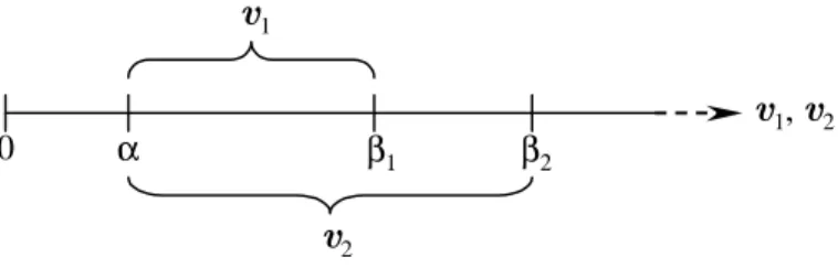
or a second–price sealed–bid auction. Bidders’ valuations are private information and independently drawn from uniform distributions with supports [®; ¯1] and [®; ¯2], with
¯2 = 200> ¯1 = 150> ®= 50; (2.1) as illustrated in Figure 1. Therefore, the random valuation V2 is obtained by
“stretching” the valuation V1. Obviously, V2 is more favorable than V1, in the strong sense of …rst–order stochastic dominance.
0 α β1 β2
v1
v2
v1, v2
Figure 1: Support of random valuations
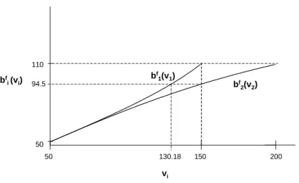
Equilibrium bid functions As shown by Plum (1992, pp. 401–403), the …rst–
price sealed–bid auction has the following equilibrium bid functions:
bfi(vi) =®+ vi¡® 1 +p
1 +°ic(vi¡®)2 for i= 1;2 (2.2) with c:= 1
(¯1¡®)2 ¡ 1
(¯2¡®)2 (2.3)
°1 :=¡1; °2 := 1: (2.4)
These are plotted in Figure 2, which shows that the bidder with the more favorable valuation (bidder 2) bids pointwise less than bidder 1. An immediate implication is that the …rst-price auction gives rise to ine¢ciency, because the bidder with the lower valuation wins the auction with positive probability. (For example, if v2 = 150, the bidder with the lower valuation wins the auction for all V1 in (130.18,150), as illustrated in Figure 2).
50 150 200 110
50
vi
bfi(vi) bf1(v1)
bf2(v2)
130.18 94.5
Figure 2: Equilibrium bid functions in …rst-price sealed-bid auction
Of course, truthful bidding is an equilibrium in dominant strategies in the second–
price sealed–bid auction, and so is the following plausible modi…cation of truthful bidding which assumes that bidder 2 will never bid more than his rival’s maximum valuation ¯1:
bsi(vi) =
½ vi ifvi ·¯1
¯1 ifvi 2[¯1; ¯2] (2.5)
Bidders’ equilibrium payo¤s Using Plum’s solution of the two auction games, one can compute bidders’ equilibrium payo¤s, denoted byui(vi). These are needed as a benchmark in our experiment.
If the auction is second–price sealed–bid, the computation ofusi(vi)is straightfor- ward. By a well–known resultusi0(vi) =Fj(vi), therefore:
us1(v1) = Z v1
®
F2(x)dx and (2.6)
us2(v2) =
½ Rv2
® F1(x)dx if v2 ·¯1 R¯1
® F1(x)dx+v2¡¯1 if v2 2[¯1; ¯2] (2.7) If the auction is a …rst–price sealed–bid auction, biddersi’s equilibrium probability of winning the auction is
Pr³
bfi(vi)> bfj(Vj)´
= Pr³
Vj < bfj¡1(bfi(vi))´
(2.8)
= Fj
³bfj¡1(bfi(vi))´
(2.9) Therefore, in order to compute ufi(vi), one needs to …nd the inverse Ái(x) of the equilibrium bid function which is de…ned on bids x, as follows:2
Ái(x) := bfi¡1(x) =®+ 2(x¡®)
1¡°i(x¡®)2c: (2.10) Therefore, one obtains:
ufi(vi) :=Fj(Áj(bfi(vi)))(vi¡bfi(vi)) (2.11)
= vi¡bfi(vi)
¯j¡®
à 2(bfi(vi)¡®) 1¡°j(bfi(vi)¡®)2c
!
: (2.12)
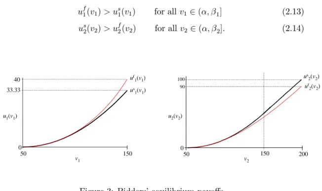
Bidders’ equilibrium payo¤s are plotted for both auction rules in Figure 3 which il- lustrates that the strong bidder 2 strictly prefers the second-price auction, whereas the weak bidder 1 strictly prefers the …rst-price auction:
uf1(v1)> us1(v1) for allv1 2(®; ¯1] (2.13) us2(v2)> uf2(v2) for allv2 2(®; ¯2]: (2.14)
50 150
40
0
uf1(v1) us1(v1) 33.33
v1 u1(v1)
100 90
0
50 150 200
v2 u2(v2)
uf2(v2) us2(v2)
Figure 3: Bidders’ equilibrium payo¤s
2In order to …nd the inverse of equilibrium bid functions, employ the following transformation:
Bi := bi¡®, xi := vi ¡®, di := p
1 +°icx2i, and one obtains, after a few manipulations, xi = 2Bi=(1¡°iBi2c).
These completely opposite rankings are intuitively appealing, and they are con- sistent with a key result in Maskin and Riley (2000a).
Bidders’ equilibrium payo¤s behind the veil of ignorance From the ui(vi)’s one can compute bidders’ equilibrium payo¤s behind the veil of ignorance, i.e., the expected payo¤s determined before valuations are drawn:
Uis:=E[usi(Vi)] = 1
¯i¡®
¯i
Z
®
usi(x)dx (2.15)
Uif :=Eh
ufi(Vi)i
= 1
¯i¡®
¯i
Z
®
ufi(x)dx: (2.16)
For the assumed values of the parameters®,¯i this implies:
U1s = 11:111< U1f = 12:295 (2.17) U2s = 36:111> U2f = 32:474. (2.18)
Of course, this ranking is implied by (2.13)-(2.14).
Bidders’ value of dictatorship behind the veil of ignorance In the ex- periment (2nd phase) we give bidders the chance to select the auction rule, before they know their valuation. Speci…cally, we let them bid for the right to choose the favored auction against a random price generator (Becker, De Groot, Marschak, 1963) If the bid is at or above that random price, the bidder must pay the random price and dictatorially chooses his favored auction rule, otherwise the auctioneer selects the auction rule by the ‡ip of a fair coin.
Obviously, truthful bidding is the optimal strategy and the value of the right to choose the auction, which we call value of dictatorship,L, is de…ned as follows:
Li = maxn
Uis; Uifo
¡ 1
2(Uis+Uif) (2.19) L1 = 0:592<1:8185 =L2: (2.20)
Of course, if the bidder gains „dictatorship”, he chooses the auction that gives the higher Ui. As one can see from (2.17)-(2.18), the weak bidder 1 prefers the
…rst-price auction whereas the strong bidder 2 favors the second–price auction. In view of L2 > L1 the same random price generator applied to bidder 1 and 2 will less often induce dictatorial rule choices in case of bidder 1.
Value of dictatorship if bidders know their valuation In the experiment (3rd phase) we also give bidders the chance to select the auction rule after learning their valuation, i.e., after the veil of ignorance has been removed, again using the random price mechanism. In the spirit of Li one may de…ne the value of dictatorship as follows:
li(vi) = maxn
usi(vi); ufi(vi)o
¡ 1
2(usi(vi) +ufi(vi)): (2.21) However, this ignores some subtle updating and strategic signalling issues. For example, in the event when the strong bidder 2 fails to dictate the preferred second-price format, player 1 should update his probability assessment ofv2, which in turn a¤ects the equilibrium strategies of the subsequent …rst-price auction game and hence the equilibrium payo¤ufi(vi)in (2.21). Therefore, (2.21) can only serve as a rough benchmark, if at all.
3. Experimental design
In the experiment we neither excluded over- nor underbidding by lettingv1 vary from 50 to 150 and v2 from 50 to 200 whereas bids bi(vi) could vary from 0 to 250. The random price p of the 2nd (3rd) phase was chosen from the range 0 ·p · 30 since the value of the right to dictate the pricing rule should always be non-negative. Of course, neither vi nor bi(vi) can vary continuously in a computerized setup. Actually both,vi andbi had to be integers. The two private values v1 and v2 were independently drawn form a uniform distribution with support f50;51; :::;150g, respectivelyf50;51; :::;200g:.
A session was subdivided into three phases:
The 1st Phase consisted of 4 cycles of 12 bidding rounds, …rst 6 rounds with the …rst-price rule, then 6 rounds of the second-price rule. In each round …rst the private valuesv1 andv2were randomly selected. Then the two bidders determined their bidb1(v1), respectivelyb2(v2).
The 2nd Phaseconsisted of 16 bidding rounds with endogenous price rule. First both, bidder i = 1 and bidder i = 2, had to state their price limit li for being able to dictate the pricing rule (F or S). It was then determined by an unbiased chance move whether 1 or 2 became the potential dictator. If this was bidder i, he could dictate the pricing rule F or S whenever the randomly chosen price d of dictatorship with 0· d · 30 satis…ed d ·li. After choosing F or S the auction round was played as in the 1st phase.
The 3rd Phase di¤ered from the 2nd phase only by the timing of events.
Here …rst the private values v1 and v2 were randomly selected, i.e., all decisions (li, F or S, bi)were made knowing one’s private value vi.
The bidders were informed whether or not they have bought, about the price to be paid by the buyer, their private (reselling) value, their own bid, the bid of the other bidder, their own payo¤ in the current round, their total pro…t up to this time and their average pro…t in each auction type. At the end of each auction in phase 2, respectively 3, the dictator also learned about his costs for choosing the pricing rule.
Participants were invited to register for the experiment (mainly by distributing lea‡ets in undergraduate courses of the economics faculty of Humboldt Univer- sity in Berlin). After entering the computer laboratory participants were seated at visually separated terminals where they could read the instructions (see Ap- pendix B). They could privately ask for clari…cations but not for advice. We have performed 8 sessions, 7 with 14 participants and 1 with 12 participants each (due to a technical problem only the results of the 1st phase could be saved for one of the 8 sessions). All sessions lasted about two hours.
4. Results
In the following, we use the theoretical results of Section 2.2 as a benchmark to assess the actual bidding behavior in phases 1 and 2. The analysis of phase 3 is primarily of an exploratory nature since the associated theoretical benchmark is debatable.
4.1. E¢ciency, prices and bidders’ pro…ts
Despite the assumed asymmetry, the second-price auction is e¢cient, since truth- ful bidding is an equilibrium in dominant strategies. However, the …rst-price auction give rise to ine¢ciency, because the bidder with the lower valuation wins with positive probability (see Figure 2). In the experiment we measure e¢ciency (I) as follows:
I = vbuyer maxfv1; v2g
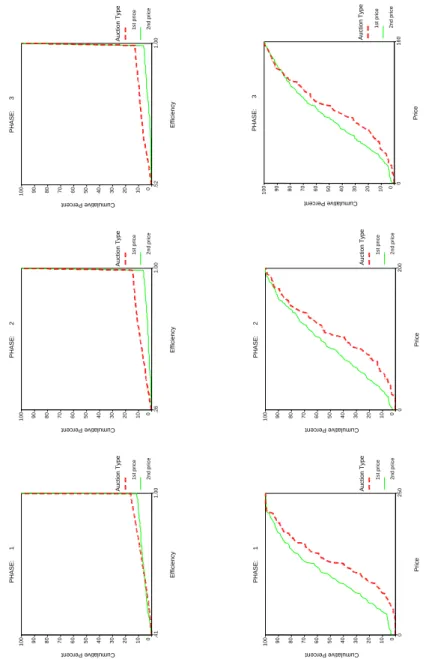
Although there is a slight ine¢ciency of second-price auctions, it is, however, lower than the one of the …rst-price auction (see Figure A.1 and Table ”Summary Statistics” in Appendix A).
price rule …rst-price second-price 1 .97 (84%) .98 (88%) phase 2 .97 (85%) .99 (94%) 3 .98 (87%) .99 (94%) Table 1: Average degreeI of e¢ciency (in brackets: Percentage of Pareto-e¢cient allocations)
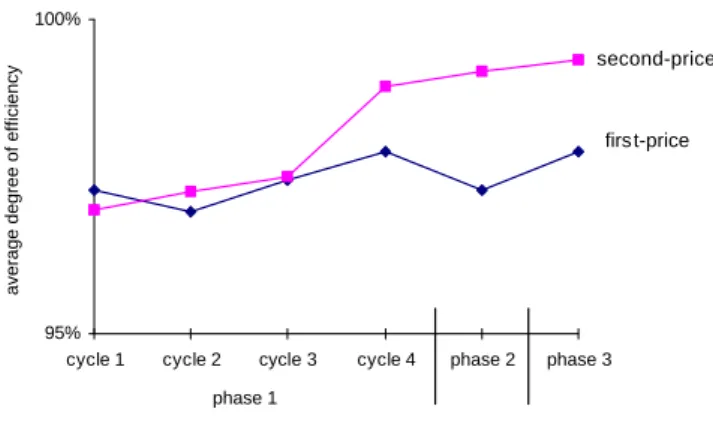
Learning to induce e¢cient allocations is more pronounced in second-price auction than in …rst-price auction when measured by phases (see Table 1). As shown in Figure 4 we observe on average a stable increase of e¢ciency in second-price auctions over time. The greater ine¢ciency of …rst-price auctions results from the need to coordinate how far one should underbid one’s private value, i.e., how large the positive di¤erence vi¡bi(vi) should be.
95%
100%
cycle 1 cycle 2 cycle 3 cycle 4 phase 2 phase 3
average degree of efficiency
phase 1
second-price
firs t-price
Figure 4: Average degree I of e¢ciency over time
Let us assume the perspective of the seller who is interested in a large expected revenue. Table 2 lists in the top row the expected equilibrium prices p¤ (see Kalkofen and Plum, 1996) and in the lower rows the average prices of the …rst- and second-price auction, separately for phase 1, 2, and 3.3 A Binomial test (p = :004; one-tailed, N = 8, phase 1)4 for all three phases reveals that the seller’s revenues from …rst-price auctions are higher than those from second-price auctions (see Table ”Summary Statistics” in Appendix A). The cumulative dis- tribution function for second-price auction is in all three phases above that one for …rst-price auction (see Figure A.1 in Appendix A). Note that according to the realized prices in phases 1 and 2 the incentive of the seller for the …rst-price rule is substantially larger than indicated by the solution prices for risk-neutral bidders, i.e., the theoretic solution underestimates the actual advantage of relying on …rst- rather than on second-price auctions.
price rule …rst-price second-price normative 90.46 88.89
1 103.87 87.06
phase 2 104.70 90.69
3 98.74 89.97
Table 2: Expected/average prices
3Of course, these benchmark prices can only be used as a rough approximation in the analysis of phase 3.
4For phases 2 and 3: p=:008(N = 7):
According to Table 3 the mean pro…ts for both bidders are higher for the second- price auction than for the …rst-price auction. Whereas the payo¤s in phases 1 and 2 of the second-price auction are close to their benchmarks in all sessions5, in the
…rst-price auction they are invariantly below their benchmarks (2.17)-(2.18). The second-price auction generates signi…cantly higher payo¤s to the bidders, both weak and strong, and in all three phases.6 The possibility to endogenously select the auction type in the 2nd (3rd) phase leads to no essential earning e¤ects.7
bidder 1 2
price rule …rst-price second-price …rst-price second-price
1 6.37 11.23 22.75 35.36
phase 2 6.65 11.12 21.68 34.42
3 7.35 11.72 22.15 33.83
Table 3: Average bidders’ pro…ts
4.2. Bidding behavior
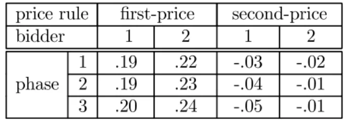
In Table 4 we compare the average level of under/over-bidding [vi¡bi(vi)]=vi
for …rst- and second-price auction as well as for the di¤erent phases and the two bidders, forvi 2 f50;51; :::;150g.
price rule …rst-price second-price
bidder 1 2 1 2
1 .19 .22 -.03 -.02
phase 2 .19 .23 -.04 -.01
3 .20 .24 -.05 -.01
Table 4: Average under/overbidding
5We have con…rmed that the distributions of actually selected valuesv1andv2 do not di¤er signi…cantly from the a priori-distributions.
6One-tailed Binomial test; for phase 1: p=:004 (N = 8);phase 2: p=:008 (N = 7), phase 3: p=:062 (N = 7):
7In phase 2 and 3 this includes, of course, the costs resulting from the random price mecha- nism, i.e., the earnings from bidding are slightly higher when being able to dictate the auction type.
According to Table 4 under/overbidding ratios are rather stable (over phases).
The average tendency in second-price auctions seems to be truthful bidding, i.e., bi(vi) = vi for i = 1;2. Nearly half of all bids in all three phases are equal to subjects’ reselling values (39% in phase 1, 47% in phase 2, and 48% in phase 3).
Possible reasons for the revealed slight overbidding could be that:
- the dominant strategy is not transparent;
- spite on behalf of bidder 1 (who overbids more often and who might feel underprivileged);
- sealed-bid procedures mays slow down learning, since they frequently do not provide the feedback that tends to reduce overbidding.
As to be expected, …rst-price auctions rely on substantial underbidding (see Table
”Summary Statistics” in Appendix A). The mean degree of underbidding in the range50·vi ·150is signi…cantly larger for bidder 2 than for bidder 1 (p=:035;
one-tailed Binomial test, N = 8, phase 1).8
0,00 0,05 0,10 0,15 0,20 0,25 0,30 0,35 0,40 0,45 0,50
50-60 61-70 71-80 81-90 91-100 101-110 111-120 121-130 131-140 141-150 151-160 161-170 171-180 181-190 191-200
bidder 2
bidder 1
vi
optimal degree of underbidding vi-b*(vi)
vi
0,00 0,05 0,10 0,15 0,20 0,25 0,30 0,35 0,40 0,45 0,50
50-60 61-70 71-80 81-90 91-100 101-110 111-120 121-130 131-140 141-150 151-160 161-170 171-180 181-190 191-200
bidder 2
bidder 1
vi
median actual degree of underbidding vi-b(vi)
vi
Figure 5: Degree of underbidding in …rst-price auction (phase 1)
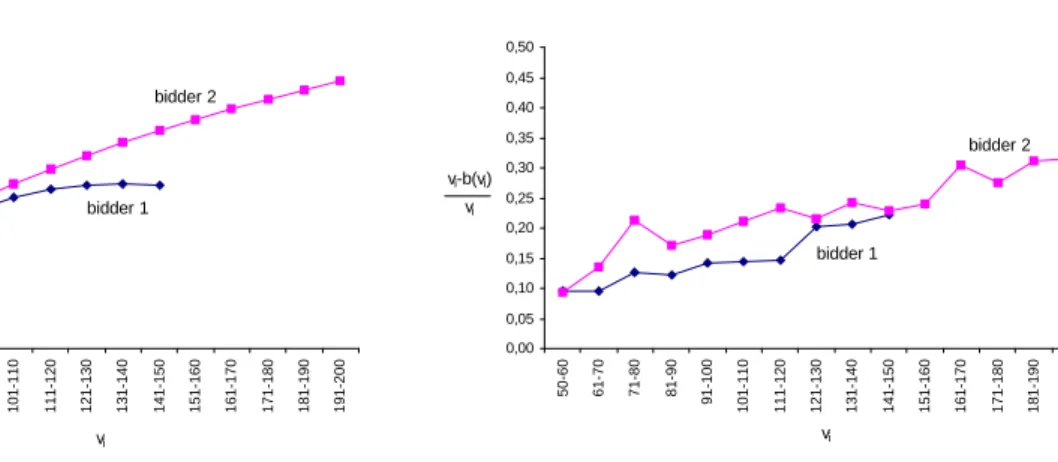
For …rst-price auction it is interesting to analyze how the degree of underbidding depends on vi. In Figure 5 the left diagram illustrates the optimal degree of
8For phases 2 and 3 in 5, respectively 6, out of 7 sessions we observe larger underbidding for bidder 2.
underbidding[vi¡b¤i (vi)]=vi fori= 1;2and the right diagram the median actual (underbidding) results for both bidders in phase 1.9 The equilibrium as well as the observed bids are computed as the average bids for the respectivevi-brackets.
Two qualitative aspects of the left diagram seem to hold also for the right one, namely the same underbidding degree by bidder 1 and 2 for v1 =v2 = 50 and a general tendency of bidder 1 to underbid less.
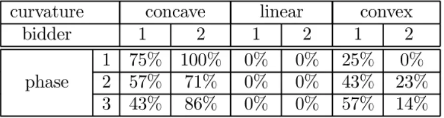
Let us now investigate the curvature of the observed …rst-price bid functions for both bidder types. To evaluate whether the bid functions were increasing and convex, concave or linear we estimated the following piecewise linear regression model:
bi =½i+±ivlowi +°ivhighi (i= 1;2), with (4.1)
v1low =
½ v1 if v1 <100
100 otherwise , vlow2 =
½ v2 if v2 <125 125 otherwise vhigh1 =
½ v1 ¡50 if v1 ¸100
50 otherwise , v2high=
½ v2¡75 if v2 ¸125 50 otherwise
Thus we allow for a kink at v1 = 100, respectively v2 = 125 (the mean values of vi; i = 1;2).10 This can provide piecewise-linear approximations of convex or concave bid functions. Model (4.1) was estimated for each session and each phase separately, giving us a total of 22 estimated bid functions per bidder’s type. The
…t of these piecewise-linear approximations is reasonable: in 75% (33 out of 44 observed bid functions) the estimated individual bid function explained 70% or more of the variance (R2 ¸0:7).
In all cases the bid functions were strictly increasing, i.e., ±i > 0 and °i > 0 (i = 1;2). To determine the curvature of the bid functions we computed the
9The corresponding mean degrees of underbidding are similar but, due to outliers, slightly less regular.
10A slightly simpler formulation of a piecewise–linear regression model may be: bi = ¾i +
¸ivi+¹ivihighwith all variables as de…ned above. However, this model is equivalent to model 1, and the latter is better suited to compare±i and°i below. For instance, if a bid function is perfectly linear, this results in±i=°i:
di¤erence between the two slope coe¢cients ¢i ´ °i ¡±i, i = 1;2: We consider a bid function as linear if j¢ij · §0:01:11 If ¢i < ¡0:01 (¢i > +0:01); the respective bid function is classi…ed as concave (convex). Due to these criteria in all three phases there are no linear bid functions (see Table 5). For both bidders most of them are concave (except for bidder 1 in phase 3).
curvature concave linear convex
bidder 1 2 1 2 1 2
1 75% 100% 0% 0% 25% 0%
phase 2 57% 71% 0% 0% 43% 23%
3 43% 86% 0% 0% 57% 14%
Table 5: Curvature of the estimated …rst-price bid functions
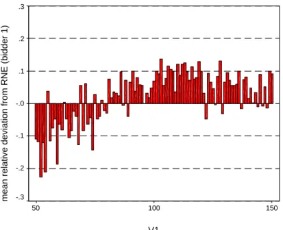
We also analyze for …rst-price auctions the relative bid deviations from the risk neutral equilibrium (RNE) bidding strategyb¤i(vi), namely[bi(vi)¡b¤i (vi)]=vi for i = 1;2 and both phases, 1 and 2. There are no signi…cant di¤erences for both bidders: For bidder 1 65% of all bids in phase 1 (66% in phase 2) are above the benchmark, for bidder 2 the share is 67% (respectively 67%). A Binomial test rejects the null hypothesis of no deviations in favor of the weak overbidding prediction, i.e., there is a positive relative deviation from RNE (p = :035; one- tailed, N = 8, phase 1).12
Most bids below the benchmark result from low reselling values, i.e., if vi < 100 (see Figures A.2 and A.3 in Appendix A).13 The share of negative deviations in phase 1 decreases nearly by half when increasing private values. A Spearman correlation analysis reveals no clear-cut correlation between the absolute relative deviations from RNE and the rounds.
11Admittedly, the chosen criterion for linearity is ad hoc. It could have been set less (or more) restrictively. Even if the criterion for linearity is set less restrictively, e.g. j¢ij · §0:02, i.e.
the prediction area has been doubled compared to the criterion we report here, only one bid function for bidder 2 in the 2nd phase would be considered as linear.
12For phase 2 in 6 out of 7 sessions the (weak) overbidding prediction is valid.
13The coexistence of negative (mainly for low vi-values) and positive (mainly for high vi- values) deviations from risk-neutral bidding indicates that such deviations are not only due to risk aversion.
4.3. Price limits
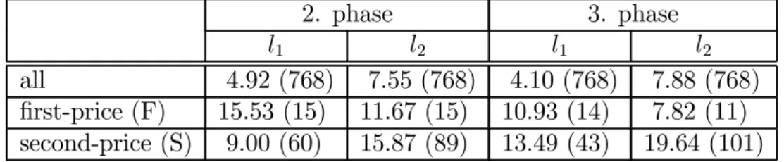
Table 6 gives the average price limits l1 and l2 for phases 2 and 3 …rst for all participants, then separately for those who, as actual dictator, have chosen the
…rst- (game F) or the second-price rule (game S). The number in brackets are the number of observations on which these averages rely. The equilibrium price limits of risk-neutral bidders behind the veil of ignorance, i.e., before bidders know their private valuations (see the results in Section 2.2) are
L1 = 0:592 and L2 = 1:8185
In phase 3 where bidders 1 and 2 know their private valuesv1 andv2, respectively, the actual and observed price limits should, of course, depend on these values.
2. phase 3. phase
l1 l2 l1 l2
all 4.92 (768) 7.55 (768) 4.10 (768) 7.88 (768)
…rst-price (F) 15.53 (15) 11.67 (15) 10.93 (14) 7.82 (11) second-price (S) 9.00 (60) 15.87 (89) 13.49 (43) 19.64 (101) Table 6: Average price limits separately for phase 2/3 and for F/S-dictators14
According to Table 6 in the second phase bidders 2 on average choose higher price limits (l2) than bidders 1 (l1), as suggested by L1 and L2. We have checked for phase 2 that bidders 1 and 2 had nearly equal chances to become the random dictator. Therefore, the observed higher frequency with which bidder 2 dictates the auction mechanism (104=75) can be attributed to the fact that the higher average price limit of bidder 2 translates into a higher chance to win against the random price generator.
14For phase 3 the price limits are (simply) the averages of all price limits li(vi) for all 16 rounds and randomly chosenvi-levels.
Both bidders reveal considerably higher willingness to pay for dictating the price rule than predicted by theory (see also Table ”Summary Statistics” in Appendix A). Remarkable is the fact that for the weak bidders in phase 2 the average price limit of F-voters exceeds the one of S-voters. Although this is consistent with the theoretical result that the weak bidder should prefer the …rst-price auction, it is, however, puzzling that the average price limits are so much higher than the theoretical predictions.
Also both bidders have predominantly chosen game S which may be due to the fact that it makes bidding easier. Besides, the second-price auction yielded higher average pro…ts than the …rst-price auction for 75% of the weak bidders and 88%
of the strong bidders in the …rst phase of the experiment.
bidder 1 2
value vi v1 ·100 v1 >100 v2 ·125 v2 >125
…rst-price (F) 50% 50% 45% 55%
second-price (S) 19% 81% 18% 82%
Table 7: Frequency of F/S, chosen in phase 3, depending on the mean value of vi
By Table 7 we can investigate in more detail how choosing the pricing rule during the 3rd phase depends on whethervi is above its mean value 100, respectively 125, or not. The large majority of S-voters have private values in the upper vi-range, while for F-voters the two vi-ranges have (nearly) equal frequencies.
Whereas during phase 2 both price limits, l1 and l2, on average decrease over time (Figure A.4 in Appendix A), this e¤ect is much weaker for phase 3 (see Figure A.5 in Appendix A where, for the sake of comparability, we only look at price limits li(vi) for vi in the 30 width-interval around its mean). This smaller decline in phase 3 seems to be mainly due to lower starting values l1 and l2. At the beginning of phase 2 participants were apparently too enthusiastic about the possibility of dictating the pricing rule.
For phase 3 we have split up the price limits l1 and l2 into its two, respectively three 50 width-intervals [50;100], (100;150], (150;200]. The data reveal that larger valuesvi trigger on average larger price limitsli (see Figures A.6 and A.7 in Appendix A). As shown by Figures A.8 and A.9 (see Appendix A) for the range [50;100], respectively (100;150] the price limits of bidders 1 and 2 with nearly equal values are very close. Actually comparing thel1- andl2-distribution for the two intervals reveals no signi…cant di¤erence.
5. Concluding remarks
Although auctions are a familiar topic in experimental economics, most experi- ments deal with the case of symmetry. Our experiment studies auctions where private valuations are independently drawn from distinct but commonly known distributions, one of which …rst-order stochastically dominates the other. Our results (phase 1 and 2) support the theoretical prediction that a seller should be better o¤ choosing the …rst-price than the second-price auction as well as other qualitative properties of the game-theoretic solution. More speci…cally we observe:
² prices are signi…cantly higher in a …rst-price auction
² in …rst-price auctions the strong bidders bid far less than weak bidders
² in …rst-price auctions, bid functions are nonlinear
² in second-price auctions, bids are close to bidders’ valuations
² strong bidders set, on average, higher price limits
² the weak bidders who opt for the …rst-price auction set, on average, higher price limits than those who opt for the second-price format.
These results con…rm that the predictive power of the asymmetric auction model is reasonably good, despite the complexity of the bidding problem. Given the fail- ure of revenue equivalence in experimental studies of the symmetric independent private values model, the world of asymmetric auctions seems to be an interesting and promising area for further research.
References
[1] Avery, C., and Kagel, J. H. (1998): Second-price auctions with asymmetric payo¤s: An experimental investigation, Journal of Economics and Manage- ment Strategy, 6, 576-603.
[2] Becker, G. M., M. H. De Groot, and J. Marschak (1963): An experimental study of some stochastic models for wagers,Behavioral Science, 8, 41 - 55.
[3] Bikchandani, S. (1988): Reputation in repeated second-price auctions,Jour- nal of Economic Theory, 46, 97-119.
[4] Bulow, J., Huang, M., and Klemperer, P. (1999): Toeholds and takeovers, Journal of Political Economy, 107, 427-454.
[5] Dasgupta, P., and Maskin, E. (1986): The existence of equilibrium in dis- continuous economic games, I and II, Review of Economic Studies, 53, 1-26, 27-41.
[6] Griesmer, J. M., Leviatan, R. E., and Shubik, M. (1967): Towards a study of bidding processes,Naval Research Quarterly, 14, 415-433.
[7] Kagel, J. H. (1995): Auctions: A survey of experimental research, in: Hand- book of experimental economics, J. H. Kagel and A. E. Roth (eds.), Princeton, New Jersey: Princeton University Press, 501 - 585.
[8] Kalkofen, B., and M. Plum (1996): Optimal pricing-rules for private-value auctions with incomplete information, ifo Studien, 42, 77 - 100.
[9] Landsberger M., J. Rubinstein, E. Wolfstetter and S. Zamir (2000), First- Price Auctions when the Ranking of Valuations is Common Knowledge, Re- view of Economic Design, forthcoming.
[10] Lebrun, B. (1999): First price auctions in the asymmetric n bidder case, International Economic Review, 40, 125-142.
[11] Maskin, E. S. and J. G. Riley (2000a), Asymmetric auctions, Review of Eco- nomic Studies, 67, 413-438.
[12] Maskin, E. S. and J. G. Riley (2000b), Equilibrium in sealed high bid auction, Review of Economic Studies, 67, 439–454.
[13] Pezanis-Christou, P. (1999): On the Impact of Low-Balling: Experimental Results in Asymmetric Auctions, mimeo: Laboratory for Experimental Eco- nomics, University of Bonn
[14] Plum, M. (1992): Characterization and computation of Nash-equilibria for auctions with incomplete information, International Journal of Game The- ory, 20, 393 - 418
[15] Reny, P. (1999): On the existence of pure and mixed strategy Nash equilib- rium in discontinuous games, Econometrica, 67, 1029-1056.
[16] Simon, L. K., and Zame, B. W. R. (2000): Cheap talk and discontinuous games (mimeo), Econ. Dept., UCLA.
[17] Vickrey, W. (1961): Counterspeculation, auctions, and competitive sealed tenders,Journal of Finance, 16, 8-37.
Appendix A:
PHASE: 1 Efficiency
1.00.41
Cumulative Percent
100 90 80 70 60 50 40 30 20 10 0
Auction Type 1st price 2nd price
PHASE: 2 Efficiency
1.00.26
Cumulative Percent
100 90 80 70 60 50 40 30 20 10 0
Auction Type 1st price 2nd price
PHASE: 3 Efficiency
1.00.52
Cumulative Percent
100 90 80 70 60 50 40 30 20 10 0
Auction Type 1st price 2nd price PHASE: 1 Price
2500
Cumulative Percent
100 90 80 70 60 50 40 30 20 10 0
Auction Type 1st price 2nd price
PHASE: 2 Price
2000
Cumulative Percent
100 90 80 70 60 50 40 30 20 10 0
Auction Type 1st price 2nd price
PHASE: 3 Price
1600
Cumulative Percent
100 90 80 70 60 50 40 30 20 10 0
Auction Type 1st price 2nd price
Figure A.1: Cumulative distributions of the observed e¢ciency and prices (for both auction types)
V1
150 100
50
mean relative deviation from RNE (bidder 1)
.3
.2
.1
-.0
-.1
-.2
-.3
Figure A.2: Relative bid deviation from RNE (bidder 1, …rst-price auction, phase 1)
V2
200 125
50
mean relative deviation from RNE (bidder 2)
.3
.2
.1
-.0
-.1
-.2
-.3
Figure A.3: Relative bid deviation from RNE
(bidder 2, …rst-price auction, phase 1)
0.00 2.00 4.00 6.00 8.00 10.00 12.00 14.00 16.00
1 2 3 4 5 6 7 8 9 10 11 12 13 14 15 16 round t
price limits (l1,l2) on average
l2
l1
Figure A.4: Time paths of price limits (l1; l2) in phase 2
0.00 2.00 4.00 6.00 8.00 10.00 12.00 14.00 16.00
1 2 3 4 5 6 7 8 9 10 11 12 13 14 15 16 round t
price limits (l1,l2) on average
l2
l1
Figure A.5: Time paths of price limits (l1; l2) in phase 3 (price limits li(vi)only for vi in 30 width-interval around its mean)
0.00 5.00 10.00 15.00 20.00 25.00 30.00
1 2 3 4 5 6 7 8 9 10 11 12 13 14 15 16 round t
price limit l1 on average
v1∈[50,100]
v1∈(100,150]
Figure A.6: Time paths of price limit l1 for v1 2[50;150] in phase 3
0.00 5.00 10.00 15.00 20.00 25.00 30.00
1 2 3 4 5 6 7 8 9 10 11 12 13 14 15 16 round t
price limit l2 on average
v2∈(150,200]
v2∈(100,150]
v2∈[50,100]
Figure A.7: Time paths of price limit l2 for v2 2[50;200] in phase 3
0.00 5.00 10.00 15.00 20.00 25.00 30.00
1 2 3 4 5 6 7 8 9 10 11 12 13 14 15 16 round t
price limits (l1,l2) on average
l1 l2
Figure A.8: Time paths of price limits (l1; l2) for v1; v2 2[50;100] in phase 3
0.00 5.00 10.00 15.00 20.00 25.00 30.00
1 2 3 4 5 6 7 8 9 10 11 12 13 14 15 16 round t
price limits (l1,l2) on average l2
l1
Figure A.9: Time paths of price limits (l1; l2) forv1; v2 2(100;150] in phase 3
auction type phase All
1 2 3 4 5 6 7 8
mean efficiency rate first price 1 0.97 0.97 0.97 0.98 0.96 0.98 0.98 0.98 0.97
2 0.97 0.97 0.98 0.98 0.97 - 0.96 0.97 0.98
3 0.98 0.97 0.98 0.99 0.96 - 0.97 0.99 0.99
second price 1 0.98 0.97 0.97 0.97 0.98 0.98 0.98 0.99 0.97
2 0.99 0.99 0.99 0.99 1.00 - 1.00 1.00 0.98
3 0.99 0.99 1.00 0.99 1.00 - 1.00 1.00 0.99
percentage of first price 1 84.1% 84.5% 81.0% 85.4% 80.4% 85.1% 87.5% 86.3% 82.7%
pareto opt. allocations 2 85.1% 80.7% 92.9% 84.4% 86.1% - 86.7% 81.4% 85.4%
3 87.2% 84.1% 85.5% 95.9% 79.4% - 83.3% 91.7% 88.0%
second price 1 88.4% 87.5% 86.9% 85.4% 90.5% 89.3% 90.5% 92.9% 83.9%
2 93.5% 92.7% 92.9% 92.2% 93.4% - 95.5% 97.1% 90.6%
3 93.9% 91.2% 96.5% 93.6% 97.4% - 95.3% 93.8% 88.1%
mean price first price 1 103.87 103.80 108.86 101.93 92.80 107.93 106.89 107.84 100.65 2 104.70 103.51 103.79 103.25 95.00 - 108.02 106.47 110.48 3 98.74 98.61 104.27 102.63 77.21 - 100.15 102.21 98.92 second price 1 87.06 83.82 93.65 90.61 70.18 88.68 89.74 89.02 91.29 2 90.69 88.49 95.19 94.23 72.58 - 90.00 94.62 102.13 3 89.97 96.75 92.32 96.19 74.76 - 88.16 92.33 94.26
std. dev. first price 1 25.80 27.62 28.52 21.06 22.20 26.35 24.86 23.66 27.04
(mean price) 2 26.52 28.40 23.36 27.98 27.84 - 29.39 23.65 23.62
3 26.25 27.79 24.89 21.57 25.58 - 25.98 24.05 27.48 second price 1 33.79 33.01 29.95 33.67 46.36 30.72 29.35 26.14 32.22 2 33.78 32.75 30.07 29.51 45.16 - 28.80 23.89 33.59 3 32.09 27.87 24.37 27.55 41.09 - 28.17 27.61 35.91 mean under/overbidding first price bidder 1 1 0.19 0.21 0.12 0.18 0.36 0.14 0.11 0.14 0.22
(v-b)/v for v ∈[50,150] 2 0.19 0.18 0.11 0.16 0.51 - 0.06 0.12 0.21
3 0.20 0.27 0.15 0.19 0.38 - 0.13 0.14 0.21
bidder 2 1 0.22 0.25 0.17 0.23 0.33 0.18 0.15 0.20 0.27
2 0.23 0.29 0.17 0.24 0.37 - 0.19 0.13 0.21
3 0.24 0.23 0.18 0.21 0.51 - 0.22 0.17 0.25
second price bidder 1 1 -0.03 -0.03 -0.06 -0.10 0.20 -0.03 -0.07 -0.04 -0.10
2 -0.04 -0.07 -0.06 -0.09 0.14 - -0.05 -0.05 -0.17
3 -0.05 -0.10 -0.06 -0.07 0.09 - -0.03 -0.09 -0.16
bidder 2 1 -0.02 0.10 -0.12 0.00 0.09 -0.16 -0.05 -0.05 0.02
2 -0.01 0.05 -0.11 -0.07 0.15 - -0.03 -0.08 0.02
3 -0.01 -0.03 -0.10 -0.07 0.14 - 0.01 -0.04 -0.05
std. dev. first price bidder 1 1 0.20 0.24 0.15 0.11 0.27 0.12 0.19 0.13 0.19
(mean und./overbid.) 2 0.27 0.14 0.09 0.10 0.32 - 0.47 0.09 0.18
3 0.17 0.23 0.10 0.12 0.25 - 0.07 0.10 0.18
bidder 2 1 0.20 0.20 0.21 0.12 0.24 0.15 0.18 0.13 0.23
2 0.20 0.20 0.20 0.19 0.20 - 0.11 0.11 0.26
3 0.20 0.17 0.16 0.16 0.20 - 0.13 0.09 0.26
second price bidder 1 1 0.30 0.26 0.29 0.33 0.41 0.30 0.29 0.12 0.24
2 0.24 0.10 0.14 0.12 0.35 - 0.23 0.08 0.32
3 0.23 0.24 0.16 0.11 0.29 - 0.15 0.11 0.33
bidder 2 1 0.31 0.30 0.35 0.21 0.31 0.35 0.23 0.20 0.39
2 0.28 0.23 0.32 0.26 0.40 - 0.15 0.14 0.27
3 0.23 0.13 0.24 0.24 0.31 - 0.11 0.11 0.26
mean price limits bidder 1 2 4.92 8.35 4.67 2.78 3.48 - 7.40 4.15 3.28
3 4.10 4.10 3.08 3.53 6.02 - 5.64 2.97 3.28
bidder 2 2 7.55 7.79 6.79 4.83 11.29 - 4.64 9.89 7.23
3 7.88 8.63 9.51 6.24 9.69 - 7.00 8.69 5.16
median price limits bidder 1 2 2.00 4.00 3.00 1.00 4.00 - 5.00 0.50 1.00
3 1.00 3.00 0.00 0.50 4.00 - 1.00 0.00 0.00
bidder 2 2 5.00 10.00 5.00 3.00 13.50 - 2.00 8.00 5.00
3 4.00 5.00 3.00 1.00 6.00 - 4.50 6.50 0.00
std. dev. bidder 1 2 6.62 8.84 6.20 5.06 3.71 - 8.06 5.71 5.02
(price limits) 3 6.49 5.18 6.07 5.47 7.04 - 8.02 5.03 7.28
bidder 2 2 7.39 6.64 7.41 5.42 8.00 - 5.73 7.40 8.18
3 9.53 9.71 10.86 9.08 10.49 - 9.00 8.88 7.57
Session
Summary Statistics
Appendix B:
Instructions
15:Phase 1:
Please, read these instructions carefully. They are identical for all participants.
During the experiment you will take part in several auctions. In every auction a
…ctitious commodity is for sale which you can resell to the experimenters. You are one of two bidders. In each auction there are two bidders, 1 and 2, with di¤erent value ranges [50;150] and [50;200]. Each participant belongs either to type 1 or to type 2 and keeps his own type during the entire experiment. Both bidders know for sure the both value ranges. In every auction the private reselling value v of each bidder is independently drawn from the interval 50 · v1 · 150 for bidder 1 and from the interval 50· v2 · 200 for bidder 2, respectively, with every integer number between 50 and 150 for bidder 1 and between 50 and 200 for bidder 2, respectively, being equally likely. Each bidder may place integer bids in the range from0to250. The bidder with the highest bid buys the commodity and pays a price according to the pricing rule. Then he sells the commodity to the experimenter and receives his reselling value. The other bidder does not pay anything and does not receive anything. If the both bids are equal, the buyer is chosen randomly (by the ‡ip of a fair coin).
There are two di¤erent types of auction. In …rst-price auction the price is the highest bid. In second-price auction the price which has to be paid is the second highest bid. We denote by bw the highest and by b2w the second highest bid.
First-Price Auction:
- Price = highest bid (p=bw)
15This is a translated version of the instructions. For the original instructions (in German), please contact one of the authors.
- Bidder with highest bid becomes buyer. He pays p.
- Pro…t of buyer: vw¡p - Pro…t of non-buyer: 0
Second-Price Auction:
- Price = second highest bid (p=b2w)
- Bidder with highest bid becomes buyer. He pays p.
- Pro…t of buyer: vw¡p - Pro…t of non-buyer: 0
In each auction the bidder groups are formed randomly. After you have placed your bid you are informed whether or not you are the buyer, about the price, which has to be paid by the buyer, your private reselling value, your own bid, the bid of the other bidder, how much you have earned in this auction, your total pro…t up to this time and your average pro…t in each auction type (per auction type). Altogether, you will play 48 successive auctions, which consist of 4 cycles of 12 bidding rounds. In one cycle each participant plays …rst 6 times the …rst-price auction and then 6 times the second-price auction.
All values are denoted in a …ctitious currency termed ECU for Experimental Currency Unit. The exchange rate from ECU to DM is: 100 ECU = DM 1:50.
You receive an initial endowment of DM 10.50 (700 ECU) to cover possible losses.
Any decision you make is anonymous and cannot be related to you personally by your co-bidders. If you have questions, please, raise your hand. We will then clarify your problems privately.
Phase 2 and 3:
You now will play another 32 auctions. By the …rst 16 auctions (phase 2) the bidders can choose the auction type according to the following rules: Both bidders