The Elasticity of Substitution between Clean and Dirty Energy with Technological Bias

(1)

Research Collection

Working Paper

The Elasticity of Substitution between Clean and Dirty Energy with Technological Bias

Author(s):

Jo, Ara

Publication Date:

2020-10

Permanent Link:

https://doi.org/10.3929/ethz-b-000447726

Rights / License:

In Copyright - Non-Commercial Use Permitted

This page was generated automatically upon download from the ETH Zurich Research Collection. For more information please consult the Terms of use.

(2)

CER-ETH – Center of Economic Research at ETH Zurich

The Elasticity of Substitution between Clean and Dirty Energy with Technological Bias

A. Jo

Working Paper 20/344 October 2020

Economics Working Paper Series

(3)

The Elasticity of Substitution between Clean and Dirty Energy with Technological Bias

Ara Jo

^∗

October 13, 2020

Abstract

The elasticity of substitution between clean and dirty energy and the direction of technological change are central parameters in discussing one of the most challenging questions today, climate change. Despite their importance, there are few studies that empirically estimate these key parameters. In this paper, I estimate the elasticity of substitution between clean and dirty energy from micro data, jointly with technological parameters that reflect the direction of technological change within the energy aggregate. I find estimates of the elasticity of substitution ranging between 2 and 3. The largely dirty-energy- biased technological change observed in the data validates the framework of directed technological change, given the historical movement of relative energy prices and the estimated elasticity of substitution above unity. However, I also find suggestive evidence that clean-energy-augmenting technology is growing faster than dirty-energy-augmenting technology in recent years with changes in relative energy prices and higher subsidies for clean energy.

Keywords:Elasticity of substitution, directed technical change, climate change.

JEL Classification:Q40, Q55, Q54, O33.

∗Center of Economic Research, ETH Zürich, Zürichbergstrasse 18, 8089 Zürich, Switzerland.

Email: ajo@ethz.ch. I thank Alexandra Brausmann, Miguel León-Ledesma, Giovanni Marin, Mar- ianne Saam, and Francesco Vona and participants at RESEC seminar, EAERE 2020 conference, KEEA 2020 conference and the International Workshop on Energy, Innovation and Growth for their helpful

(4)

1 Introduction

The elasticity of substitution between factors and the direction of technological change are critical parameters in many areas of economics. In environmental economics, a rich theoretical literature that investigates the possibility of sustainable growth through directed technological change has developed in response to climate change becoming one of the most challenging policy questions. In most of these models, the elasticity of substitution between clean and dirty energy plays a key role by determining the extent to which innovation efforts are encouraged towards the use of clean fuels, which ultimately allows sustainable growth (e.g. Otto et al., 2007; Ace- moglu et al., 2012; Fried, 2018; Greaker et al., 2018; Hart, 2019; Karydas and Zhang, 2019). Yet, there are few studies that empirically estimate these parameters, which leads to limited consensus on the magnitude of the elasticity of substitution and much less on the nature of technological change.¹ In this paper, I attempt to fill this gap in the literature by estimating the elasticity of substitution between clean and dirty energy inputs from micro data, jointly with technological parameters that capture the direction of technological change within the energy aggregate.

The importance of jointly estimating the elasticity of substitution and technological change is emphasized by the interconnectedness of the two parameters. To explain, the elasticity of substitution between inputs is captured by the percentage change in input ratios in response to a change in relative input prices. An increasing share of one input can occur when its relative price decreases. At the same time, it can be equally well explained by technological change biased towards or against that input depending on whether the two inputs are gross substitutes or comple- ments, respectively (Acemoglu, 2002). However, this interconnectedness makes it empirically challenging to separately identify the elasticity of substitution and the direction of technological change.

To tackle this problem, I use rich micro-level data from the French manufacturing sector. Using this data, I first develop stylized facts to motivate and inform the main estimation. First, there exists substantial heterogeneity in clean energy shares across

1For instance, for the elasticity of substitution between clean and dirty energy parameter in calibration, Otto et al. (2007) choose a value of 2 and Acemoglu et al. (2012) use 3 and 10 for the weak and strong substitutes scenario, respectively, while Karydas and Zhang (2019) choose a conservative benchmark value of 0.7 with a very different implication on the relationship between the two energy sources. Many of these studies also mention the difficulty of pinning down this parameter in their calibration due to a lack of empirical evidence.

(5)

firms within the same industry, which is not consistent with a constant factor share implied by a Cobb-Douglas relationship between clean and dirty energy sources.

This legitimizes the investigation of the elasticity of substitution between clean and dirty fuels. Further, the share of clean energy is positively correlated with overall energy efficiency at the firm level. This suggests the presence of non-neutral efficiency differences between clean and dirty energy and therefore encourages the specification of a separate technological progress parameter for each input in the estimation.

Motivated by these facts, I formulate a CES function of the energy composite that consists of clean and dirty energy with a separate technological parameter for each energy type.

Most existing studies estimate substitution parameters between production inputs (mostly labor and capital) based on the production function itself or on one of the first-order conditions (FOCs) of profit maximization. The estimation of the production function alone is generally only accomplished with restrictive assumptions about the nature of technological progress such as Hicks neutrality (Antras, 2004; León-Ledesma et al., 2010). In the environmental economics literature, a recent paper by Papageorgiou, Saam, and Schulte (2017) adopts this approach and provides the first empirical estimates of the elasticity of substitution between clean and dirty energy at the macro level assuming Hicks-neutral technological change.

On the other hand, the FOC approach does not allow identifying two separate technological progress parameters as will be explained later.

To overcome these limitations, I employ the system of equations approach that combines the production function and FOCs and exploits the parameter restrictions between the production and input demand functions. This approach allows me to estimate the elasticity of substitution between clean and dirty energy inputs as well as separate technological parameters that capture the direction of technological change within the energy aggregate. To the best of my knowledge, this paper is the first to provide joint empirical estimates for these key parameters with an explicit goal of making a clear connection to the theoretical literature.

I find micro estimates of the elasticity of substitution between clean and dirty energy inputs greater than unity, ranging between 2 and 3 as in a prior study (Pa- pageorgiou et al., 2017). The estimated technological progress parameters suggest the direction of technological change was largely biased towards dirty energy over the period of 1994 - 2015. The high (above unity) estimated elasticity of substitu-

(6)

tion, coupled with the relative price movement with dirty energy being considerably cheaper than clean energy throughout the sample period, rationalizes dirty- energy-biased technological change observed in the data from a theoretical stand- point. However, I also find suggestive evidence that government interventions had an impact on the direction of technological change – technological progress associated with clean energy occurred faster with the changes in relative prices and higher subsidies for clean energy in recent years.

These results provide a strong empirical foundation for a large number of studies that investigate the possibilities of sustainable growth with directed technological change in the presence of climate change (Otto et al., 2007; Acemoglu et al., 2012;

Golosov et al., 2014; Bretschger, 2015; Fried, 2018; Greaker et al., 2018; Borissov et al., 2019; Hart, 2019; Karydas and Zhang, 2019). The direction of technological change within the energy aggregate observed in the data validates the framework of directed technological change applied in the literature. The estimated dirty-energy- biased technological change especially in the early years of the sample is consistent with the prediction of the framework, given the historical movement of relative energy prices and the estimated elasticity of substitution above unity. Furthermore, most theoretical insights derived in the literature hinge on the assumption that the substitution elasticity between clean and dirty energy is sufficiently above unity.

The micro estimates for this key parameter presented in this paper provide empirical support for these models. Empirically, this paper is most related to Papageorgiou et al. (2017) that provides estimates for the elasticity of substitution between clean and dirty energy by estimating a nonlinear production function with neutral technological change. In the energy versus non-energy context, Hassler et al. (2012) jointly estimate the substitution parameter and the bias in the technological change and find a low (close to zero) elasticity of substitution between energy and non-energy inputs, although technological change seems to respond to strong price shocks such as the oil crisis in the 1970s.²

The article proceeds as follows. Section 2 develops a set of stylized facts from the data to motivate and inform the estimation. Section 3 derives estimating equations from a model of the firm’s energy use and Section 4 presents estimation results.

2This paper also relates to the large literature on interfuel substitution at a more disaggregate level (see Stern (2012) for a review). However, the goal of this paper differs considerably from that of this literature in that I attempt to estimate the elasticity of substitution using a binary distinction of clean and dirty energy (rather than disaggregate individual fuel types) along with the direction of technological change with an explicit goal of making a clear connection to the theoretical literature.

(7)

Section 5 concludes.

2 Stylized facts

2.1 Data

Data on the French manufacturing industry come from two main sources. First, the Enquête sur les Consommations d’Énergie dans l’Industrie (EACEI) administered by the French National Institute of Statistics and Economic Studies (Insee) provides plant-level information on energy use and expenditures by fuel. It covers a representative sample of manufacturing plants with at least 20 employees. Second, Fichier de comptabilité unifié dans SUSE (FICUS), also collected by Insee, provides information on firm characteristics such as industry, number of employees, date of creation and cessation, as well as detailed financial information including turnover, export, and operating costs.³ The FICUS covers the period between 1994 and 2007 and was replaced by the FARE in 2008.⁴ For the analysis that follows, I first aggregate the plant-level information from the EACEI to the firm-level and merge it with financial information from the FICUS and FARE in order to build an unbalanced panel of manufacturing firms that covers the period of 1994 - 2015. Given that the EACEI covers a sample of manufacturing plants, I only keep firm-year pairs for which all plants of a firm were surveyed in the EACEI to ensure that the aggregation of energy use and expenditure is comprehensive at the firm level.

I then aggregate energy use by fuel type to a clean and a dirty bundle for each firm. Following Papageorgiou et al. (2017), I add up electricity, steam and renewables into a clean aggregate and all other types (natural gas, petroleum products, etc) into a dirty aggregate.⁵ The French context offers a conceptual advantage in classifying electricity as a clean energy source, given that approximately 80 percent of electricity is produced by nuclear power and greenhouse gas intensities of nuclear power generation tend to be considerably lower than those of fossil technologies.⁶

3The Unified Corporate Statistics System (SUSE) is an annual fiscal census of manufacturing, mining and utilities firms on which the FICUS is based. SUSE covers all firms that are required to make tax declarations to the French Ministry of the Economy and Finance.

4The full name of the survey is Fichier approché des résultats d’Esane (FARE).

5Information on the use of renewable energy sources is included in the survey from 2005. Thus, up to 2004, only electricity and steam comprise the clean energy aggregate.

6Lenzen (2008) report that greenhouse gas intensity of nuclear power generation is between 10

(8)

[Table 1]

Energy purchase prices are deflated by the GDP deflator to reflect real prices.

The information on expenditure by fuel is similarly aggregated into a clean and a dirty energy expenditure. Using this information, I construct the average price measures for clean and dirty energy bundles by dividing the expenditure measures by corresponding consumption measures. Table 1 provides key descriptive statistics.

Using this data, below I develop a set of stylized facts from the descriptive statistics in order to motivate and inform the estimation that follows.

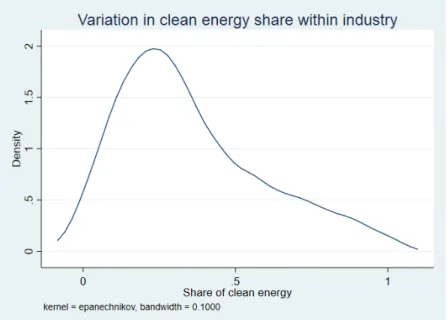
2.2 Within industry variation in clean energy shares

I first document substantial variation in the share of clean energy in the total energy consumption across firms within the same industry. As an example, Figure 1 presents the density of the clean energy share in the plaster, lime and cement industry that produces relatively homogeneous products through similarly homogeneous production process. We readily observe large heterogeneity in the clean energy share across firms. The median of the clean energy share distribution is 0.27.

Yet, about 25 percent of the firms in the industry have clean energy shares higher than 0.5.

[Figure 1]

Large dispersion in the clean energy share is observed across all industries. To have a sense of the degree of dispersion, I follow Raval (2019) and calculate 75th/25th and 90th/10th percentile ratios of the clean energy share distributions across firms for each industry. I then calculate the 25th percentile, the median, and the 75th percentile of these values across industries. Table 2 reports these results. For example, the clean energy share of the 75th percentile firm in the median industry is over 2.5 times that of the 25th percentile firm. Even in the 25th percentile industry, the 75/25 ratio is almost two, implying substantial heterogeneity in clean energy shares across all sectors in the economy. The variation is similar for the factor cost ratio, which is the ratio of the cost of clean energy to that of dirty energy.

[Table 2]

and 130 g CO2 per kWh, with an average of 65 g CO2 per kWh, which are significantly lower than those of fossil technologies (typically 600–1200 g CO2 per kWh).

(9)

A Cobb-Douglas relationship with the elasticity of substitution equal to unity would imply little variation in the share of clean energy (and in factor cost ratios), which is not consistent with the observed dispersion of clean energy shares across firms even within the same industry. This legitimizes the investigation of the elasticity of substitution between clean and dirty fuels in a CES representation.

2.3 Correlation with energy efficiency

Next, I explore whether overall energy efficiency of the firm, measured by revenue divided by the total amount of energy consumption, is correlated with the share of clean energy in the energy composite documented above. This will reveal whether there exists non-neutral efficiency differences between clean and dirty energy sources: if differences in energy efficiency are neutral and therefore affect both energy sources proportionately (as implied by a Cobb-Douglas relationship), these differences would not be correlated with factor shares. On the other hand, a correlation between overall energy efficiency and factor shares would suggest non-neutral efficiency differences between the clean and dirty energy sources.

As a starting point, I calculate the correlation coefficient between energy efficiency and the shares of clean energy across all firms and find the coefficient of 0.0184 significant at 1 percent level. I also check the role of age as a potentially im- portant determinant of the share of clean energy and find that younger firms tend to have higher shares of clean energy (with a correlation coefficient of -0.017 significant at 1 percent level).

[Table 3]

Next, I examine whether the correlation remains robust in regressions that include region and industry fixed effects, by regressing the share of clean energy on overall energy efficiency and a set of fixed effects as well as the firm’s age as a control. Table 3 reports these results. All regressions are weighted by the total energy consumption. Column (1) shows a strong positive association between the clean energy share and energy efficiency. I include age as a control in column (2) and find that it does not explain much variation in the share of clean energy any more.

The correlation between energy efficiency and the shares of clean energy remains statistically significant when region and industry specific factors are controlled for

(10)

(column (3)). These results point to the strong presence of non-neutral efficiency differences across different energy sources. Motivated by these stylized facts, I formulate a CES function of the energy composite that consists of clean and dirty energy with a separate technological parameter for each energy type.

3 Estimation strategy

I focus on how different sources of energy are combined and/or substituted in response to price signals and how efficiency associated with each energy type evolves, while abstracting away from the use of other production factors such as labor and capital. Formulating a production function with non-energy inputs as well as energy inputs necessitates imposing assumptions on the representation of these factors. For instance, for parsimony and tractability, previous studies have assumed the same elasticity of substitution between all inputs (Doraszelski and Jaumandreu, 2018; Raval, 2019) or a Cobb-Douglas relationship between some of the inputs (Pa- pageorgiou et al., 2017). However, existing empirical evidence suggests that the elasticity of substitution between labor and capital is significantly below unity (e.g.

Antras, 2004; Klump et al., 2007), while that between clean and dirty energy is likely to be above unity (Papageorgiou et al., 2017). Furthermore, Hassler et al. (2012) find that the elasticity of substitution between energy and non-energy inputs is not significantly different from zero (Hassler et al., 2012).⁷ All of this recent empirical evidence makes it unrealistic to assume the elasticity of substitution between labor, capital, clean and dirty energy (or just an energy aggregate) to be the same or to be one as implied by Cobb-Douglas between labor and capital or between energy and non-energy inputs. Thus, I abstract from other production factors and focus on the representative firm’s energy aggregate function:

E_it= [γ(A^c_itE_it^c)^σ−1^σ + (1−γ)(A^d_itE_it^d)^σ−1^σ ]^σ−1^σ (1) where E_it is the total energy consumption of firm i in year t, E_it^c and E_it^d are the consumption of clean and dirty energy, respectively. The key parameter of interest

7The authors estimate an aggregate production function with constant elasticity of substitution between energy (fossil fuels) and a composite of labor and capital using US data for the period of 1949- 2008. Given that their sample period is much longer than what is available for my analysis here, it is unlikely that the same elasticity would be larger in my context.

(11)

σrepresents the elasticity of substitution between the two types of energy. Follow- ing the literature in estimating production functions with factor-specific technological progress (David and Van de Klundert, 1965; Panik, 1976; Kalt, 1978; Antras, 2004; Klump et al., 2007; León-Ledesma et al., 2010), I assume the functional form of A^c_it=A^c₀e^τ^c^t, A^d_it=A^d₀e^τ^d^twhereτ_irepresents economy-wide growth in productivity associated with factori andt represents a time trend.⁸ Without loss of generality, the components of technological progress are scaled such thatA^c₀ = A^d₀ = 1. I also consider firm-specific technology in Section 4.2. The distribution parameter γ reflects the intensity of clean energy use. In what follows, I suppress the distribution parameter as in prior studies (Hassler et al., 2012; Papageorgiou et al., 2017), since it does not play a meaningful role in the estimation.

Most existing studies estimate substitution parameters between production inputs based on the production function itself or on one of the first-order conditions (FOCs) of profit maximization. The estimation of the production function alone is generally only accomplished with restrictive assumptions on the nature of technological progress such as Hicks neutrality. For instance, Papageorgiou et al. (2017) provides estimates for the elasticity of substitution between clean and dirty energy based on the nonlinear estimation of a CES production function that assumes neutral technological change. On the other hand, assuming that profit-maximising firms will set marginal products of inputs equal to their prices and that input markets are competitive, the FOC approach can be used to estimateσand the technological parameters. For instance, the standard log-linear FOC of profit maximization with respect toE_it^c yields:

log E_it

E_it^c

=a₁ + σ log P_it^c + (1−σ)τ_ct+_it (2) where a₁ is a constant. The limitation of this approach in my context is that there are two separate technological parameters. It would still be possible to have two separate technological parameters in the regression equation by combining the two FOCs with respect to each energy source as follows:

log E_it^d

E_it^c

=a₂+σ log P_it^c

P_it^d

+ (1−σ) (τ_c−τ_d)t+_it (3)

8Based on this approach, these studies provide evidence for labor-biased technological change, while simultaneously estimating the elasticity of substitution between labor and capital.

(12)

However, this specification would allow me to recover only overall biasτ_c−τ_d, rather than identifying the technological parameters separately.

To overcome these limitations, I employ the system of equations approach that combines the production function and FOCs:

log E_it^d

E_it^c

=a₂+σ log P_it^c

P_it^d

+ (1−σ) (τ_c−τ_d)t+_it (4) log E_it=a₃+ σ

σ−1log[(e^τ^c^tE_it^c)^σ−1^σ + (e^τ^d^tE_it^d)^σ−1^σ ] +µ_it (5) I include the combined FOCs in the system (equation (4)) rather than two separate FOCs with respect to each energy type in order to reduce omitted variable bias affecting both energy sources proportionately such as overall (factor-neutral) unob- served productivity or demand shocks experienced at the firm level. Such biases are expected to cancel out in the system and what remains is likely to be factor- specific omitted variable bias other than relative prices ^P_P^it^cd

it that affects fuel choices disproportionately.⁹ Later, I propose instruments to address factor-specific omitted variable bias such as heterogeneous factor-specific technology shocks across firms.

The system approach offers several advantages. First and foremost, it allows the joint identification of all parameters of interest: the elasticity of substitution between clean and dirty energy inputs as well as separate technological parameters that capture the direction of technological change within the energy aggregate. Second, from an economic perspective the system takes into account both profit-maximizing behavior of firms and technology expressed in the energy aggregate function. Finally, the estimation exploits the cross-equation restrictions between the production and input demand functions, which improves efficiency and the identification of technological progress parameters (Klump et al., 2007; León-Ledesma et al., 2010).

Firm fixed effects are not included throughout the analysis, since the primary goal is to provide estimates of key parameters from the theoretical literature that investigates theeconomy-widepossibility of sustainable growth through input substitution and directed technological change. Using only changes over time within firms

9Firm-level omitted variable biases that affect both energy bundles proportionately are likely to be innocuous also in equation (5), since the (log) CES representation specifies how fuel choice is de- terminedwithinthe energy aggregate through the degree of substitutability between the two energy sources and their relative efficiency. Factors that affect both energy sources proportionately would not affect either channel.

(13)

will lead to discarding changes in fuel prices that induce firms to adjust fuel choices at the extensive margin (i.e., start or stop using a certain energy type) or to close down.¹⁰ Thus, the estimates provided here incorporate fuel choices at the extensive margin and more generally entry, exit and the reallocation of inputs and production across firms. This also enables a meaningful comparison with results from earlier analysis at the industry level that incorporates input substitution across firms. To account for time-invariant and time-varying omitted variable bias, I instead rely on instruments. The system is estimated by the feasible generalized nonlinear least squares (FGNLS) method, accounting for possible cross equation error correlation (i.e., nonlinear variant of SUR). Standard errors are clustered at the firm level.

4 Results

4.1 Main findings

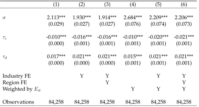
Table 4 reports the results from estimating the system of equations (4)-(5). The estimation is not weighted in the first three columns and weighted by the total energy consumption in the last three columns. Column (1) presents estimation results from estimating the system without any fixed effects. Note that, without any fixed effects, substitution in this specification encompasses many levels: across firms, industries, and regions and over time. The estimate of the elasticity of substitution between clean and dirty energy is well above unity around 2.1 and precisely estimated. The estimated technical progress parameters suggest -1% and 1.6% per year growth in the clean- and dirty-energy-augmenting efficiency, respectively.¹¹ The estimates indicate that technological change was clearly biased towards dirty energy over the period of 1994-2015.

[Table 4]

With industry fixed effects in column (2), the σ estimate falls slightly and yet remains close to 2. This is in line with substantial within-industry heterogeneity in

10In Section A1, I also provide within estimates of the elasticity of substitution and overall technological bias for comparison.

11A downward trend in efficiency is not infrequently found in factor-augmenting technology estimates. For instance, Antras (2004) and Doraszelski and Jaumandreu (2018) report negative estimates of capital-augmenting technology.

(14)

the share of clean energy across firms we have seen in Section 2.2. In column (3) also with region fixed effects, the estimated elasticity of substitution and technical progress parameters remain qualitatively the same. In column (4)-(6), I re-estimate the specifications in (1)-(3) using the total energy consumptionE_itas weights to put more emphasis on the behavior of heavy energy-using firms.σappear to be slightly higher for larger firms in all specifications. Technological progress estimates are comparable to the results from the non-weighted specification with 2 percent annual growth in efficiency associated with dirty energy (column (5) and (6)).

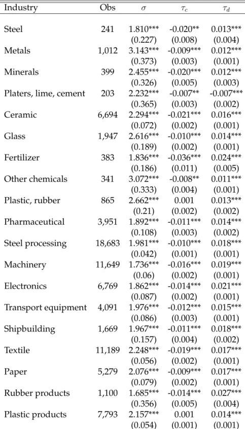
I further estimate the system by industry to examine how the parameters vary across industries based on the French classification of economic activities (NAF rev.2). Table 5 presents the results. Estimates of σ range between 1.6 and 3.1 and are precisely estimated for all industries. Technological parameters yield very similar results withτ_d positive andτ_cnegative in almost all industries. The implied bias in technological change,τ_d−τ_c, ranges between 1.3% and 5.1%.

[Table 5]

The general picture arising from these results largely confirms the theoretical predictions of the literature on endogenous technological change: the market size effect that encourages innovation in technologies that use the more abundant and cheaper input dominates the price effect that spurs the development of technologies that favor the more expensive input when the inputs are gross substitutes (σ >

1) (Acemoglu, 2002; Acemoglu et al., 2012). Figure 2 shows that the price of dirty energy was considerably lower than that of clean energy throughout the sample period. This relative price movement coupled with the estimated elasticity of substitution well over 1 rationalizes the dirty-energy-biased technological change observed in the data.

[Figure 2]

4.2 Addressing endogeneity

It is plausible that there exists factor-specific omitted variable bias that affects fuel choices disproportionately, which lead to biased estimates. For instance, following the literature in estimating production functions with factor-specific technological progress, the baseline specification is designed to capture the economy-wide direction of technological change. However, it is likely that there exists heterogeneity

(15)

in factor-specific technology at the firm level.¹² For instance, rather than a measure of economy-wide technological progress, A^c_t = e^τ^c^t and A^d_t = e^τ^d^t, one might consider A^c_it = e^τ^c^t+ξ^c^it, A^d_it = e^τ^d^t+ξ^d^it where ξ_it^c and ξ_it^d are unobservable factor-specific productivity at the firm level. This would imply that to the extent that firms take into account their factor-specific productivity when choosing inputs, it would affect relative input prices through input demands, leading to biased estimates.

To account for such firm-level heterogeneity in technology and endogeneity arising from it, I use Bartik-style instruments that apply the growth rates of energy prices at the national level to the initial firm-level price (Bartik, 1991). Relying on national growth rates of energy prices effectively blocks the channel through which factor-specific technology at the firm level influences relative prices through the firm’s relative input demands. A number of studies have used national energy prices in a similar way to address the endogeneity of firm-level energy prices and demand (e.g. Linn, 2008; Sato et al., 2019; Marin and Vona, 2019).¹³

Specifically, the instrument for the price of clean energyP_it^c,IV is constructed as follows:

12Doraszelski and Jaumandreu (2018) and Raval (2019) estimate technological progress at the firm level. However, following the tradition in the relevant literature, they clearly focus on the technological progress of one of the production inputs, namely, labor, with no separate specification for other factor-specific augmenting technology. This allows them to back out a measure of labor-augmenting productivity from the first-order condition. However, the goal of this paper is to separately and flexibly estimate technological progress parameters associated with clean and dirty energy. This leads to having two technological parameters in the first-order condition, which allows me to infer only overall bias in technological change. Thus, I mainly rely on the approach of using a time trend to proxy for economy-wide factor-specific technological progress, while trying to take into account potential endogeneity arising from heterogeneity in factor-specific technology across firms.

13These studies use the weighted sum of aggregate (e.g., national) fuel prices with time-invariant fuel share at the disaggregate (e.g., sector or firm) level as weights. Their instruments are similar to my specification in that they rely on national energy prices to block the channel through which sources of endogeneity such as technological change at the firm level affect energy prices through demand. The difference is that they retain firm-level (or sector-level) variation by using fixed firm- specific fuel shares as weights. This mitigates the concern of endogenous change in fuel mix due to technological change. In my context, however, changes in fuel mix are less worrisome since energy is already partitioned into the clean and dirty bundle with the two most popular fuels, electricity and natural gas, belonging to each one. As a result, a change of the same magnitude in fuel mix is much less pronounced within the bundles than in the energy aggregate. In particular, the share of electricity in clean energy is very high (98 percent) and does not change much over time although slightly decreasing due to increasing renewables. Thus, instead I retain firm-level variation by applying national growth rates of energy prices to the initial unit price at the firm level, which partially reflects initial relative input demands (e.g., firms that use a large amount of clean energy would have a lower unit price than others that use only a small amount of clean energy due to quantity discounts). As a robustness check, I also try the weighted sum of national energy prices with the firm-level initial fuel share as weights as alternative instruments.

(16)

P_it^c,IV =







P_i,t=t^c ₀ × (1 + ^P

c,N t −P_t−1^c,N

P_t−1^c,N ) ift= 1 P_i,t−1^c,IV × (1 + ^P

c,N t −P_t−1^c,N

P_t−1^c,N ) ift= 2, ..., T (6) whereP_i,t=t^c ₀ is the average price of clean energy of firmiin the year in which the firm was first observed in the dataset andP_t^c,N is the national average price of clean energy in yeart. Thus, the sample period runs from 1995 rather than 1994. The same logic applies in constructingP_it^d,IV. UsingP_it^c,IV, P_it^d,IV as instruments,¹⁴I estimate the system (4)-(5) by using the two-step generalized method moments (GMM) estimator of Hansen (1982).¹⁵ Standard errors are clustered at the firm level.

[Table 6]

Table 6 reports the results from this exercise. Even formally accounting for endogeneity arising from factor-specific omitted variable at the firm level, the results are similar to those obtained from the main specification. Over the period between 1995 and 2015, the estimated elasticity of substitution between clean and dirty energy ranges between 1.9 and 2.1 in columns (1)-(3) and tends to be larger when weighted by the total energy consumption (between 2.2 and 2.6 in columns (4)-(6)).

The estimated technological progress parameters provide a similar pattern observed from the baseline specification: -2% and 2% per year growth in the clean- and dirty- energy-augmenting efficiency, respectively, implying that the direction of technological change was largely biased towards dirty fuels.

4.3 The impact of large-scale reforms in the energy sector

Figure 2 shows a shift in the trend in energy prices, clean energy in particular, around the early 2000s. The timing of the shift coincides with a number of government interventions in the energy sector. First, the government introduced a tax scheme applying to all final consumers of electricity in 2002 with a purpose of using the tax revenue to support renewable energy and co-generation (Contribution au Service Public de l’Electricité). Further, as part of the government’s initiative to lib- eralize energy markets, the electricity and gas markets in France have been opened

14The time trend, industry and region dummies are also treated as exogenous variables.

15Another possible estimator is nonlinear Three Stage Least Square (3SLS), which is simpler than GMM. However, it is asymptotically efficient only under the assumption of homoskedasticity (Wooldridge, 2010).

(17)

to competition for all non-residential users since 2004 and all final consumers have been able to choose between regulated tariffs and market-based prices with the sup- plier of their choice since then. The transition to competitive markets, however, led to higher electricity prices due to limited competition.¹⁶ Although not specific to the French context, the EU Emissions Trading Scheme that started operating in 2005 might have also influenced energy prices though changes in fossil fuel consumption or cost pass-through by electricity producers (Alexeeva-Talebi, 2011; Fabra and Reguant, 2014).¹⁷

[Table 7]

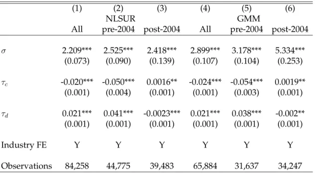
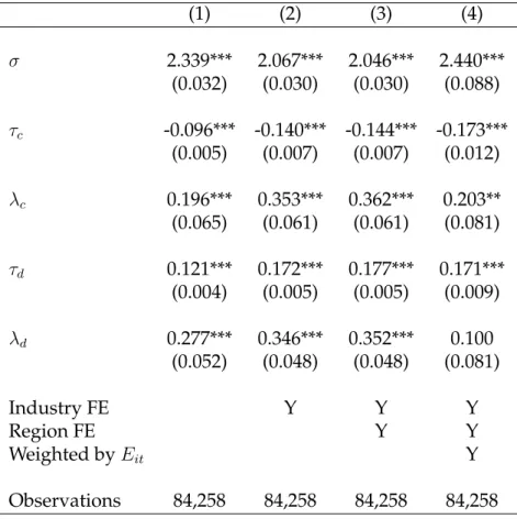
I try to investigate whether and to what extent such large-scale reforms in the energy sector affected the elasticity of substitution between clean and dirty energy and the bias in the direction of technological change. For the purpose, I re- estimate the system of equations (4) - (5) separately on the pre- (1994 - 2003) and post-intervention period (2004 - 2015). Table 7 reports the results. Column (1) repro- duces the estimation results from the baseline specification on the entire sample period with industry fixed effects (column (2) in Table 4) for reference. Results from the pre- and post-intervention period are reported in column (2) and (3), respectively. It is noteworthy that σis very similar across the two periods, remaining over 2 as in the main specification. In contrast, technical progress parameters change substan- tially: dirty-energy-biased technological change observed over the entire sample period appears to be largely driven by the trend in the pre-intervention period. In the post-intervention period, the estimated technological parameter associated with clean energy is now positive and precise, while that associated with dirty energy turns negative. Column (4)-(6) reports GMM estimates with the instruments. The σestimates tend to be much larger in the split samples. The technological progress parameters indicate the same pattern – a potential change in the direction of technological change that favors clean energy in recent years. However, estimation by sector reveals large heterogeneity across industries (Table A1). The technological

16Limited competition is due to the dominant role of the incumbent utility, for instance, Électricité de France (EDF) in the electricity market. EDF controls a large nuclear fleet with production costs lower than wholesale electricity prices.

17Marin and Vona (2017) explore in an econometric analysis the role of these energy policies in driving firm-level energy prices in France and find that the tax scheme applying to all final consumers of electricity (Contribution au Service Public de l’Electricité) had an impact of the largest magnitude, although the other two policies also had a significant impact on energy prices.

(18)

change is biased towards clean energy in the post-intervention period for 11 out of 19 industries.

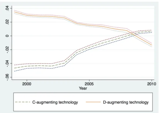
To check the possibility that the division of the sample period (before and after 2004) is arbitrary and the results depend on it, I estimate the system by GMM with the instruments on a 10-year rolling window and report the results from this exercise graphically in Figure 3. It is readily observable thatτ_c slowly reaches zero as the rolling window moves and starts including years after 2004 and eventually turns positive as the window safely moves into the post-intervention period. The opposite is observed forτ_d.

[Figure 3]

How do we reconcile these empirical observations with theory? One explana- tion is that the relative price of clean to dirty energy has been steadily decreasing, with the price of dirty energy increasing at a faster rate than the price of clean energy – clean energy was 3.5 times more expensive than dirty energy in 1994 but only 1.6 times more expensive in 2015. This decreasing price competitiveness of dirty fuels might have had a negative influence on the incentives to innovate dirty- energy-augmenting technology over time, although dirty energy was still cheaper than clean one in absolute levels.¹⁸

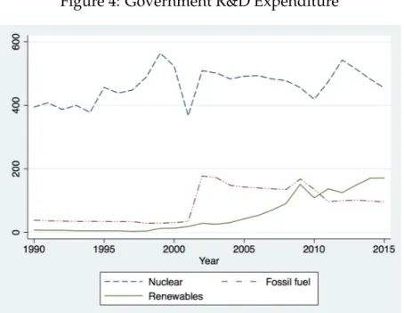
[Figure 4]

The literature has also emphasized the role of R&D subsidies for clean energy in inducing clean-energy-biased technological change (Acemoglu et al., 2012; Greaker et al., 2018; Hart, 2019). Figure 4 shows the government expenditure on R&D support for fossil fuels, renewables and nuclear over the period of 1994 - 2015 in France.

The data comes from the International Energy Agency (IEA). While subsidies for R&D related to nuclear remained highest with no clear pattern, government support for renewables grew continuously from early 2000, eventually exceeding support for fossil fuels around 2010.¹⁹ Although causal claims cannot be made, the increasing subsidies for clean energy appear to coincide with the technological progress biased towards clean energy observed from mid-2000 in the data.

18Indeed, in the presence of strong energy policies to move towards a low-carbon economy in France as well as in other countries, it is not realistic that firms would attempt to substitute away from clean to fossile-based energy in response to rising prices of clean energy despite the strong elasticity of substitution.

19This observation can be seen in the context of the comprehensive environmental programme launched in 2007,Grenelle de l’Environnement, which puts forward a series of policies and measures

(19)

4.4 Robustness checks

4.4.1 Alternative approaches

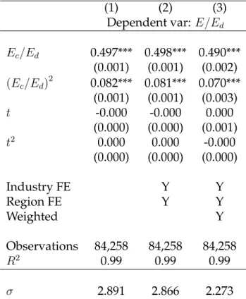
In this section, I test the sensitivity of the estimates to alternative specifications other than the system of equations approach by trying two other popular approaches used in the literature to estimate the elasticity of substitution, namely, the estimation of a linearized production function and of the FOCs. First, I try the Kmenta approximation, which is a first-order Taylor expansion of the CES function aroundσ = 1. The approximation leads to:

log E_it

E_it^d

=γ log E_it^c

E_it^d

+ (σ−1)γ(1−γ)

| 2σ{z }

a

log

E_it^c E_it^d

2

+ [γτ_c+ (1−γ)τ_d]

| {z }

b

t+ (σ−1)γ(1−γ)

2σ [τ_c−τ_d]²

| {z }

c

t² (7)

again assumingA^c_it = A^c₀e^τ^c^t, A^d_it = A^d₀e^τ^d^t andA^c₀ = A^d₀ = 1.²⁰ Usingˆγ, σis iden- tified from the compositea. One drawback of this specification is that it is difficult to identifyτ_c andτ_d without prior information on which technology parameter is larger. Thus, as in León-Ledesma et al. (2010), I use this specification to check for the robustness of theσestimates only. Results are reported in Table 8. Column (1) shows the estimate of σ around 2.9, which is comparable to those from the previous specifications. I include industry and region fixed effects in column (2). When weighted by the total energy consumption, the estimate falls but remains qualitatively similar to the previous ones.

[Table 8]

including specific plans for strengthening R&D on clean energy technologies in order to achieve France’s long-term greenhouse gas emissions reduction target (75 percent reduction by 2050) (IEA, 2009). For example, the government has provided subsidies through ae57 billion investment program “Investments for the Future” for the integration of renewable energy into industrial plants since 2010. The program includes full subsidies granted to research institutes, subsidies and grants to companies and direct capital investment for the development of renewable energy. Similarly, the government has initiated a series of calls for tenders since 2004 in order to stimulate investments in large-scale renewable energy plants (IEA, 2004, 2009).

20In approximation, the term that multiplies input ratio by the time trend, (σ−1)γ(1−γ) 2σ log ^E_E^it^cd

it t, is dropped as in León-Ledesma et al. (2010) without any significant loss of precision.

(20)

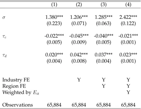
Second, I estimate the combined FOCs in equation (3), which I reproduce below, to estimate the elasticity of substitution and the overall bias in technological change (i.e.,τ_c−τ_d).

log E_it^d

E_it^c

=a₂+σ log P_it^c

P_it^d

+ (1−σ) (τ_c−τ_d)t+_it (8) In column (1) of Table 9, I find an OLS estimate of the elasticity of substitution between clean and dirty energy of 1.759, which is within the range of estimates from the system of equations approach reported above. Assuringly, the coefficient on the time trend is positive (0.048), which implies that the overall bias in technological change (τc−τ_d) is negative over the whole sample period (i.e., dirty-energy biased technological change) given the above-unity estimate of the the elasticity of substitution. When splitting the sample into pre- and post-2004, the implication re- garding the change in the direction of technological change is remarkably similar to the findings from the the system of equations approach: strongly dirty-energy biased technological change in the pre-2004 period and slightly clean-energy biased technological change in the post-2004 period (a positive and a negative coefficient on the time trend in column (2) and (3), respectively). Using the instruments developed in Section 4.2 yields similar results including the shift in the overall bias in technological change between pre- and post-2004 periods (column (4)-(6)). The similar estimates from alternative approaches reported in this section add confidence that the main estimates from the system of equations approach are not driven by the choice of the estimation method.

[Table 9]

4.4.2 Robustness of the system of equations approach

In this section, I check for the sensitivity of the system of equations approach by using alternative instruments for energy prices and alternative specifications for technological progress. I have so far used instruments that apply the growth rates of energy prices at the national level to the initial firm-level price, which effectively blocks the channel through which factor-specific technology at the firm level influences relative prices through the firm’s relative input demands. Other studies have implemented a similar specification that weights national fuel prices using the initial (thus fixed) fuel share at the firm level (Linn, 2008; Sato et al., 2019; Marin and

(21)

Vona, 2019). This specification mitigates the concern of endogenous change in fuel mix due to technological shocks at the firm level, which could lead to changes in relative input demands and prices.²¹ The alternative instrument for the price of clean energyP_it^c,IV is constructed as follows:

P_it^c,IV = X3

j=1

φ^j_i,t=t₀ P_t^j (9)

where P_t^j is the national price of fuel j and φ^j_i,t=t₁ is the initial share of fuel j in the clean energy bundle (that includes electricity, steam, and renewables) in the first year in which the firm appeared in the sample. The initial year is then dropped from the sample and therefore the sample period runs from 1995 rather than 1994 similarly as in Section 4.2. The alternative instrument for the price of dirty energyP_it^d,IV is similarly constructed with the initial share of each dirty fuel calculated within the dirty energy bundle.

Table 10 reports GMM estimates from using the alternative instruments. Theσ estimates tend to be smaller in magnitude than those in earlier specifications (except in column (4)), but remain above unity. Technology parameters across all columns suggest a largely dirty-energy-biased technological change. For instance, the clean- and dirty-energy-augmenting technology has experienced -2.1% and 2.3% per year growth, respectively (column (4)). To check the evolution of energy-specific efficiency growth over time, I estimate the system using the alternative instruments on a 10-year rolling window. The results are reported graphically in Figure 5. As before, one observes sharply different trends in the clean- and dirty-energy augmenting technology. Estimates of τ_c gradually increase over time turning positive as the window moves into the post-2004 period, while those ofτ_dgradually fall and turns negative around the same time.

[Table 10]

[Figure 5]

21This specification was not chosen as the preferred specification since changes in fuel mix are less worrisome in my context where energy is already partitioned into the clean and dirty bundle with the two most popular fuels, electricity and natural gas, belonging to each one. As a result, a change of the same magnitude in fuel mix is much less pronounced within the bundles than in the energy aggregate. Earlier studies that use this instrument (mentioned above) treat energy as a whole.

(22)

So far, I assumed linear constant technological progress, following the relevant empirical literature. As a robustness check, I try an alternative specification for technological progress that flexibly nests linear, log-linear and hyperbolic growth based on the Box-Cox transformation (Klump et al., 2007; León-Ledesma et al., 2010). This leads to the general expression, A_i(t) = e^gⁱ^(t) where g_i(t) = _λ^τⁱ

i

t^λⁱ−1

, i = c, d andt > 0. The curvature parameter λ_i determines the shape of the technological progress function. λ_i = 1implies the linear constant growth assumed so far;λ_i = 0 a log-linear specification; and λ_i < 0 a hyperbolic specification for technological growth. For instance, λ_c = 1 with τ_c > 0 and λ_d = 0 with τ_d > 0 corresponds to a scenario where the growth in clean-energy-augmenting technological progress is constant, while that in dirty-energy-augmenting technological progress continuously decelerates and asymptotically converges to zero.

Table 11 reports the estimates from this exercise. It is noteworthy that σ estimates remain comparable to those from the main specification despite the strong nonlinearities added by the new terms. The estimated technology parameters again suggest a largely dirty-energy-biased technological change over the sample period.

But, they are much larger in magnitude than those produced by the previous specifications and likely to be beyond what is economically reasonable: -14 % and 17%

per year growth in the clean- and dirty-energy-augmenting technology, respectively (column (3)), although both curvature parameters are below unity, implying that at least the growth in both technologies (or de-growth in the case of clean energy) decelerates and converges asymptotically to zero. León-Ledesma et al. (2010) also find that the bias in estimates from this specification tends to be higher compared to the linear specification for technological progress especially when σ is greater than 1. GMM estimates that account for potential endogeneity are also qualitatively similar (Table A2). Table A3 reports estimates from a 10-year rolling window to see how the rates of technological growth associated with each energy type evolve over time with this alternative specification for technological progress. Again, σ estimates remain above unity throughout. As observed in the previous specifications, the growth of clean-energy-augmenting technology appears to surpass that of dirty-energy-augmenting technology in the last two windows that sit squarely in the post 2004 period, and yet, again with economically unreasonable magnitudes of the estimates.

[Table 11]

(23)

5 Conclusion

The elasticity of substitution between clean and dirty energy and the direction of technological change, either dirty-energy-biased or clean-energy-biased, are central parameters in discussing one of the most challenging questions facing the world today, climate change. In most theoretical models that investigate the possibility of sustainable growth, the elasticity of substitution between clean and dirty energy plays a key role by determining the extent to which innovation efforts are encouraged towards the use of clean fuels, which ultimately allows sustainable growth.

However, there is limited consensus on the magnitude of this substitution elasticity and much less on the nature of technological change due to a dearth of empirical estimates for these key parameters. In this paper, I made an attempt to fill this gap in the literature by estimating the elasticity of substitution between clean and dirty energy inputs from micro data, jointly with technological parameters that capture the direction of technological change within the energy aggregate.

I find micro estimates of the elasticity of substitution between clean and dirty energy inputs greater than unity. The estimated technological progress parameters suggest the direction of technological change was largely biased towards dirty energy over the period of 1994 - 2015. The high estimated elasticity of substitution, coupled with the relative price movement with dirty energy being considerably cheaper than clean energy throughout the sample period, rationalizes the dirty-energy-biased technological change observed in the data. However, I also find evidence that government interventions had an impact on the direction of technological change – faster technological progress associated with clean energy with the changes in relative prices and higher subsidies for clean energy in recent years.

Although the findings presented in this paper provide a strong empirical foundation for a large number of papers that investigate the possibilities of sustainable growth with directed technological change, there is ample room for improvement and future research. For instance, expanding the method to include public and pri- vate R&D for improving overall energy efficiency and switching from traditional fossil-based fuels to cleaner fuels can shed light on causal links for the shift in the direction of technological change observed in the data. Furthermore, although the elasticity of substitution parameter is considered time-invariant, the kind of technological progress that allows substitution between factors easier, in other words,

‘sigma-augmenting’ technological change can be also very relevant, particularly in

(24)

the context of climate change. It has been noted in the macroeconomic literature that an increase in the elasticity of substitution between labor and capital has strong effects on growth, although the mechanisms are not well understood (Klump et al., 2012). I believe the knowledge of how such sigma-augmenting technological change may occur and operate will broaden the scope of our understanding of sustainable growth.

(25)

References

Acemoglu, D. (2002). Directed technical change. The Review of Economic Studies, 69(4):781–809.

Acemoglu, D., Aghion, P., Bursztyn, L., and Hemous, D. (2012). The environment and directed technical change. American Economic Review, 102(1):131–66.

Alexeeva-Talebi, V. (2011). Cost pass-through of the eu emissions allowances: Ex- amining the european petroleum markets. Energy Economics, 33:S75–S83.

Antras, P. (2004). Is the US aggregate production function Cobb-Douglas? New estimates of the elasticity of substitution. Contributions in Macroeconomics, 4(1).

Bartik, T. J. (1991). Who benefits from state and local economic development policies?

Borissov, K., Brausmann, A., and Bretschger, L. (2019). Carbon pricing, technology transition, and skill-based development. European Economic Review, 118:252–269.

Bretschger, L. (2015). Energy prices, growth, and the channels in between: Theory and evidence. Resource and Energy Economics, 39:29–52.

David, P. A. and Van de Klundert, T. (1965). Biased efficiency growth and capital- labor substitution in the US, 1899-1960. The American Economic Review, pages 357–

394.

Doraszelski, U. and Jaumandreu, J. (2018). Measuring the bias of technological change. Journal of Political Economy, 126(3):1027–1084.

Fabra, N. and Reguant, M. (2014). Pass-through of emissions costs in electricity markets. American Economic Review, 104(9):2872–99.

Fried, S. (2018). Climate policy and innovation: A quantitative macroeconomic analysis. American Economic Journal: Macroeconomics, 10(1):90–118.

Golosov, M., Hassler, J., Krusell, P., and Tsyvinski, A. (2014). Optimal taxes on fossil fuel in general equilibrium. Econometrica, 82(1):41–88.

(26)

Greaker, M., Heggedal, T.-R., and Rosendahl, K. E. (2018). Environmental policy and the direction of technical change. The Scandinavian Journal of Economics, 120(4):1100–1138.

Hansen, L. P. (1982). Large sample properties of generalized method of moments estimators. Econometrica: Journal of the Econometric Society, pages 1029–1054.

Hart, R. (2019). To everything there is a season: Carbon pricing, research subsidies, and the transition to fossil-free energy. Journal of the Association of Environmental and Resource Economists, 6(2):349–389.

Hassler, J., Krusell, P., and Olovsson, C. (2012). Energy-saving technical change.

Technical report, National Bureau of Economic Research.

IEA (2004). Energy Policies of IEA Countries: France 2009 Review.

IEA (2009). Energy Policies of IEA Countries: France 2009 Review.

Kalt, J. P. (1978). Technological change and factor substitution in the United States:

1929-1967. International Economic Review, pages 761–775.

Karydas, C. and Zhang, L. (2019). Green tax reform, endogenous innovation and the growth dividend. Journal of Environmental Economics and Management, 97:158–181.

Klump, R., McAdam, P., and Willman, A. (2007). Factor substitution and factor- augmenting technical progress in the United States: A normalized supply-side system approach. The Review of Economics and Statistics, 89(1):183–192.

Klump, R., McAdam, P., and Willman, A. (2012). The normalized CES production function: Theory and empirics. Journal of Economic Surveys, 26(5):769–799.

Lenzen, M. (2008). Life cycle energy and greenhouse gas emissions of nuclear energy: A review. Energy Conversion and Management, 49(8):2178–2199.

León-Ledesma, M. A., McAdam, P., and Willman, A. (2010). Identifying the elasticity of substitution with biased technical change. American Economic Review, 100(4):1330–57.

Linn, J. (2008). Energy prices and the adoption of energy-saving technology. The Economic Journal, 118(533):1986–2012.

(27)

Marin, G. and Vona, F. (2017). The impact of energy prices on employment and environmental performance: Evidence from french manufacturing establishments.

Technical report, SEEDS Working Paper 07/2017.

Marin, G. and Vona, F. (2019). Climate policies and skill-biased employment dy- namics: Evidence from eu countries. Journal of Environmental Economics and Man- agement, 98:102253.

Otto, V. M., Löschel, A., and Dellink, R. (2007). Energy biased technical change: A CGE analysis. Resource and Energy Economics, 29(2):137–158.

Panik, M. J. (1976). Factor learning and biased factor-efficiency growth in the United States, 1929-1966. International Economic Review, pages 733–739.

Papageorgiou, C., Saam, M., and Schulte, P. (2017). Substitution between clean and dirty energy inputs: A macroeconomic perspective.Review of Economics and Statis- tics, 99(2):281–290.

Raval, D. R. (2019). The micro elasticity of substitution and non-neutral technology.

The RAND Journal of Economics, 50(1):147–167.

Sato, M., Singer, G., Dussaux, D., and Lovo, S. (2019). International and sectoral variation in industrial energy prices 1995–2015. Energy Economics, 78:235–258.

Stern, D. I. (2012). Interfuel substitution: A meta-analysis. Journal of Economic Sur- veys, 26(2):307–331.

Wooldridge, J. M. (2010). Econometric analysis of cross section and panel data. MIT press.

(28)

Figures and Tables

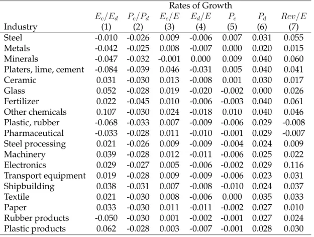
Table 1: Descriptive Statistics Rates of Growth

E_c/E_d P_c/P_d E_c/E E_d/E P_c P_d Rev/E

Industry (1) (2) (3) (4) (5) (6) (7)

Steel -0.010 -0.026 0.009 -0.006 0.007 0.031 0.055 Metals -0.042 -0.025 0.008 -0.007 0.000 0.020 0.015 Minerals -0.047 -0.032 -0.001 0.000 0.009 0.040 0.060 Platers, lime, cement -0.084 -0.039 0.046 -0.031 0.005 0.040 0.041 Ceramic 0.031 -0.030 0.013 -0.008 0.001 0.030 0.017 Glass 0.052 -0.028 0.019 -0.020 -0.002 0.000 0.026 Fertilizer 0.022 -0.045 0.010 -0.006 -0.003 0.040 0.061 Other chemicals 0.107 -0.030 0.024 -0.018 0.010 0.040 0.046 Plastic, rubber -0.068 -0.033 0.007 -0.009 -0.006 0.029 -0.008 Pharmaceutical -0.033 -0.028 0.011 -0.010 -0.001 0.029 -0.007 Steel processing 0.021 -0.026 0.009 -0.009 -0.004 0.024 0.009 Machinery 0.039 -0.028 0.012 -0.011 -0.006 0.025 0.022 Electronics 0.029 -0.027 0.005 -0.006 -0.002 0.029 0.116 Transport equipment 0.019 -0.028 0.009 -0.009 -0.006 0.023 0.031 Shipbuilding 0.038 -0.031 0.007 -0.008 -0.010 0.024 0.037 Textile 0.021 -0.030 0.008 -0.006 0.000 0.035 0.033 Paper 0.033 -0.030 0.011 -0.011 -0.002 0.027 0.010 Rubber products -0.050 -0.030 0.001 -0.002 -0.001 0.027 0.024 Plastic products 0.062 -0.028 0.003 -0.007 -0.001 0.028 0.030 Notes: Calculated for 1994-2015.

Table 2: Dispersion in the Share of Clean Energy Statistics 25th Median 75th

75/25 Ratio 1.98 2.65 3.10 90/10 Ratio 3.44 5.29 6.55 Source: EACEI, 1994-2015.

(29)

Figure 1: Share of Clean Energy for the Cement Industry

Source: Enquête sur les Consommations d’Énergie dans l’Industrie (EACEI), 1994-2015 .

Table 3: Correlation between energy efficiency and clean energy share

(1) (2) (3)

Energy efficiency 0.342*** 0.368*** 0.195***

(0.057) (0.059) (0.040)

Age -0.000* -0.000**

(0.000) (0.000)

N 86611 80481 80481